A Hybrid Framework for High-Performance Modeling of Three-Dimensional Pipe Networks

Abstract

Three-dimensional (3D) pipe network modeling plays an essential part in high performance-based smart city applications. Given that massive 3D pipe networks tend to be difficult to manage and to visualize, we propose in this study a hybrid framework for high-performance modeling of a 3D pipe network, including pipe network data model and high-performance modeling. The pipe network data model is devoted to three-dimensional pipe network construction based on network topology and building information models (BIMs). According to the topological relationships of the pipe point pipelines, the pipe network is decomposed into multiple pipe segment units. The high-performance modeling of 3D pipe network contains a spatial 3D model, the instantiation, adaptive rendering, and combination parallel computing. Spatial 3D model (S3M) is proposed for spatial data transmission, exchange, and visualization of massive and multi-source 3D spatial data. The combination parallel computing framework with GPU and OpenMP was developed to reduce the processing time for pipe networks. The results of the experiments showed that the hybrid framework achieves a high efficiency and the hardware resource occupation is reduced.

1. Introduction

With the continuous development and advancement of geographic information systems (GIS), it has become challenging for traditional two-dimensional GIS to meet the needs of geospatial visualizations and analysis [1,2]. With the widespread application of GIS in society, the application of three-dimensional (3D) scenes in smart cities is becoming deeper and wider [3,4,5]. The traditional two-dimensional management model has been unable to meet the actual needs of the pipe network and pipe big data information analysis, expression, and application. The three-dimensional pipe network occupies a large part of the application scenarios. The performance-based city planning includes data management, data modeling, data analysis and data visualization. Due to the large-scale data size, wide range and various pipeline networks and pipelines, both on the ground and underground, and the spatial distribution is complex and varied, high-performance modeling of 3D pipe networks remains challenging. It is therefore essential to study the 3D pipe network construction and high-performance rendering.

Geodesign is proposed in order to visualize models for city planning [6,7]. With the development of Building Information Modeling (BIM), a three-dimensional model of construction project or facility’s physical and functional characteristics, and a shared knowledge has gradually become a common data expression in the field of architecture. Resources provide a decision-making basis for the management of the life cycle of a project or a facility. At different stages of the life cycle, various stakeholders modify information through BIM to coordinate operations. BIM data is an important data source for 3D GIS [8,9]; it enables 3D GIS to move from macro to micro, and at the same time to achieve refined management—especially for pipe networks.

Utility networks are modeled using graph-theory abstractions [10,11], because the structure properties of graph provide network nodes and links. Most utility networks are based on two dimensional modeling design [12], but in some cases, applications such utility networks operate in 3D [13,14,15]. Pipe network is one type of utility network, the construction of a 3D pipe network is based on network science and GIS. As the BIM-oriented network model can be used in indoor network applications [16], a 3D pipe network should be used in both outdoor and indoor GIS. It is challenging to design 3D pipe networks by considering visualization, checking topology, data management, and 3D network analysis.

The 3D pipe network includes the pipe point portion and the pipeline portion. In the existing three-dimensional systems, the pipeline portion is normally constructed by vector line lofting, and the pipe point is generally built by manual modeling and then imported into the scene. The workflow of these pipe point models requires a lot of manpower and material resources. At the same time, for 3D pipe network data, the user’s data source is often vector point and line data. If the model’s display mode is adopted, data redundancy and extra workload are unfortunately inevitable. The maintenance of vector seed of point, line data and pipe point models is required as well. In addition, in some enterprise-level scenarios, pipe network data in 3D city models is extremely dense, and thus rendering these dense pipe networks requires a lot of hardware resources. Therefore, improving the carrying capacity and rendering performance of massive pipe network data can be the answer to current capacity and rendering performance limits.

GIS-based methods and modeling are widely used in urban planning [17,18,19,20,21]. GIS and BIM are located in two different sectors for building a smart city. BIM provides the data foundation, and GIS provides a spatial reference, spatial analysis and decision making [22,23,24]. The combination of BIM and GIS contributes to urban planning, water conservancy projects, railway information modeling, underground pipe network information modeling, ancient building modeling and other fields [25,26]. The integration of GIS and Computer-aided design (CAD) supplies new data sources for building a smart city [27,28]. A hybrid system for expanding 2D GIS into the 3D scene is an effective way to consider the integration of 2D GIS and 3D GIS [29]. There are fewer studies that focus on the integration of spatial data modeling for GIS, BIM, CAD, and oblique photography. It is critical to study the integration model for spatial 3D data.

The computing-intensive framework plays an essential part in high-performance based smart city applications [30]. Parallel computing is an effective way to visualize 3D city models [31,32]. 3D city modeling requires effective algorithms [33,34]. NVIDIA, inventor of the graphics processing unit (GPU), proposes a parallel computing framework based on computing unified device architecture (CUDA), which can be used to speed up the processing efficiency of geospatial applications [35,36,37]. The multi-threaded parallel processing based on multi-core central processing unit(CPU)s provides extensive computational capabilities [38,39]. The scientific computing for building city modeling is shifting from a CPU-centric central processing model to a collaborative processing model in which CPUs and GPUs work together [40].

In this paper, we propose a hybrid framework for high-performance modeling of 3D pipe networks. This paper is organized as follows: Section 2 introduces a pipe network data model, Section 3 shows hybrid high-performance modeling of 3D pipe networks, Section 4 describes the experiments and the results, and the last section is the conclusion and further work.

2. Pipe Network Data Model

The network data model is an essential part of high-performance modeling of 3D pipe networks.

2.1. Pipe Network Data Structure

A variety of pipe networks are normally represented hierarchically [41]. A network data set is used to describe a type of pipe network information. The data volume is less redundant and contains topology information, which can be used for subsequent spatial network analysis, such as burst analysis and connectivity analysis. Each pipeline data set consists of two sub-datasets: lines and nodes. The line sub-dataset represents pipeline objects, and the node sub-dataset represents point objects, such as elbows, tees, crosses, and valves.

Table 1. The pipe line structure in the network data set.

ID Number	From Node	To Node	PrePoint	NextPoint	Geometry Information
1	3	2	$(Y_{p_1},Y_{p_2})$	$(Y_{p_{n1}},Y_{p_{n2}})$	$(x_1,y_1,z_1)(x_2,y_2,z_2)\dots (x_n,y_n,z_n)$

shows the main structure of the attribute table of the line sub-dataset, where the ID field is the ID of the line object itself, the FromNode and ToNode fields record the ID of the node object connected to both ends of a line object, and the PrevPoint and NextPoint fields recording the geometric coordinates of the other endpoints of the other line objects connected at both ends can facilitate the subsequent construction of the visualized point model.$(x_i,y_i,z_i)$ is the i-th point coordinate of geometry information. In addition, the geometric coordinates of the line object itself and some attribute information are stored.

Table 2. The node structure in the network data set.

ID Number	Geometry Information
1	$(x_1,y_1,z_1)$
2	$(x_2,y_2,z_2)$
3	$(x_3,y_3,z_3)$
…	…
n	$(x_n,y_n,z_n)$

shows the main storage structure of the node sub-dataset, wherein the ID field is the ID of the pipe point object, the ID also corresponds to the FromNode and ToNode fields in the line sub-dataset, and a field for storing geometric information and attribute information. In these two associated data sets, the topology information is stored in the online data set.

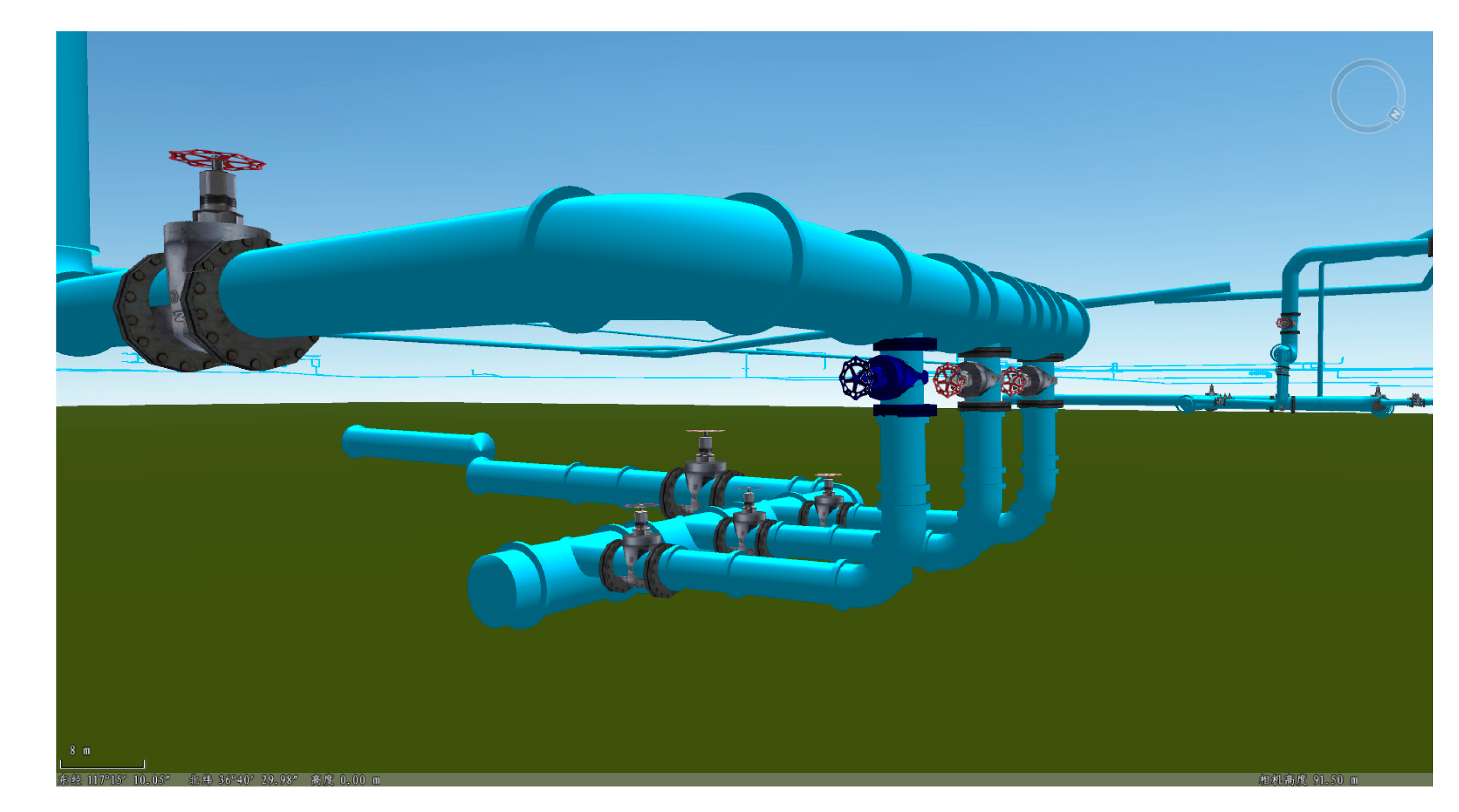
2.2. Construction of Pipeline Model

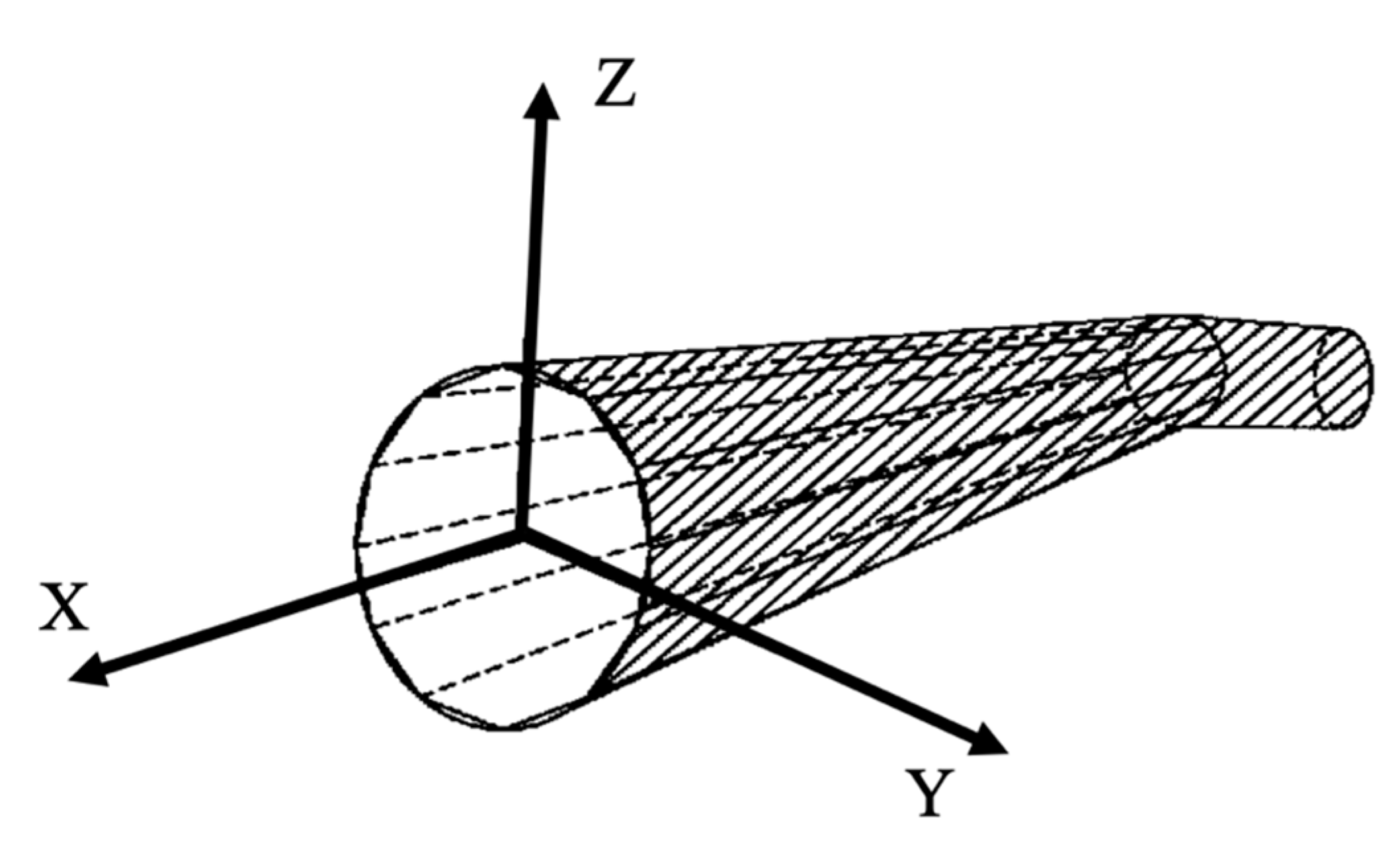
2.2.1. Coordinate Computation of Pipeline Network Model

After building the acquired pipeline data as a network dataset, it will be necessary to create a 3D pipeline network model for rendering. We use the pipe segment corresponding to the line segment between the two coordinates on the line geometry object of the pipeline as a rendering unit, and then combine these pipe segments to form the entire pipeline.

Each pipe segment consists of two sections, and if the position of the vertices on the two sections on the pipe section can be determined, an entire pipeline can be determined. We take the center of each section as the origin, the X-axis along the pipeline, and the Cartesian coordinate system on the Y-axis in the section (as shown in Figure 1). Since the cross-sectional shape of the pipeline is known, the position of the point on the pipe cross section in the local coordinate system can be determined. The position $P_s$ of the center of the section in the world coordinate system is stored in the geometric information of the online object so that the translation matrix ($M_t$) of the center of the section can be obtained.

To make the section perpendicular to the pipeline, and to make the upper direction of the pipeline section coincide with the upper direction in the world space, a rotation is also required. It is known that the world coordinate pointing to the center point of a given section is $W_1$, and the coordinate pointing to the center point of the next section along the strike direction is $W_2$, and the direction of the strike is ${\overrightarrow{V}}_{\sec }=W_1-W_2$, corresponding to the X-axis in the local coordinate system of the section, and the upper direction in the world space is ${\overrightarrow{V}}_{up}=(0,0,1)$, corresponding to the Z axis in the local coordinate system and the Y axis being ${\overrightarrow{V}}_r={\overrightarrow{V}}_{\sec }\times {\overrightarrow{V}}_{up}$, the rotation matrix $M_{rot}$ can be obtained. The coordinates of the final section vertices in the world coordinate system are defined as formulation (1).

$$P_w=M_{rot}·M_t·P_s.$$

(1)

It is worth noting that for a longitudinal tube, the up direction is the same or opposite to the direction. In this case, V_r calculated from the previous section can be used as the V_r of the current section, or any direction perpendicular to the direction can be specified as V_r.

2.2.2. Smoothing of Pipeline Inflection Points

When the pipeline is an inflection point, it is necessary to process the cross-section rotation matrix of the connected pipe segments before and after the inflection point so that the front and rear sections can be connected. The inflection point smoothing effect can be achieved by inserting several sections with smooth transitions, while the original two sections need to be retracted a distance to meet the smooth section, as shown in Figure 2.

In this study, the following algorithm was used to calculate the cross-sectional matrix smoothed by the inflection point: Project the two lines that meet the inflection point into the plane where the two lines are located. Make a circle in the plane tangent to the two lines. As shown in Figure 3, the arc AB is the position of the center-line of the transition section. The more transition sections you take on this section, the smoother the inflection point. The length of the point A to the inflection point O is the length M of the pipeline section that needs to be retracted. By the constraint that the radius of the circle cannot be greater than the width W of the pipeline, we can get the value of M using formulation (2):

$$M=\tan \theta *W.$$

(2)

The vector OA is defined as ${\overrightarrow{L}}_1$ and OB is defined as vector ${\overrightarrow{L}}_2$. Then, the center coordinate $(x_c,y_c,z_c)$ can be obtained by the following method:

$${\overrightarrow{P}}_l={\overrightarrow{L}}_1\times {\overrightarrow{L}}_2,$$

(3)

$$\begin{array}{l}{k}_1={\widehat{P}}_l·\widehat{O}\\ k_2={\widehat{L}}_1·\widehat{A}\\ k_3={\widehat{L}}_2·\widehat{B}\end{array},$$

(4)

$$\begin{array}{l}D={\widehat{P}}_l.x*{\widehat{L}}_1.y*{\widehat{L}}_2.z+{\widehat{P}}_l.y*{\widehat{L}}_1.z*{\widehat{L}}_2.x+{\widehat{P}}_l.z*{\widehat{L}}_1.x*{\widehat{L}}_2.y\\ -{\widehat{P}}_l.z*{\widehat{L}}_1.y*{\widehat{L}}_2.x-{\widehat{P}}_l.y*{\widehat{L}}_1.x*{\widehat{L}}_2.z-{\widehat{P}}_l.x*{\widehat{L}}_1.z*{\widehat{L}}_2.y\end{array},$$

(5)

$$\begin{array}{l}{x}_c=(k_1*{\widehat{L}}_1.y*{\widehat{L}}_2.z+k_3*{\widehat{P}}_l.y*{\widehat{L}}_1.z+k_2*{\widehat{P}}_l.z*{\widehat{L}}_2.y\\ -k_3*{\widehat{P}}_l.z*{\widehat{L}}_1.y-k_2*{\widehat{P}}_l.y*{\widehat{L}}_2.z-k_1*{\widehat{L}}_1.z*{\widehat{L}}_2.y)/D\end{array},$$

(6)

$$\begin{array}{l}{y}_c=(k_2*{\widehat{P}}_l.x*{\widehat{L}}_2.z+k_1*{\widehat{L}}_1.z*{\widehat{L}}_2.x+k_3*{\widehat{P}}_l.z*{\widehat{L}}_1.x\\ -k_2*{\widehat{P}}_l.z*{\widehat{L}}_2.x-k_1*{\widehat{L}}_1.x*{\widehat{L}}_2.z-k_3*{\widehat{P}}_l.x*{\widehat{L}}_1.z)/D\end{array},$$

(7)

$$\begin{array}{l}{z}_c=(k_3*{\widehat{P}}_l.x*{\widehat{L}}_1.y+k_2*{\widehat{P}}_l.y*{\widehat{L}}_1.x+k_1*{\widehat{L}}_1.x*{\widehat{L}}_2.y\\ -k_1*{\widehat{L}}_1.y*{\widehat{L}}_2.x-k_3*{\widehat{P}}_l.y*{\widehat{L}}_1.x-k_2*{\widehat{P}}_l.x*{\widehat{L}}_2.y)/D\end{array}.$$

(8)

From the coordinates of the center of the circle, the position of the transition section inserted in the arc can be easily obtained, and then the translation and rotation matrix of the section of the transition section can be calculated by the previous method.

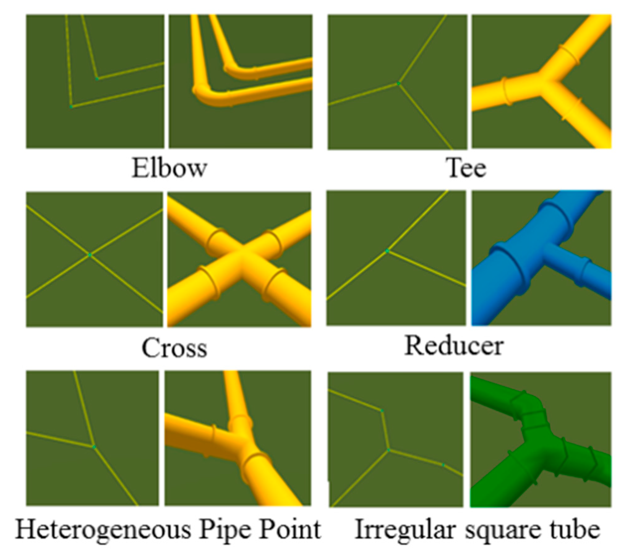
2.3. Construction of the Pipe Point Model

Pipe points such as elbows, tees, and crosses are essential parts of the pipeline scenario. In the previous pipeline information management systems, such a pipe point is normally constructed by a method manually and created in the modeling software, and then the modeled pipe point is imported into the scene. There are two main issues in the way of constructing the pipe point. The first is that the construction of the pipe point model is carried out in its own local coordinate system. Therefore, after the pipe point is imported into the scene, it is necessary to manually adjust its position direction so that the pipe points can be matched with the pipeline. The second is that due to the accuracy of the pipeline data collection, the angle between the pipe and the pipe point is different from the standard value. Therefore, the standard three-way and four-way models cannot be used to match the pipeline. It is necessary to construct a pipe point model for each angle, which greatly increases the workload of modeling.

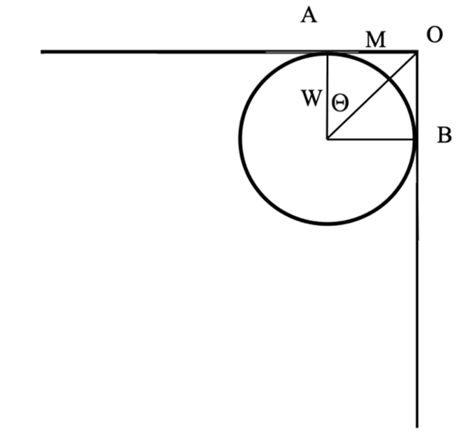
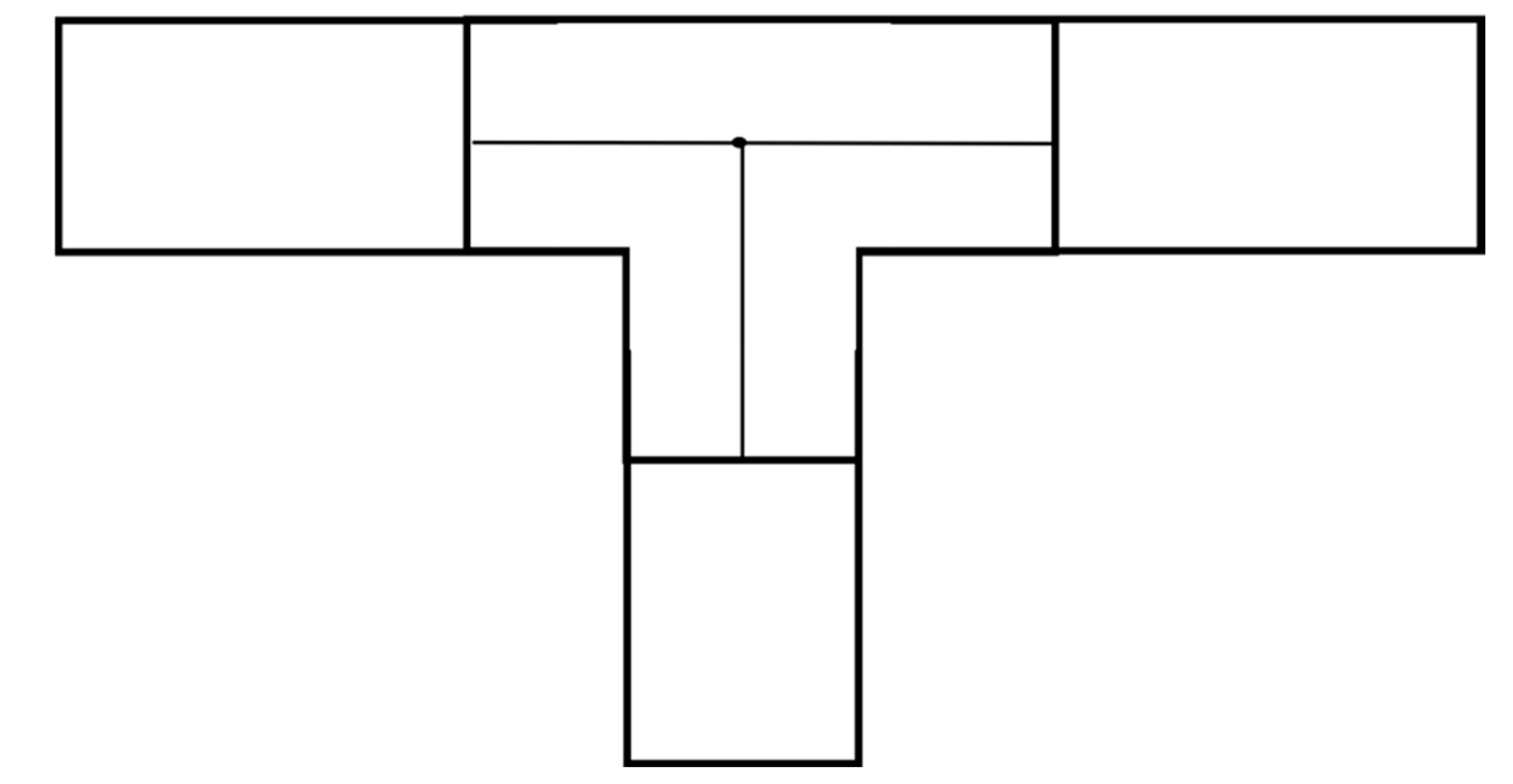
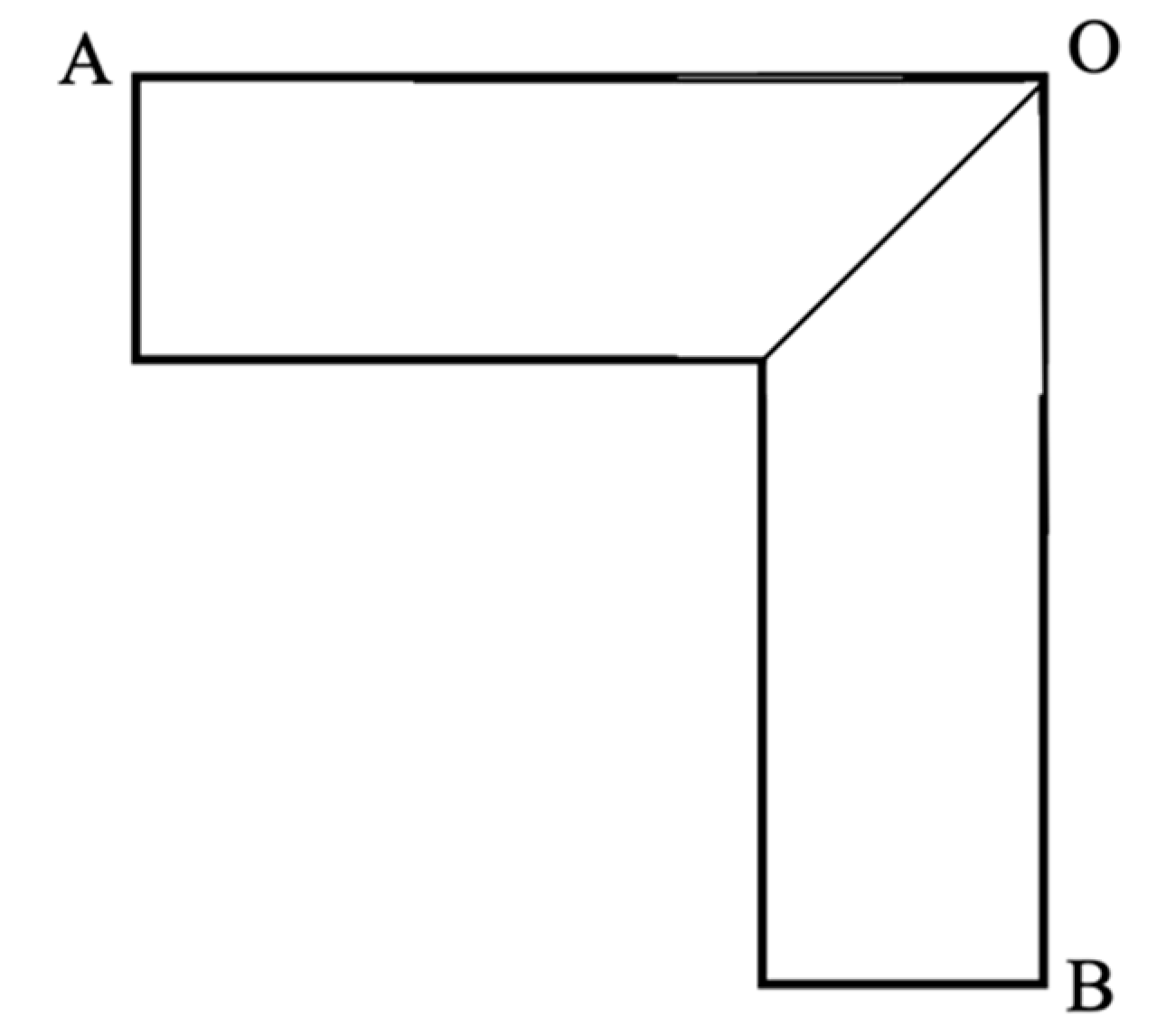
2.3.1. Constructing the Pipe Point Model

We propose a new method for constructing the pipe point model, which can quickly construct the elbows, tees, and crosses that match the connected pipelines. Among them, the elbow is a pipe point connected to two pipes. The following paragraph is an example of the construction of such a pipe point connected to two or more pipes by taking a multi-pass pipe point as an example.

A multi-pass point can be broken down into a combination of multiple half-pipe segments, as shown in Figure 4. The shape of each half pipe segment is determined by the center point of the pipe point and the direction of the pipe connected to it, so that one half-pipe segment becomes HalfPipePair. Its structure contains three points including first point (FirstPt), center point (CenterPt), and second point (SecondPt).

We define that the half pipe pair is made up of a section on the X > 0 side of the pipeline, and its direction is FirstPt->CenterPt->SecondPt.

Use the following algorithm to find the half pipe pairs needed to make up the multi-pass point.

(1)

Traverse the points A, B on each of the two pipelines, calculate their plane P with the center point O;

(2)

Traverse the other pipeline points C except for A and B, calculate the position it projects onto P, and record whether the half pipe pairs of $A\to O\to B$ and the half pipe pairs of $B\to O\to A$ are required as the boolean variables bneedAtoB and bneedBtoA. The initial value is true;

(3)

Determine the relationship between $C_p$ and $\angle AOB$. If $C_p$ falls inside $\angle AOB$, then bneedAtoB = false; if $C_p$ falls outside $\angle AOB$, then bneedBtoA = false;

(4)

After traversing the other points except for A and B, if the needAtoB is true, the half pipe pair $A\to O\to B$ is recorded. If the bneedBtoA is true, the half pipe pair $B\to O\to A$ is recorded; back to (1).

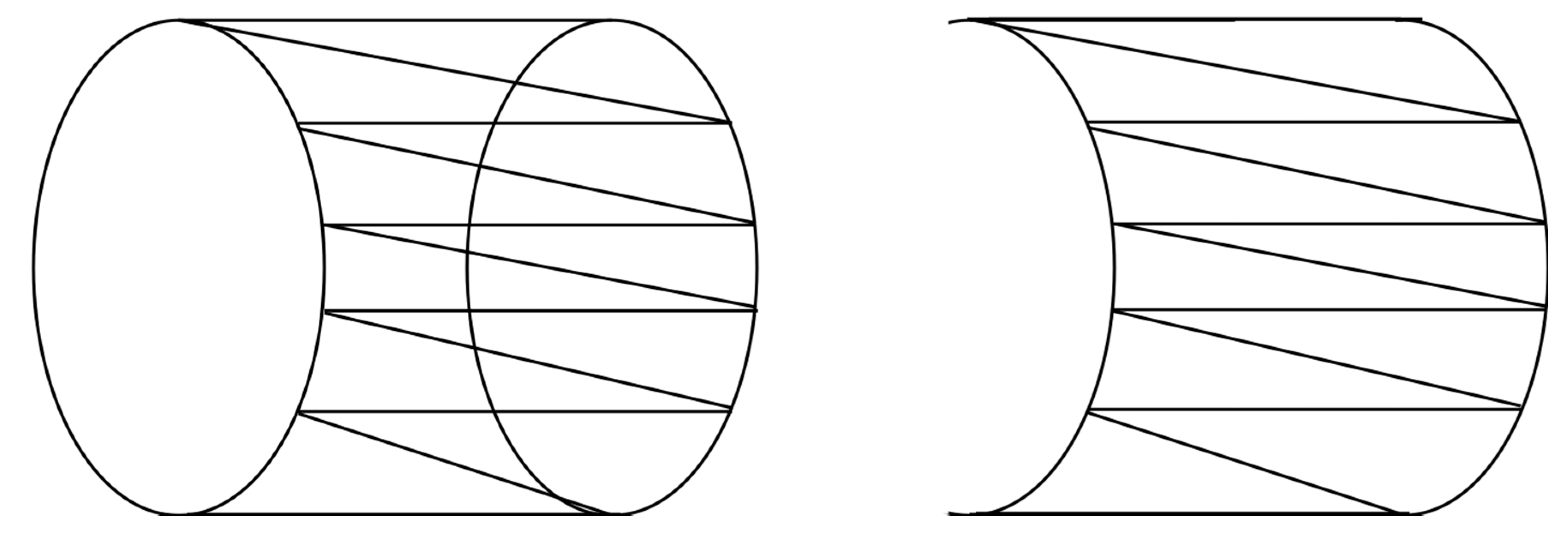
2.3.2. Matrix Computation of Half-Pipe

After a set of half-pipe pairs constituting the multi-pass pipe point are obtained, they need to be decomposed into pipe segment units. As shown in Figure 5, one half pipe pair can be broken down into two pipe segment units. The calculation of the section matrix that is connected to the pipeline is given in Section 2.2.1. The matrix calculation of the intersection of two pipe segments is described below. It is easy to know that the interface is the angle bisector of $\angle AOB$, and the trend is ${\overrightarrow{V}}_{\sec }=\overrightarrow{AO}+\overrightarrow{OB}$. Therefore, its rotation matrix can be calculated by the method in Section 2.2.1.

Let $\angle AOB$ be α, the normal vector of AOB plane be $\overrightarrow{P}$, and the angle between $\overrightarrow{P}$ and upper direction ${\overrightarrow{V}}_{up}$ be β. Then, the scaling ratios $Scal{e}_Y$ and $Scal{e}_Z$ of the Y and Z axes in the local coordinate system and the scaling matrix $M_{Scale}$ can be calculated. The vertex position on the half pipe segment is $P_W=M_{Scale}·M_{rot}·M_t·P_s$.

$$Scal{e}_Y=\sqrt{{\sin }^2\beta /{\sin }^2(\alpha *0.5)+{\cos }^2\beta },$$

(9)

$$Scal{e}_Z=\sqrt{{\cos }^2\beta /{\sin }^2(\alpha *0.5)+{\sin }^2\beta },$$

(10)

$$M_{Scale}=\left(\begin{array}{cccc}1& 0& 0& 0\\ 0& Scal{e}_Y& 0& 0\\ 0& 0& Scal{e}_Z& 0\\ 0& 0& 0& 1\end{array}\right).$$

(11)

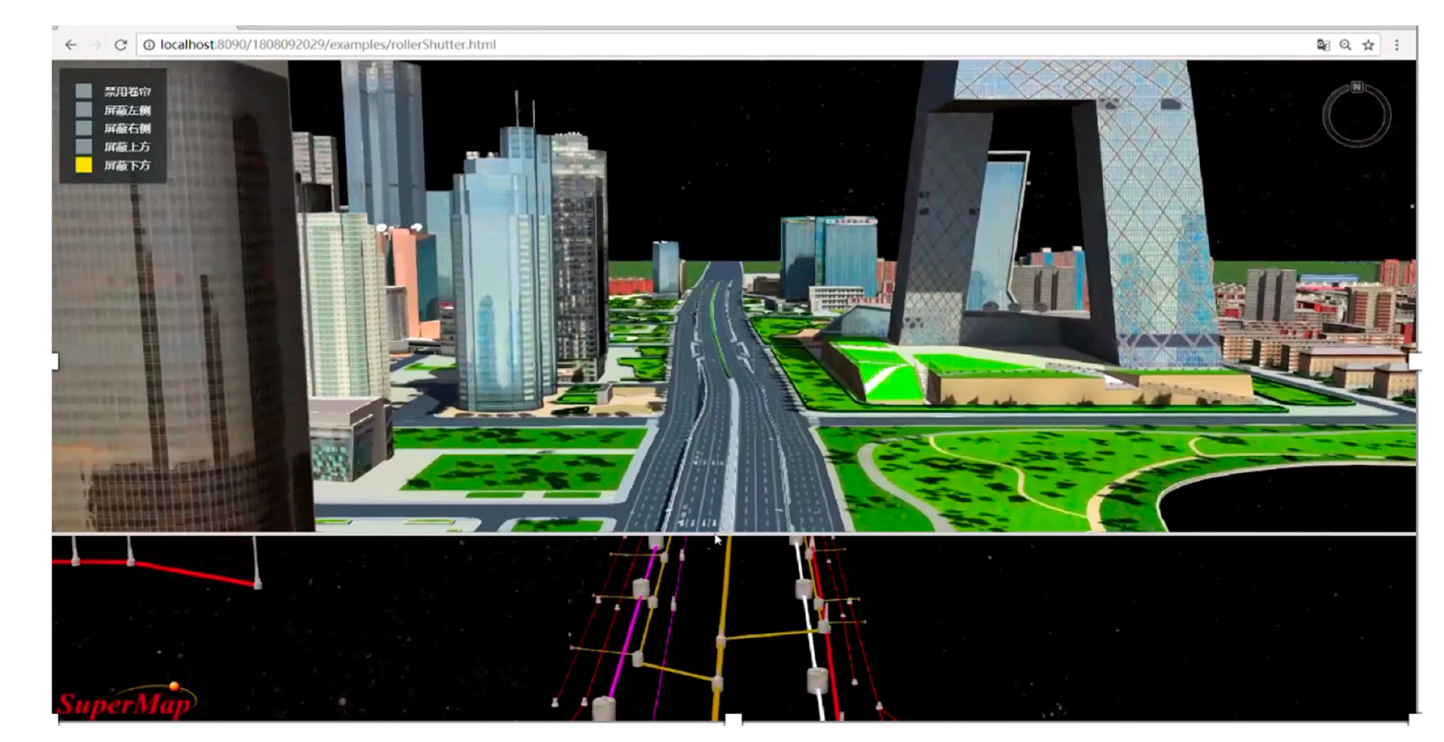
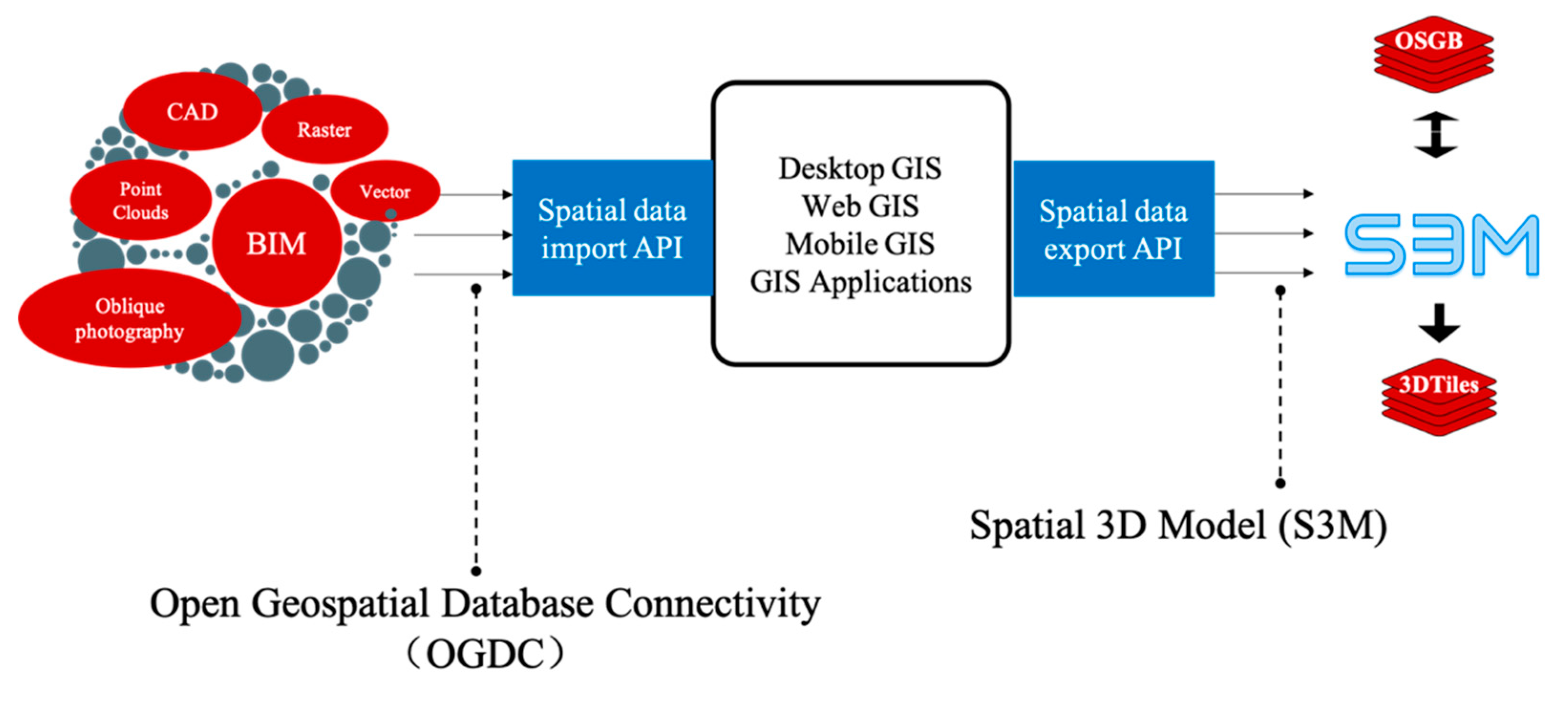
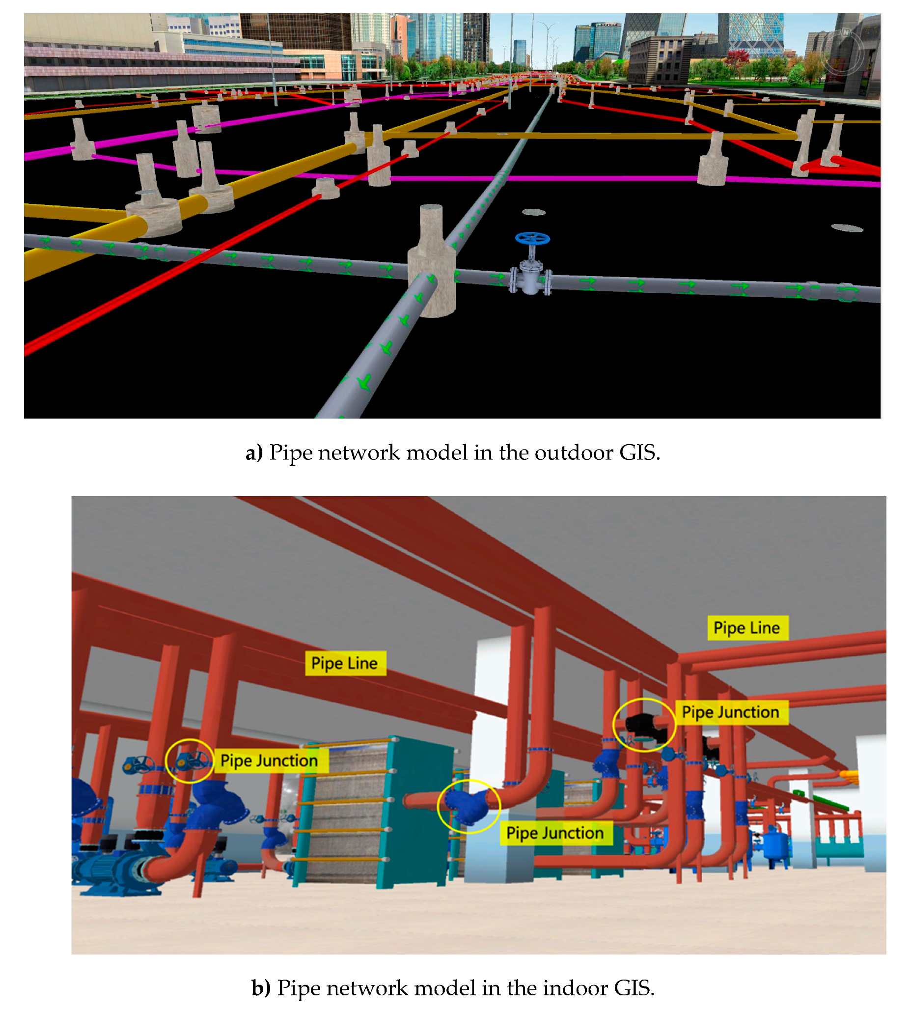
2.4. Integration Framework for 2D GIS and 3D GIS

The integration framework for 2D GIS and 3D GIS contains spatial data management integration, application integration, function module integration, expression symbol system integration, and analysis function integration. The essential part is that the spatial data model and spatial data structure of 2D and 3D data objects are kept in the same design. All the two-dimensional data can be directly used with high-performance modeling in the 3D scene without any spatial data conversion. 2D maps and 3D scenes can easily be generated based on the integration framework for 2D GIS and 3D GIS (Figure 6). The 2D and 3D integration of spatial data management solves the problem of spatial data compatibility of different dimensions and reduces the cost and complexity of the system construction to meet the needs of various applications. Spatial analysis is supported in both 2D map and 3D scene. 3D network analysis is widely used in pipeline network management. GPU graphics hardware acceleration provides a powerful support for 3D analysis functions and brings users a good experience with high performance.

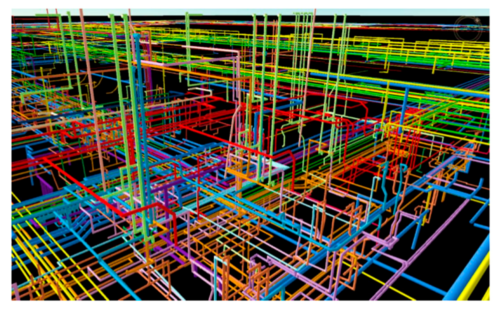
3. High-Performance Modeling for 3D Pipe Networks

The framework for high-performance modeling of 3D pipe network contains a spatial 3D model, instantiation, adaptive rendering, and combinational parallel computing.

3.1. Spatial 3D Model (S3M)

Spatial 3D model (S3M) is proposed for spatial data transmission, exchange and high-performance visualization of massive and multi-source 3D spatial data [42]. It meets the requirements of users in three-dimensional data transmission and analysis between different terminals (mobiles, browsers, and desktops) through an efficient and scalable data specification. S3M supports multi-source data, including pipelines, BIM, laser point clouds, vector, terrain, dynamic water surfaces, and 3D grids. S3M provides the ability to efficiently visualize a large amount of data using the level of details (LOD), batch rendering, and instantiation to improve the rendering performance.

The S3M includes description files, index tree files, data files, and attribute files. The file organization of each object storage is shown in

Table 3. The file organization of S3M.

Object	Storage Format	File Type	Description
TileTreeSetInfo	.scp	description file	description of the entire data
AttributeInfos	attribute .xml	attribute description file	description of each data set attribute in TileTreeSet
TileTree	Folder	data folder	store all data in the tile range
AttributeData	.xml	attribute data file	attribute data of all objects belong to the tile
IndexTree	.json	index tree file	all PagedLOD information belong to the tile
Tile	.s3mb	data file	a S3MB file stores data in a spatial division of the LOD layer

. S3M TileTreeSet object is the basic element in S3M. TileTreeSetInfo is its description information, which is an overall description of the data. If the TileTreeSet is constructed based on the point, line, polygon or model dataset, there may be an AttributeInfos that represents attribute description information for each data set. Space division of three-dimensional data are in a specified spatial range, each spatial division corresponding to a tree structure organization tile collection is represented by a TileTree object. IndexTree is index information of its tree structure. AttributeData representing attribute data are recorded in TileTree attribute data for each object. Each TileTree is subdivided step by step from top to bottom, and each space partition corresponds to one tile, represented by a Tile object.

The description file (.scp) and data folder are the basic components. The description file contains the path filename (.json) for each TileTree. The index file is a description of the tree structure of the tile data and can obtain the bounding box of the tile file of each layer, the switching information of the LOD and the attached child node file without loading the actual data. The main role is to accelerate the efficiency of tile file retrieval; the attribute data includes one attribute description file (attribute.xml) and a .xml file storing each tile attribute data in each TileTree. All tiles in TileTree form a tree-like logical structure.

To facilitate sharing of multi-source heterogeneous geospatial data, the open geospatial database connectivity (OGDC) was proposed to connect different types of geospatial data (Figure 7). OGDC provides a unified entry to geospatial data [43]. The unified data specifications, such as I3S [18] and S3M, can be used for high-performance, consistent access to data in the system, such as various GIS terminal applications, and user APPs.

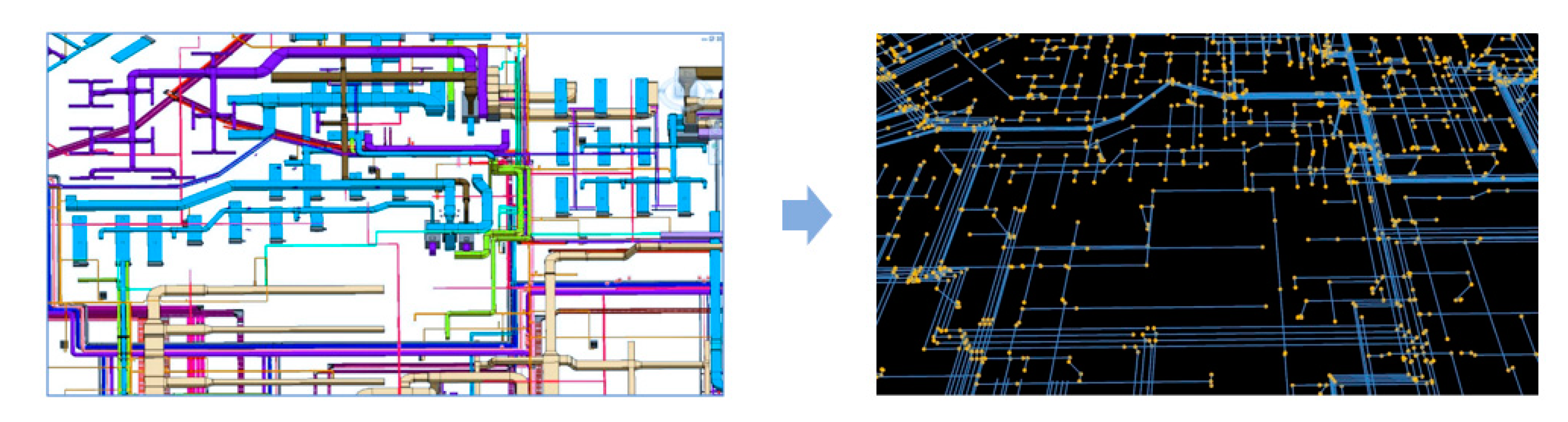
3.2. Instantiation Rendering of Pipe Networks

Instantiated rendering refers to multiple renderings of a grid using different parameters at different locations. Instantiation is often applied to the rendering of static mesh objects such as leaves, grass, etc. in a large number of scenes. All instances share a vertex buffer, which is used to store a single grid of data that will be instantiated multiple times. The instance buffer is used to store instance data for each object, including the information such as transformation matrices, color data, and lighting data. The rendering process is combined with a vertex buffer and an instance buffer for rendering.

The pipeline is in fact composed of pipe sections that are substantially similar and have slightly different positions and directions. In order to render these slightly different pipe segments, the traditional method is to store each pipe segment separately, which consumes a lot of memory resources; or it needs to switch frequently between rendering states, such as rotating and panning each pipe segment, which significantly affects rendering performance. By instantiating the grid of reused pipe segments, reducing the number of calls and memory requirements, and giving most of the rendering work to the GPU, reducing the CPU load is a good way to improve rendering performance.

For the instantiation of the pipe point pipeline, only two sets of grids need to be established. One set is a complete section pipe section for rendering the elbows in the pipeline and the pipe points, and the other set is a half-section pipe section for rendering the multi-pass pipe points. As shown in Figure 8, the different tube segment examples differ in the position of the cross-section at both ends, in the size of the zoom, and in the direction. These can be represented by two transformation matrices M_Bottom and M_Top. The matrix stores 18 floating point numbers representing the three rows and three columns of the two matrices into the instance buffer, and the grid data of the pipe segment is stored in the vertex buffer. In addition, the vertex needs to be stored in the vertex attribute of the vertex buffer, to which the matrix belongs before and after. Finally, the vertex position of the pipeline can be calculated by multiplying the vertices of the static mesh with the matrix in the vertex shader.

3.3. Adaptive Rendering for Pipe Network Data

The BIM data structure includes a spatial data model and attributes data. The spatial data model includes spatial information and appearance shape. The attribute data includes design parameters, construction parameters and operation, and maintenance parameters. The 3D GIS covers the data structure of BIM (spatial data and attribute data), covering the data representation of BIM (3D model), covering BIM data objects (BIM for architectural objects, and GIS covers a wide range, including architectural objects), and it overlaps with the BIM function (information management and spatial analysis). The 3D underground pipeline scene based on BIM-GIS consists of three-dimensional pipe points and three-dimensional pipelines. The three-dimensional pipeline includes round pipes, square grooves, pipe blocks, and vertical pipes. Three-dimensional pipe points include three types of feature points, wells and ancillary facilities: feature points such as elbows, straight throughs, three-way, cover plugs, and pipe caps. Wells include square wells, round wells, and rain rafts. Ancillary facilities include valves and water meters. Based on the BIM technology, this study uses linear symbols to construct three-dimensional pipelines and adaptive pipe point symbols to construct three-dimensional pipe points. Some special feature points, wells, and ancillary facilities are displayed by model symbols.

BIM model symbols can be used to visualize the pipe points with complex shapes, such as valves. However, in the three-dimensional scene, the model symbols cannot adaptively adjust the angle according to the direction of the pipeline in the X, Y, and Z directions. Due to the influence of the model angle, the pipe point deviates from the scene, for example, the pipe at the bottom of the valve cannot be connected with the pipeline and the valve switch is covered by a pipe. We can convert the BIM model to 3D pipe network using S3M (Figure 9).

An adaptive rendering model is proposed with the combinations of the data structure of the BIM model and the spatial structure characteristics of 3D GIS. The adaptive rendering model contains a pipe layer setting method and a symbol matching method. The pipe point layer was shown in a custom thematic map, specifying a property field as the symbol style of the thematic map. After setting the parameters of the symbol model, the symbol matching method adjusts the angle according to the pipeline orientation, including the pipe at the bottom of the valve in the pipeline direction, and the valve switch perpendicular to the pipeline direction (Figure 10).

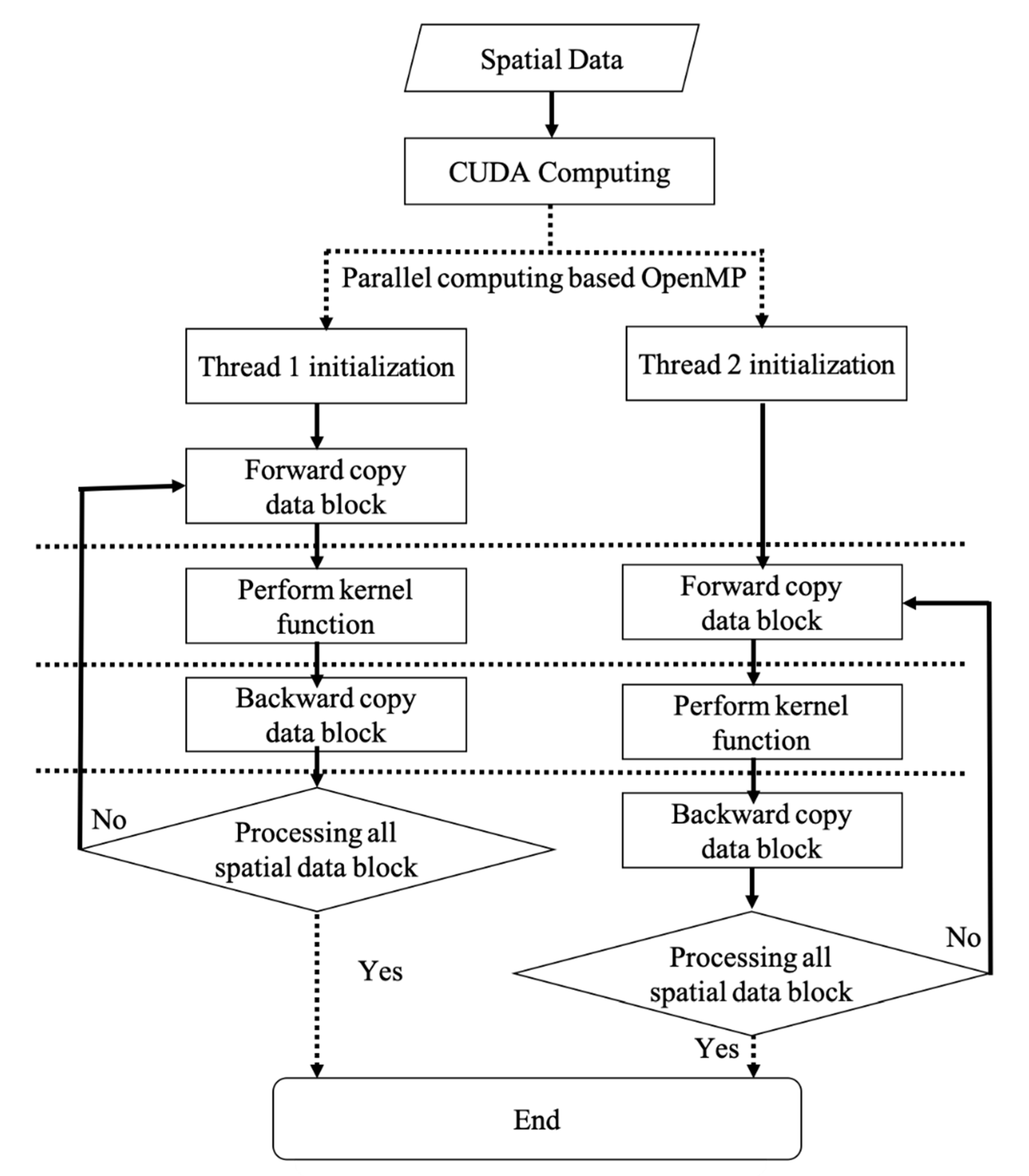
3.4. Combination Computing Framework with GPU and OpenMP

Rendering large-scale 3D pipe networks requires intensive computational time. The combinational parallel computing framework with GPU and OpenMP can greatly improve computing intensive pipe network-based applications. Considering that the spatial data exchange between the memory and the memory is time-consuming, and the large pipe network data cannot be copied to video memory at one time. We used the method of reading the pipe network data into the video memory. At the same time, we introduce the multi-thread processing strategy based on OpenMP to minimize the time occupation of GPU computing and data exchange to achieve the purpose of hiding data exchange time as much as possible.

Each CUDA core is only responsible for calculating the pixel result value of one specific location at the same time, and the kernel function specifies the specific calculation method. The specific workflow of a kernel function is to obtain the location of the pixel according to the built-in thread ID, and obtain the neighboring pixel at the location of the pixel (Figure 11). Then, the cell value is calculated based on the specific operator. Among them, the temporary variable corresponding to the neighboring pixel value is stored by using the shared memory inside the CUDA thread block, which can effectively improve the analysis performance. The computational resources were recycled when the combinational parallel computing framework was finished.

4. Experiments

The 3D pipe network model was implemented and the performance of the visualization is verified. The open source GIS projects are developed to verify the efficiency for the hybrid method of modeling the 3D pipe network. 3D pipe network model can be shown in desktop GIS, mobile GIS, and web GIS. The iDesktop-cross [44] is an open source desktop GIS project [45], which includes 3D pipe network models. The SuperMap iClient GIS (iClient-JavaScript [46]) is a visual analytics framework for WebGIS based application [7]. The pipe network data is shown in the outdoor GIS (Figure 12a) and the indoor GIS (Figure 12b).

Based on the API provided by iClient3D for WebGL [47], the pipe network visualization is shown in Figure 13 and is developed by SuperMap iEarth for WebGL [48].

To test the performance using the methods above, we use the instantiation and non-instantiation techniques to test the performance of the applications of 3D pipeline networks. The experimental environment is in the 64-bit Windows 7 operating system with 4 GB memory, the graphics card uses GTX650 with 2 G memory, and the CPU is an Intel i5-3340 with 3.1 GHz quad-core processor. The test scenario is pipeline data of a certain plant area, the area is about 5 km², and the pipeline is densely distributed, as shown in Figure 14. We specify the flight route in the scene, then let the camera automatically move along the flight path, recording the frame rate, CPU usage, and memory usage at each moment along the way.

The experimental results are shown in

Table 4. The result of benchmark experiment.

Experiment Type	Rendering Frame Rate	Percentage of CPU (%)	Physical Memory (MB)	Video Memory (MB)
Non-instantiation method	32.44	32.29	580.39	340-550
Instantiation method	61.66	9.34	552.57	310-360

. By using the instantiation method, the frame rate is increased by about 100%, the CPU usage is reduced to 33%, the memory usage is reduced to 25%, and the memory usage is slightly reduced. Proving that instantiation technology improves pipeline rendering performance is significant.

5. Conclusions and Discussion

In summary, we propose a hybrid framework for high-performance modeling of 3D pipe network, including pipe network data model and high-performance modeling. The pipe network is decomposed into two sections described in Section 2, and the multi-pass pipe point is decomposed into a set of pipe segments described by two half sections, through the topological relationship between the pipe point and the pipeline. Through this decomposition, complex pipe points can be split into simple units. In this way, a well-matched pipe point pipeline model can be quickly constructed, saving a lot of manual operations and improving the efficiency of building pipeline scenarios. In addition, the split pipe segment unit can be easily combined with the instantiation technique for rendering.

The results of the experiments have shown that the use of instantiation technology significantly improves the rendering performance of the 3D pipe networks. 3D pipe network design needs more time. The hybrid method reduces the cost for constructing 3D pipe network scene and improves the rendering performance of 3D pipelines and 3D pipe points. The geospatial application of 3D pipe network is complex. Spatial 3D model (S3M) is proposed for spatial data transmission, exchange, and visualization of massive and multi-source 3D spatial data. Rendering large-scale 3D pipe networks requires intensive computational resources. The combination parallel computing framework with GPU and OpenMP significantly reduces the processing time for large-scale 3D pipe networks. The results of the experiments showed that the hybrid framework achieves a high efficiency and the hardware resource occupation is reduced.

The hybrid framework for high-performance modeling of 3D pipe network that integrates geospatial applications makes GIS integrate into the high-performance based smart city with unprecedented opportunities. There are however some limitations to this study. (1) This study did not consider spatial cloud computing and edge computing, which is more powerful than hybrid parallel computing. Spatial cloud computing can address the high-performance based challenges for large-scale geospatial applications because spatial cloud computing has the ability to process large-scale 3D GIS models with high performance. Edge computing enables spatial analytics and geospatial data gathering to process near the source of the spatial data. Edge computing has the opportunity to perform real-time 3D pipe network modeling. (2) Our models did not consider artificial intelligence (AI) properties. 3D pipe network data production takes a long time with manual work. It is essential to extract the pipe network data from LiDAR data and remote sensing images using AI-based methods. In future work, we will focus on the integration of spatial cloud computing, edge computing, and machine learning to high-performance based smart city applications.

References

1. Zhong, E. Geocontrol and live geography: Some thoughts on the direction of gis. J. Geo-Inf. Sci. 2013, 15, 783–792. [Google Scholar]
2. Anejionu, O.; Thakuriahab, P.; McHugh, A.; Sun, Y.; McArthur, D.; Mason, P.; Walpol, R. Spatial urban data system: A cloud-enabled big data infrastructure for social and economic urban analytics. Future Gener. Comput. Syst. 2019, 98, 18. [Google Scholar] [CrossRef]
3. Biljecki, F.; Ledoux, H.; Stoter, J. An improved lod specification for 3D building models. Comput. Environ. Urban Syst. 2016, 59, 25–37. [Google Scholar] [CrossRef]
4. Wang, S.; Zhong, Y.; Wang, E. An integrated gis platform architecture for spatiotemporal big data. Future Gener. Comput. Syst. 2019, 94, 160–172. [Google Scholar] [CrossRef]
5. Yu, M.; Yang, C. A 3D multi-threshold, region-growing algorithm for identifying dust storm features from model simulations. Int. J. Geogr. Inf. Sci. 2017, 31, 939–961. [Google Scholar] [CrossRef]
6. Wu, C.-L.; Chiang, Y.-C. A geodesign framework procedure for developing flood resilient city. Habitat Int. 2018, 75, 78–89. [Google Scholar] [CrossRef]
7. Wang, S.; Zhong, E.; Cai, W.; Zhou, Q.; Lu, H.; Gu, Y.; Yun, W.; Hu, Z.; Long, L. A visual analytics framework for big spatiotemporal data. In Proceedings of the 2nd ACM SIGSPATIAL Workshop on Analytics for Local Events and News, Seattle, WA, USA, 6 November 2018; ACM: New York, NY, USA; p. 3. [Google Scholar]
8. Borrmann, A.; Kolbe, T.H.; Donaubauer, A.; Steuer, H.; Jubierre, J.R.; Flurl, M. Multi-scale geometric-semantic modeling of shield tunnels for gis and bim applications. Comput. Aided Civ. Infrastruct. Eng. 2015, 30, 263–281. [Google Scholar] [CrossRef]
9. Amirebrahimi, S.; Rajabifard, A.; Mendis, P.; Ngo, T. A framework for a microscale flood damage assessment and visualization for a building using bim–gis integration. Int. J. Digit. Earth 2016, 9, 363–386. [Google Scholar] [CrossRef]
10. Bakalov, P.; Hoel, E.G.; Kim, S. A network model for the utility domain. In Proceedings of the 25th ACM SIGSPATIAL International Conference on Advances in Geographic Information Systems, Redondo Beach, CA, USA, 7–10 November 2017; ACM: New York, NY, USA; p. 32. [Google Scholar]
11. Oliver, D.; Hoel, E.G. A trace framework for analyzing utility networks: A summary of results (industrial paper). In Proceedings of the 26th ACM SIGSPATIAL International Conference on Advances in Geographic Information Systems, Seattle, WA, USA, 6–9 November 2018; ACM: New York, NY, USA; pp. 249–258. [Google Scholar]
12. Alam, S.N.; Haas, Z.J. Coverage and connectivity in three-dimensional underwater sensor networks. Wirel. Commun. Mob. Comput. 2008, 8, 995–1009. [Google Scholar] [CrossRef]
13. Hijazi, I.; Ehlers, M.; Zlatanova, S.; Isikdag, U. Ifc to citygml transformation framework for geo-analysis: A water utility network case. In Proceedings of the 4th International Workshop on 3D Geo-Information, Ghent, Belgium, 4–5 November 2009. [Google Scholar]
14. Hijazi, I.; Ehlers, M.; Zlatanova, S.; Becker, T.; van Berlo, L. Initial investigations for modeling interior utilities within 3d geo context: Transforming ifc-interior utility to citygml/utilitynetworkade. In Advances in 3D Geo-Information Sciences; Springer: Berlin/Heidelberg, Germany, 2011; pp. 95–113. [Google Scholar]
15. Becker, T.; Nagel, C.; Kolbe, T.H. Integrated 3d modeling of multi-utility networks and their interdependencies for critical infrastructure analysis. In Advances in 3D Geo-Information Sciences; Springer: Berlin/Heidelberg, Germany, 2011; pp. 1–20. [Google Scholar]
16. Teo, T.-A.; Cho, K.-H. Bim-oriented indoor network model for indoor and outdoor combined route planning. Adv. Eng. Inform. 2016, 30, 268–282. [Google Scholar] [CrossRef]
17. Li, X.; Yeh, A.G.-O. Modelling sustainable urban development by the integration of constrained cellular automata and gis. Int. J. Geogr. Inf. Sci. 2000, 14, 131–152. [Google Scholar] [CrossRef]
18. Su, D.Z. Gis-based urban modelling: Practices, problems, and prospects. Int. J. Geogr. Inf. Sci. 1998, 12, 651–671. [Google Scholar] [CrossRef] [PubMed]
19. Moghadam, S.T.; Toniolo, J.; Mutani, G.; Lombardi, P. A gis-statistical approach for assessing built environment energy use at urban scale. Sustain. Cities Soc. 2018, 37, 70–84. [Google Scholar] [CrossRef]
20. Zhang, X.; Ma, G.; Jiang, L.; Zhang, X.; Liu, Y.; Wang, Y.; Zhao, C. Analysis of spatial characteristics of digital signage in beijing with multi-source data. ISPRS Int. J. Geo-Inf. 2019, 8, 207. [Google Scholar] [CrossRef]
21. Liu, K.; Gao, S.; Lu, F. Identifying spatial interaction patterns of vehicle movements on urban road networks by topic modelling. Comput. Environ. Urban Syst. 2019, 74, 50–61. [Google Scholar] [CrossRef]
22. Song, Y.; Wang, X.; Tan, Y.; Wu, P.; Sutrisna, M.; Cheng, J.; Hampson, K. Trends and opportunities of bim-gis integration in the architecture, engineering and construction industry: A review from a spatio-temporal statistical perspective. ISPRS Int. J. Geo-Inf. 2017, 6, 397. [Google Scholar] [CrossRef]
23. Zhu, J.; Wright, G.; Wang, J.; Wang, X. A critical review of the integration of geographic information system and building information modelling at the data level. ISPRS Int. J. Geo-Inf. 2018, 7, 66. [Google Scholar] [CrossRef]
24. Kang, T.W.; Hong, C.H. A study on software architecture for effective bim/gis-based facility management data integration. Autom. Constr. 2015, 54, 25–38. [Google Scholar] [CrossRef]
25. Liu, X.; Wang, X.; Wright, G.; Cheng, J.; Li, X.; Liu, R. A state-of-the-art review on the integration of building information modeling (bim) and geographic information system (gis). ISPRS Int. J. Geo-Inf. 2017, 6, 53. [Google Scholar] [CrossRef]
26. Karan, E.P.; Irizarry, J.; Haymaker, J. Bim and gis integration and interoperability based on semantic web technology. J. Comput. Civ. Eng. 2015, 30, 04015043. [Google Scholar] [CrossRef]
27. Bansal, V. Integrated cad and gis–based framework to support construction planning: Case study. J. Archit. Eng. 2017, 23, 05017005. [Google Scholar] [CrossRef]
28. Quan, S.J.; Li, Q.; Augenbroe, G.; Brown, J.; Yang, P.P.-J. Urban data and building energy modeling: A gis-based urban building energy modeling system using the urban-epc engine. In Planning Support Systems and Smart Cities; Springer: Berlin/Heidelberg, Germany, 2015; pp. 447–469. [Google Scholar]
29. Yu, L.-J.; Sun, D.-F.; Peng, Z.-R.; Zhang, J. A hybrid system of expanding 2D gis into 3D space. Cartogr. Geogr. Inf. Sci. 2012, 39, 140–153. [Google Scholar] [CrossRef]
30. Hu, M.; Li, C. Design smart city based on 3S, internet of things, grid computing and cloud computing technology. In Internet of Things; Springer: Berlin/Heidelberg, Germany, 2012; pp. 466–472. [Google Scholar]
31. Biljecki, F.; Stoter, J.; Ledoux, H.; Zlatanova, S.; Çöltekin, A. Applications of 3d city models: State of the art review. ISPRS Int. J. Geo-Inf. 2015, 4, 2842–2889. [Google Scholar] [CrossRef]
32. Liang, J.; Gong, J.; Zhou, J.; Ibrahim, A.N.; Li, M. An open-source 3D solar radiation model integrated with a 3D geographic information system. Environ. Model. Softw. 2015, 64, 94–101. [Google Scholar] [CrossRef]
33. Luo, F.; Zhong, E.; Cheng, J.; Huang, Y. Vgis-collide: An effective collision detection algorithm for multiple objects in virtual geographic information system. Int. J. Digit. Earth 2011, 4, 65–77. [Google Scholar] [CrossRef]
34. Luo, F.; Zhong, E.; Cao, G.; Tellez, R.D.; Gao, P. Vgis-antijitter: An effective framework for solving jitter problems in virtual geographic information systems. Int. J. Digit. Earth 2013, 6, 28–50. [Google Scholar] [CrossRef]
35. Ortega, L.; Rueda, A. Parallel drainage network computation on cuda. Comput. Geosci. 2010, 36, 171–178. [Google Scholar] [CrossRef]
36. Wu, J.; Deng, L.; Paul, A. 3d terrain real-time rendering method based on cuda-opengl interoperability. IETE Tech. Rev. 2015, 32, 471–478. [Google Scholar] [CrossRef]
37. Zhang, J.; You, S. Cudagis: Report on the design and realization of a massive data parallel gis on gpus. In Proceedings of the 3rd ACM SIGSPATIAL International Workshop on GeoStreaming, Redondo Beach, CA, USA, 6 November 2012; ACM: New York, NY, USA; pp. 101–108. [Google Scholar]
38. Zhou, C.; Chen, Z.; Pian, Y.; Xiao, N.; Li, M. A parallel scheme for large-scale polygon rasterization on cuda-enabled gpus. Trans. GIS 2017, 21, 608–631. [Google Scholar] [CrossRef]
39. Zhang, X.; Huang, C.; Min, G.; Wu, Y.; Zuo, Y. Distributed machine learning in big data era for smart city. In From Internet of Things to Smart Cities; Chapman and Hall/CRC: Boca Raton, FL, USA, 2017; pp. 151–177. [Google Scholar]
40. Heitzler, M.; Lam, J.C.; Hackl, J.; Adey, B.T.; Hurni, L. Gpu-accelerated rendering methods to visually analyze large-scale disaster simulation data. J. Geovis. Spat. Anal. 2017, 1, 3. [Google Scholar] [CrossRef]
41. Perelman, L.S.; Allen, M.; Preis, A.; Iqbal, M.; Whittle, A.J. Multi-level automated sub-zoning of water distribution systems. In Proceedings of the 7th Intl. Congress on Env. Modelling and Software, San Diego, CA, USA, 15–19 June 2014. [Google Scholar]
42. SuperMap. Spatial 3d Model Project. Available online: https://github.com/SuperMap/s3m-spec (accessed on 20 July 2019).
43. SuperMap. The Open Geospatial Database Connectivity Project. Available online: https://github.com/SuperMap/OGDC (accessed on 20 July 2019).
44. SuperMap. The Idesktop-Cross Project. Available online: https://supermap-idesktop.github.io/SuperMap-iDesktop-Cross/ (accessed on 20 July 2019).
45. Cai, W.; Wang, S.; Zhong, E.; Hu, C.; Liu, X. Design and implementation of a new cross-platform open source gis desktop software. Bull. Surv. Mapp. 2017, 1, 122–125. [Google Scholar]
46. SuperMap. The Iclient-Javascript Project. Available online: https://github.com/SuperMap/iClient-JavaScript (accessed on 20 July 2019).
47. SuperMap. The Iclient3d for Webgl Project. Available online: https://enonline.supermap.com/SuperMap_iClient3D_9.0.1_for_WebGL/ (accessed on 20 July 2019).
48. SuperMap. Supermap Iearth for Webgl Project. Available online: http://www.supermapol.com/earth/ (accessed on 20 July 2019).
Figure 1. Local coordinate system of pipe section.
Ijgi 08 00441 g001
Figure 2. Construction of smooth tube.
Ijgi 08 00441 g002
Figure 3. The result of the inflection point projected onto the plane.
Ijgi 08 00441 g003
Figure 4. The division of multi-way pipe.
Ijgi 08 00441 g004
Figure 5. The plane projection of half tube.
Ijgi 08 00441 g005
Figure 6. Pipe network models in 2D GIS and 3D GIS.
Ijgi 08 00441 g006
Figure 7. The heterogeneous geospatial data fusion framework.
Ijgi 08 00441 g007
Figure 8. The grid of section and half cross section.
Ijgi 08 00441 g008
Figure 9. From BIM model to 3D pipe network data model.
Ijgi 08 00441 g009
Figure 10. The adaptive rendering map in 3D GIS.
Ijgi 08 00441 g010
Figure 11. The workflow of the combinational parallel computing framework with GPU and OpenMP.
Ijgi 08 00441 g011
Figure 12. Pipeline network model in iDesktop Cross.
Ijgi 08 00441 g012
Figure 13. Pipeline network in the SuperMap iEarth.
Ijgi 08 00441 g013
Figure 14. Pipeline network in the experiment.
Ijgi 08 00441 g014