Abstract
Quickly and efficiently monitoring soil nutrient contents using remote sensing technology is of great significance for farmland soil productivity, food security and sustainable agricultural development. Current research has been conducted to estimate and map soil nutrient contents in large areas using hyper-spectral techniques, however, it is difficult to obtain accurate estimates. In order to improve the estimation accuracy of soil nutrient contents, we introduced a GA-BPNN method, which combined a back propagation neural network (BPNN) with the genetic algorithm optimization (GA). This study was conducted in Guangdong, China, based on soil nutrient contents and hyperspectral data. The prediction accuracies from a partial least squares regression (PLSR), BPNN and GA-BPNN were compared using field observations. The results showed that (1) Among three methods, the GA-BPNN provided the most accurate estimates of soil total nitrogen (TN), total phosphorus (TP) and total potassium (TK) contents; (2) Compared with the BPNN models, the GA-BPNN models significantly improved the estimation accuracies of the soil nutrient contents by decreasing the relative root mean square error (RRMSE) values by 15.9%, 5.6% and 20.2% at the sample point level, and 20.1%, 16.5% and 47.1% at the regional scale for TN, TP and TK, respectively. This indicated that by optimizing the parameters of BPNN, the GA-BPNN provided greater potential to improving the estimation; and (3) Soil TK content could be more accurately mapped by the GA-BPNN method using HuanJing-1A Hyperspectral Imager (HJ-1A HSI) (manufacturer: China Aerospace Science and Technology Corporation; Beijing, China) data with a RRMSE value of 20.37% than the soil TN and TP with the RRMSE values of 40.41% and 34.71%, respectively. This implied that the GA-BPNN model provided the potential to map the soil TK content for the large area. The research results provided an important reference for high-accuracy prediction of soil nutrient contents.
1. Introduction
Soil is an important component of terrestrial ecosystems and provides necessary moisture and nutrients for plant growth. As a main source of plant nutrition and soil, nutrients such as nitrogen, phosphorus and potassium play a vital role in plant growth [1,2]. Although traditional measurement methods (including field and laboratory measurements) provide accurate estimates of soil nutrient contents at sampled points, they are time-consuming and costly for the generation of spatially explicit estimates for a whole study area. For example, in China the analysis cost of every soil sample to obtain the contents of total nitrogen (TN), total phosphorus (TP) and total potassium (TK) in a laboratory is about ¥165 ($24). If a 100 m × 100 m spatial resolution map for an area of 50 km × 50 km is produced using the traditional methods, the total cost of obtaining the spatially explicit estimates of the soil properties for the whole area will be ¥2965 million ($424 million). This cost also ignores the traveling cost, and the time and labor for collection of soil samples in the field. Thus, traditional measurement methods do not meet the need of modern soil management. On the other hand, remote sensing technologies could quickly lead to spatially explicit estimates of soil nutrient contents and monitor their dynamics at regional scales with low cost [3]. This is mainly because remote sensing images provide spectral reflectance values on the basis of pixel-by-pixel with large coverages and repeated spectral measurements. Moreover, remote sensing-based methods focus on developing relationships of soil properties with spectral variables from images based on the field measurements from soil samples and then apply the relationships to estimate soil properties at the unobserved locations. Substantial research has been conducted in this field, especially for agricultural areas. For example, Dean et al. (2011) used airborne hyperspectral images to quantitatively estimate the 15 important soil elements (e.g., potassium, nitrogen, etc.) in tilled agricultural fields [4]. Gao et al. (2011) constructed the relationships between hyperspectral data and soil total nitrogen and organic matter contents using a high signal noise ratio measuring system to predict the contents of the soil properties in northeast China [5]. Xu et al. (2018) performed image pan-sharpening of Landsat 8 with WorldView-2 and Pleiades-1A using three pan-sharpening techniques, analyzed the relationships between pan-sharpened–multi-spectral indices and soil TN, and developed the soil TN prediction models using Random Forest methods in Bijarpur district, Karnataka State, South India [6].
Various studies using hyperspectral techniques to estimate soil nutrient contents have been reported. The present hyperspectral estimation methods of soil nutrient contents can be divided into two categories: linear and nonlinear predictions. The linear prediction methods build linear mathematical relationships between spectral variables from images and soil nutrient contents. Of them, the multiple linear regressions (MLR) and partial least squares regression (PLSR) are often used [7,8,9]. Due to their stability, the relationships often lead to an ideal estimation accuracy for specific research areas. However, they usually fail when the relationships are applied to other areas.
With the development of machine learning, many scholars have used nonlinear methods to estimate soil nutrient contents. The nonlinear methods mainly include various machine learning models to construct the nonlinear relationships between spectral variables and soil nutrient contents for prediction. The nonlinear models, including support vector machine (SVM), random forest (RF) and back-propagation neural network (BPNN), have been widely used to predict soil TN, TP, TK, organic matter and so on [10,11,12,13,14]. However, these models also have their own disadvantages. For example, SVM is difficult to implement for large-scale training samples because quadratic programming routines have high complexity and require huge memory and computational time for large area applications [15,16,17]. Random forests are prone to over fitting on regression models when RF models learn the detail and noise in training data that negatively impact the performance of the models on new data [18]. The BPNN algorithm has a strong nonlinear ability of modeling the relationships between soil nutrient contents and spectral variables from images, learning adaptability, and fault tolerance, which has been widely used to estimate contents of soil nutrients [19]. Substantial research [20,21,22,23,24] has also demonstrated that the BPNN method is a good alternative for this purpose. However, the large uncertainties of weights and threshold may affect the improvement of estimation accuracy for soil nutrient contents [25].
The objective of this study was to determine a method to accurately estimate soil nutrient contents for large areas using hyperspectral data by integrating the genetic algorithm (GA) with BPNN to optimize the weights and threshold of the network. The integration led to a new model GA-BPNN for the estimation of soil nutrient contents. The specific objectives were to: (1) use the GA-BPNN to construct a high-accuracy model to predict the contents of soil nutrients; and (2) apply the high-accuracy model to map the soil nutrient contents at a regional scale using HuanJing-1A Hyperspectral Imager (HJ-1A HSI) image. This method was examined to predict and map the contents of soil nutrients TN, TP and TK in a large area using hyperspectral data collected from the measurements of soil samples in laboratory and in a relatively small area using a HJ-1A HSI image, respectively.
2. Materials and Methods
2.1. Study Areas
This study dealt with both the whole Guangdong province and the Conghua district of Guangzhou in the province. Guangdong Province is one of the most developed areas in China with an area of 179,700 km2 and located in Southern China with the latitude and longitude ranges of 20°09′ to 25°31′ N and 109°45′ to 117°20′ E (Figure 1). The annual average temperature of the province is 21.8 °C and the annual average number of sunshine hours increases from less than 1500 h in the north to more than 2300 h in the south. The annual total solar radiation is between 4200 and 5400 MJ·m−2, and the annual average precipitation is 1789.3 mm. Lateritic red soil, red soil and lateritic soil dominate this area. A total of 75 soil samples were collected throughout the province in May 2017 and used for developing the hyperspectral estimation models of the contents of soil nutrients (TN, TP, and TK) (Figure 1).
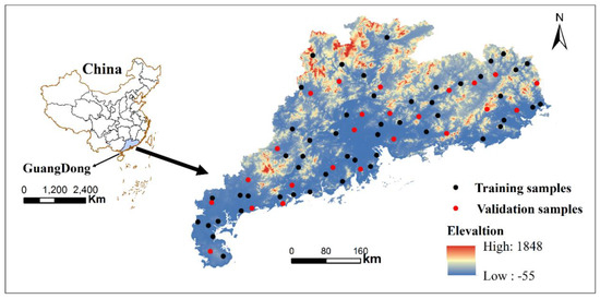
Figure 1.
The study area for model development with spatial distribution of soil samples.
In the Conghua district of Guangzhou city (Figure 2a), a total of 33 soil samples (red points in Figure 2b) were collected on 30 October 2017 and used for the accuracy validation of the model applications at the regional scale. In order to validate the application of the established models to hyperspectral satellite data, an HJ-1A HIS image at the 100 m spatial resolution and the view width of 50 km were selected to accurately and timely monitor the soil nutrient contents and map their spatial distributions because it has obvious advantages in regional macro-ecology remote sensing monitoring and evaluation [26]. The HJ-1A HSI image dated on 30 October 2017 was acquired with a total of 115 bands from 459 nm to 956 nm with a spectral resolution of 5 nm. Radiometric correction of the HJ-1A HIS image was conducted using fast line-of-sight atmospheric analysis of hypercubes (FLAASH) model. Geometric precision correction for the HJ-1A HSI data was conducted by using the quadratic polynomial calculation model and a cubic convolution interpolation method, and the geometric correction errors were controlled within 0.5 pixels.
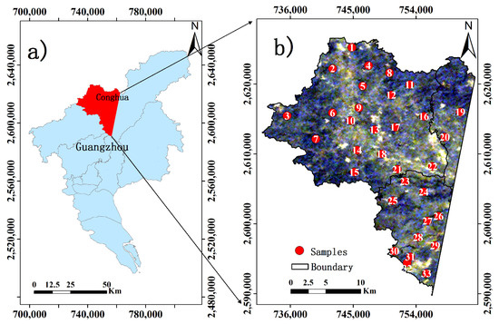
Figure 2.
(a) The location of the testing study area in Guangzhou city and (b) the area shown using the HJ-1A HSI image with the spatial distribution of the 33 test soil samples (red dots).
2.2. Soil Samples
2.2.1. Collection and Chemical Analysis of Soil Samples
In order to ensure the homogeneous distribution of the soil samples in Guangdong province, 75 soil samples were collected at a 50 km × 50 km sampling grid according to a stratified sampling method in this study (Figure 1). The 75 samples were randomly divided into 50 training samples (black dots in Figure 1) for model developments and 25 validation samples (red dots in Figure 1) for assessment of model predictions. Moreover, 33 soil samples (red dots in Figure 2b) in the Conghua district were employed to assess the accuracy of mapping soil nutrient contents at the regional scale using the HJ-1A HIS image. All the soil sample points were located using a global positioning system (GPS) receiver. At each sample point, five soil sub-samples of 0–20 cm depth soil layer were collected, mixed and used as the soil sample of this point. The soil samples were stripped of impurities, air dried, milled and filtered with a 2 mm sieve. The TN was measured using the semi-micro Kjeldahl method described by Walkley and Black [27]. The TP and TK were analyzed by ultraviolet spectrophotometer UV-2600 (made by Shimadzu CO, LTD.) and flame photometer FP640 (made by INESA Analytical Instrument CO, LTD.), respectively.
In order to enhance understanding of the data, descriptive statistics of the dataset from 75 soil samples were calculated in Table 1. The contents of soil TN, TP and TK ranged from 0.21 g kg−1 to 2.79 g kg−1, 0.13 g kg−1 to 3.75 g kg−1 and 0.62 g kg−1 to 30.39 g kg−1 with the mean values of 1.36 g kg−1, 0.75 g kg−1 and 10.55 g kg−1, respectively. The coefficients of variation (CV) of TN, TP and TK were 41.91%, 73.33% and 72.13%, respectively. The variability of the soil nutrient contents in the study area was moderate for TN and great for TP and TK [8], indicating that the 75 soil samples were reasonable. In addition, the sample means were not significantly different from each other between the training and test datasets at the significant level of 0.05.

Table 1.
Descriptive statistics of soil nutrient contents from 75 soil samples in Guangdong, China (TN: total nitrogen; TP: total phosphorus; TK: total potassium; St. Dev: standard deviation; CV: coefficient of variation).
2.2.2. Spectral Measurement and Pre-Treatment of Soil Samples
The spectral reflectance values of soil samples were measured with an AvaField portable spectrometer (Avantes, Inc., Holland) with a high signal-to-noise ratio (SNR) and high reliability (http://www.avantes.cn), which has a wavelength range of 340–2511 nm and a spectral sampling interval of 0.6 nm. The experiment was carried out in a black box, and each of the soil samples was placed in a black paper cup having a diameter of 10 cm and a depth of 7 cm. A 50 W (650 lx) halogen lamp was used to simulate sunlight with a 10° field of view (FOV). The soil spectral reflectance values were measured by vertical contact with the soil sample, and the white plate was used for calibration before the data collection to obtain the absolute reflectance. In order to improve the accuracy of measured soil reflectance, spectral sampling was performed in the center location of four zoning within the scope of soil samples. For each of the four sensing locations, 5 spectra were recorded, and the mean value of the 20 spectra was used to represent the soil spectral value at that point. In order to reduce the noise introduced in the process of spectral measurement, the spectra were smoothed using the piecewise Savitzky-Golay (SG) filter with a window size of 10 [28,29], and the smoothed curves of spectral reflectance for the soil samples are shown in Figure 3.
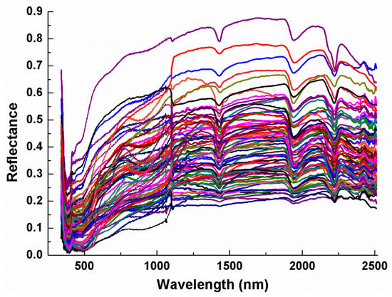
Figure 3.
Spectrum curves of 75 soil samples.
Figure 3 illustrates the spectral absorption features of the reflectance curves for each of the 75 soil samples. The characteristics of the waveform and absorption peak of these spectral curves are consistent with the current research [30,31,32], indicating that the collected soil spectral data are of high quality.
The differences in the spectral response of each soil nutrient can be so subtle that it is difficult to detect them using raw spectral data. In order to improve the prediction accuracy, the smoothed spectral data of soil nutrients were transformed with the First Derivative (FD), Second Derivative (SD) and Reciprocal Logarithmic (RL), which attempted to eliminate or reduce the effect of background noise and the change of signal intensity caused by the soil surface spectral scattering and absorption. The results are shown in Figure 4.
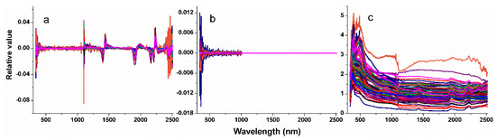
Figure 4.
Transformed spectral indices of soil samples: (a) First derivative spectral curves; (b) Second derivative spectral curves; and (c) Reciprocal logarithmic spectral curves.
2.3. Modeling and Mapping Methods
2.3.1. Selection of Spectral Variables
One of the most important steps for obtaining accurate hyperspectral estimation models of the soil TN, TP and TK contents was the determination of appropriate spectral variables. As an indication on the strength of the linear relationship between two random variables [20,33], Pearson correlation was used to select the spectral variables with the greatest correlation coefficients under the condition of significant level p ≤ 0.05. The Pearson correlation coefficient is expressed as:
where is the correlation coefficient between a soil nutrient content and a spectral variable, is the spectral reflectance of the i-th band of the nth soil sample, is the mean value of the reflectance of the soil sample in the i-th band, and is one of the soil nutrient (TN, TP and TK) contents, is the average value of a soil nutrient content.
In addition, the Variance Inflation Factor (VIF) was used to reduce the collinearity among the spectral variables. When 0 < VIF < 10, there was no collinearity relationship, when 10 ≤ VIF < 100, there was a strong collinearity relationship, and when VIF ≥ 100, there was a severe collinearity relationship [34,35].
2.3.2. Partial Least Squares Regression to Estimate Soil Nutrient Contents
The PLSR is a standard multivariate statistical technique that was developed by Herman Wold in 1966 [36]. The PLSR has been widely used in different disciplines because it allows for the analysis of data with strong correlations in the predictor variables, even when the number of training samples is far smaller than that of predictor variables [37]. The equation of PLSR is as follows:
where is the dependent variable (each of the soil nutrient contents) after mean centering; is the mean-centered independent variable matrix (spectral variables); is the coefficient matrix, and is the residual matrix.
2.3.3. Back-Propagation Neural Network to Estimate Soil Nutrient Contents
The BPNN is a multi-layer feed forward network trained by the error back propagation algorithm, which is suitable for various nonlinear relationship analysis. It consists of an input layer, an output layer and several hidden layers [38,39]. The trainlm and purelin were selected as the training function and the transfer function of the output layer in the BPNN. The steepest descent method and the back-propagation algorithm in the BPNN Model are used to repeatedly adjust the weight and deviation of the network until the actual value and the expected output are as close as possible [4,40], whose structure is shown in Figure 5a.
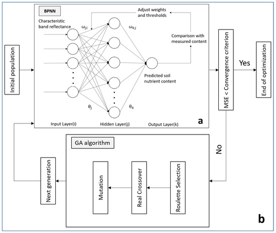
Figure 5.
The structures of (a) back propagation neural network (BPNN) and (b) GA-BPNN.
The BPNN network training includes two stages: forward propagation and error back propagation [41].
(1) Forward propagation
In neural networks, the forward propagation needs to calculate the neuron’s input and output value. The equation of the output value () is expressed as:
where is the input layer information, indicating the spectral variables; is the hidden layer information; is the weight of the input layer to the hidden layer; is the transfer function of the input layer to the hidden layer. In this study, the trainlm function is chosen; is the hidden layer threshold.
The output value () in the hidden layer is transmitted to the output layer, and the equation of the output value is expressed as:
where is the output layer information (each of the soil nutrient contents); is the transfer function of the hidden layer to the output layer, and the Purelin function was used in this study; represents the weight of the hidden layer to the output layer; is the output layer threshold.
(2) Error back propagation
The number of neurons in the hidden layer is determined according to the empirical formula expressed as Equation (5):
where is the number of hidden layer units and is the number of input units.
If the predicted value differs greatly from the measured value, the difference is transferred to the error of the back propagation process. The process of reverse propagation uses the Levenberg-Marquardt algorithm from the output layer to the input layer to modify the connection weight to reduce the mean square error (MSE).
where is the measured soil nutrient content; is the predicted soil nutrient content; is the number of training samples.
2.3.4. Genetic Algorithm—Back-Propagation Neural Network to Estimate Soil Nutrient Contents
The GA-BPNN Model combining Genetic Algorithm (GA) with BPNN was used to estimate soil nutrient contents. The GA is a parallel random search optimization method which is formed by simulating natural genetic mechanism and biological evolution theory [42]. It can effectively avoid local optimal solutions. In this study, the weight and threshold of the neural network were optimized by the GA, which led to the optimized BPNN prediction model of the soil nutrient contents [33]. The structure is shown in Figure 5b.
The original weight and threshold of BPNN were converted into chromosomes in GA by real-number coding. The code length was calculated using Equation (7):
where is the number of input layer neuron nodes, which is the number of spectral variables; is the number of neurons in the hidden layer; is the number of neurons in the output layer, and the output layer has only one of the soil nutrient contents in this case, hence . Then, a random population of chromosomes was generated. The BPNN was used to obtain the sum of the absolute error between the predicted and measured values of the training data as the individual fitness value (, which is expressed as:
where and are the measured and predicted value of the kth soil nutrient content, respectively.
2.3.5. Mapping Soil Nutrient Contents Based on the HuanJing-1A Hyperspectral Imager Image
The above PLSR, BPNN and GA-BPNN models were developed based on the measurements of spectral reflectance collected in the laboratory, implying lab-derived models. In this study, the HJ-1A HSI data were further used to drive the lab-derived models with the highest prediction accuracy due to erasing circumstance effects (e.g., atmospheric conditions, soil surface conditions), for mapping the spatial distribution of soil nutrient contents at the regional scale. However, the lab-derived models could not be directly utilized for the HJ-1A HSI images because the spectral resolution of the image was 5 nm, being much coarser compared with the measured spectral interval of 0.6 nm by the AvaField portable spectrometer used. Therefore, in order to match the spectral resolution of the HJ-1A HSI data, ENV’s spectral resampling routine (ENVI Version 5.3, 2015 Edition, Copyright ITT Visual Information Solutions) was used to spectrally resample the measured soil spectral data collected using the AvaField portable spectrometer. Moreover, these resampling spectral variables from the HJ-1A HSI data were applied to mapping the spatial distribution of the soil nutrient contents.
In addition, there were a lot of mixed pixels each consisting of different land cover types in the HJ-1A HSI image with the 100 m spatial resolution. The average reflectance of a mixed pixel would be the combination of reflectance from the land cover types within the mixed pixel. In order to improve the prediction accuracy of the soil nutrient contents, the soil component reflectance without vegetation effect was retrieved using a linear spectral unmixing analysis. In this study, the reflectance () of each mixed pixel was considered as the combination of the contribution from the reflectance of the vegetated area () and soil (). The land surface reflectance was then obtained from the following equation [43]:
where is the fractions of the soil area within a mixed pixel.
Finally, the lab-derived models were also performed using the soil component spectral variables from the HJ-1A HSI data to map the soil nutrient contents.
3. Results
3.1. The Optimal Spectral Variables for Soil Nutrient Contents
The correlations between the soil nutrient (TN, TP and TK) contents and spectral indices, including the raw spectral reflectance (R), FD, SD and RL, were calculated and are shown in Figure 6. The spectral variables were first selected based on the correlation coefficients that were significantly different from zero at the significant level of 0.05. Then, the VIF was used to reduce the multi-collinearity among the selected spectral variables to acquire the optimal spectral variables in Table 2.
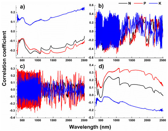
Figure 6.
Pearson correlation coefficients between soil nutrient contents and four spectral indices: (a) raw spectral reflectance; (b) first derivative; (c) second derivative; and (d) reciprocal logarithmic.
Table 2.
The optimal spectral variables selected for prediction of three soil nutrients
3.2. Estimation and Accuracy Assessment of Soil Nutrient Contents for Soil Sample Points
In this study, the selected spectral variables were used as independent variables and each of the soil nutrient (TN, TP and TK) contents was used as the dependent variable. The PLSR, BPNN and GA-BPNN models were compared to predict the contents of soil TN, TP and TK, respectively. In order to assess the quality of the prediction models for estimating the soil TN, TP and TK contents, the coefficient of determination (R2) and relative root mean square error (RRMSE) between the estimated and observed values and ratio of performance to deviation (RPD) were calculated based on both the modeling dataset and test dataset. In this study, the RPD is defined as the ratio of standard deviation to RMSE. The higher the RPD value, the higher the quality of the prediction models. Generally, the values of RPD less than 1.4, from 1.4 to 2.0 and greater than 2.0 indicate the poorest, fairly acceptable and accurate predictive performance, respectively [44,45]. The obtained PLSR prediction models are:
In this study, moreover, a three-layer BPNN with a single hidden layer was used to predict the soil nutrient contents. The number of neuron nodes in the hidden layer was set up as 13, the number of iterations was set up as 1000, and both the learning rate and learning objective were set up as 0.01. In order to compare the results of the GA optimization, the network structure and parameter configuration were the same as those in the BPNN. In the GA, the number of the maximum runs was set up as 20, and the population size, crossover probability () and mutation probability () were respectively set up as 128, 0.9 and 0.02. For the PLSR, BPNN and GA-BPNN, 50 training samples were selected to train the response relationships of the soil nutrient contents with the optimal spectral variables (Figure 7).
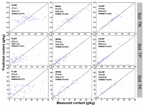
Figure 7.
Scatterplots of measured versus predicted values of the soil nutrient contents obtained by partial least squares regression (PLSR), BPNN and GA-BPNN (R2: coefficient of determination; RRMSE: relative root mean square error; RPD: ratio of performance to deviation).
Based on the modeling dataset, the explanatory power of the soil TN varied greatly depending on the prediction models and increased from 10.91% by PLSR to 83.89% by BPNN and 87.61% by GA-BPNN. The similar trends happened to soil TP and TK. The explanatory power of the soil TP increased from 30.88% by PLSR to 82.06% by BPNN and 94.25% by GA-BPNN, and the explanatory power of soil TK increased from 21.48% by PLSR to 92.18% by BPNN and 96.25% by GA-BPNN. Given a soil nutrient, the RRMSE values of the model predictions decreased, while the RPD values increased from PLSR to BPNN and GA-BPNN. The differences in the decrease of RRMSE and increase of RPD were great between the PLSR and BPNN or GA-BPNN and small between the BPNN and GA-BPNN. The modeling accuracy of the linear PLSR model was obviously much lower than those by two nonlinear models BPNN and GA-BPNN, implying that there existed a significant nonlinear relationship between the spectral variables and the soil nutrient contents.
Moreover, 25 soil samples were used to validate the prediction accuracy of three models. The validation results are shown in Figure 8, where the predicted values of the soil nutrient contents were plotted against the measured values, implying that GA-BPNN had a more powerful ability for the prediction of the soil nutrient contents because its scatter plot was closer to the 1:1 line than those from PLSR and BPNN. The predicted values of the PLSR model were significantly different from the measured values with large biases of the scatter points in the 1:1 line, indicating that obvious overestimations and underestimations occurred for the smaller and larger values, respectively. That is, the prediction ability of the PLSR model was poor for all three soil nutrients.
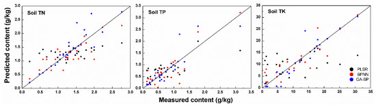
Figure 8.
The scatter plots of the predicted versus measured soil nutrient contents (TN, TP and TK) using the validation dataset.
In Table 3, the PLSR model led to the poorest estimates with the smallest values of R2 and RPD and the greatest values of RRMSE, while the GA-BPNN model showed the most accurate estimates with largest values of R2 and RPD and smallest values of RRMSE for all three soil nutrient contents. The validation results further indicated that the GA-BPNN models provided the best performance for estimating the soil nutrient contents.
Table 3.
The prediction accuracies of soil nutrient contents using PLSR, BPNN and GA-BPNN methods based on the validation dataset (R2: coefficient of determination; RRMSE: relative root mean square error; RPD: ratio of performance to deviation).
3.3. Estimation and Accuracy Assessment of Soil Nutrient Contents at the Regional Scale
In order to obtain more accurate values of spectral reflectance, Equation (9) was applied to derive the fractions of vegetation canopy and soil using the HJ-1A HSI band 848 nm in Figure 9. Then, the soil spectral reflectance was retrieved according to the area fraction of soil in Figure 10.
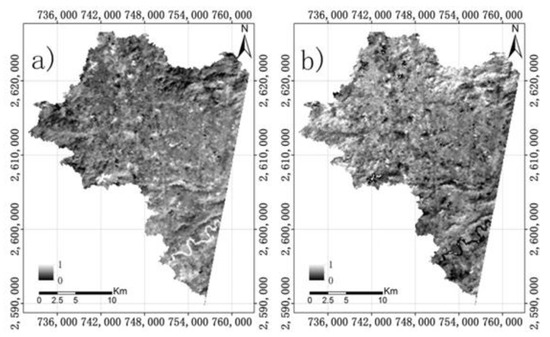
Figure 9.
The area fractions of (a) soil and (b) vegetation derived from the HJ-1A HIS band 848 nm using a linear spectral unmixing analysis for the study area.
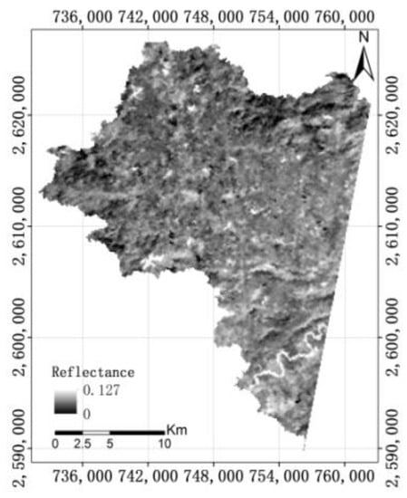
Figure 10.
Spectral reflectance of soil at band 848 nm of HJ-1A HIS image.
Based on the hyperspectral data collected in the laboratory, the lab-derived GA-BPNN had the best performance of the predictions for the soil nutrient contents. In this study, three lab-derived models including PLSR, BPNN and GA-BPNN were further compared by applying them to mapping the contents of the soil nutrients (TN, TP and TK) using the optimal spectral variables from the HJ-1A HIS image for the Conghua district at the regional scale. To obtain the optimal spectral variables, the HJ-1A HSI spectral data were first selected and re-sampled to estimate the soil nutrient contents, which led to the original optimal spectral variables (OOSV), including band 562, band 574 and band 591 for TN; band 603, band 613 and band 650 for TP; and band 625, band 802 and band 892 for TK. From the bands, the soil component reflectance values of mixed pixels were then derived using the linear spectral unmixing analysis, which led to the soil component optimal spectral variables (SCOSV). The results of applying the optimal spectral variables to the lab-derived models showed that the spatial distributions of the soil nutrient contents obtained by BPNN and GA-BPNN presented very similar spatial patterns, while the prediction maps of the soil nutrient contents using PLSR looked very different and unreasonable with much greater values throughout the whole area. Moreover, the prediction accuracies of the lab-derived models at the regional scale were assessed using the measurements of the soil nutrient contents from 33 soil samples in Conghua district. When the set of the SCOSV optimal spectral variables was used, the obtained RRMSE values by PLSR, BPNN and GA-BPNN were 82.37%, 50.56% and 40.41% for TN; 57.50%, 41.65%, 34.71% for TP; and 71.62%, 38.52% and 20.37% for TK. This indicated that the GA-BPNN models created the most accurate estimates for all the soil nutrient contents, and the BPNN models and the PLSR had the poorest performance. Similar results were obtained when the set of the OOSV optimal spectral variables was utilized. However, given a model, the set of the SCOSV optimal spectral variables after the decomposition of mixed pixels resulted in more accurate predictions of all the soil nutrient contents than the set of the OOSV before the decomposition of mixed pixels. Due to the limited space, the figure and table were omitted.
The spatial distributions of the predicted soil nutrient contents from the OOSV-based GA-BPNN model and the SCOSV-based GA-BPNN model were compared in Figure 11. Given a soil nutrient, two sets of the optimal spectral variables, OOSV and SCOSV, led to similar spatial patterns of the predictions. Table 4 showed the comparison of the predicted soil nutrient contents from the OOSV-based GA-BPNN model and the SCOSV-based GA-BPNN model based on the measurements of the soil nutrient contents from the 33 test samples in the Conghua district at the regional scale. The SCOSV-based GA-BPNN model led to more accurate estimates of all the soil nutrient contents than the OOSV-based GA-BPNN model. However, the prediction accuracies of the soil nutrient contents for Conghua district at the regional scale using the GA-BPNN model were obviously lower than those from the GA-BPNN model for Guangdong province at the sample point level. Compatibly, the soil TK content showed higher estimation accuracy with R2 = 0.80 and RRMSE = 20.37% than the soil TN with R2 = 0.58 and RRMSE = 40.41% and the soil TP with R2 = 0.69 and RRMSE = 34.71%, indicating that the SCOSV-based GA-BPNN model was capable of mapping the soil TK content using the HJ-1A HSI data at the regional scale.
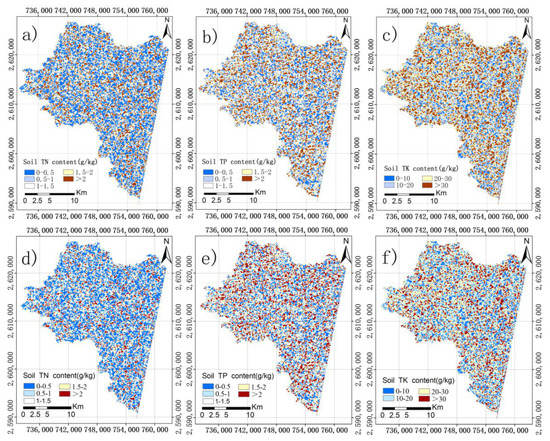
Figure 11.
Spatial distributions of soil nutrient contents for the testing area: (a) and (d) TN maps acquired from the original optimal spectral variables (OOSV) and the soil component optimal spectral variables (SCOSV); (b) and (e)TP map acquired from the OOSV and SCOSV; and (c) and (f) TK maps obtained from the OOSV and SCOSV.
Table 4.
Comparison of measured and predicted contents of TN, TP, and TK obtained using the original optimal spectral variables (OOSV) based GA-BPNN model and the soil component optimal spectral variables (SCOSV) based GA-BPNN model based on the 33 validation sample plots (St. Dev: standard deviation; R2: coefficient of determination; RRMSE: relative root mean square error).
4. Discussion
Soil nutrients, such as TN, TP, and TK, play a vital role in plant growth. Accurately estimating and mapping soil nutrient contents and monitoring their dynamics become critical. Estimating soil nutrient contents in soils using hyperspectral data is a cost-efficient but challenging method due to the effects of complex landscapes, vegetation canopies, mixed pixels and soil properties [41].
Previous studies [20,21,22,23,24] demonstrated that the BPNN method was a good alternative to estimating the soil nutrient contents with the values of R2 varying from 0.65 to 0.85 for TN, 0.60 to 0.75 for TP and 0.62 to 0.85 for TK, being often obtained. In this study, the corresponding R2 values obtained from the BPNN models without the integration of GA were 0.65, 0.74 and 0.81 for the soil nutrient TN, TP and TK contents, respectively (Table 3). This indicated that the research results driven from the BPNN models are in agreement with the findings of previous studies.
However, the large uncertainties of the input initial parameters for BPNN affected the improvement of estimation accuracy for the contents of soil nutrients [25]. In this study, GA was introduced to BPNN, which led to an integrated GA-BPNN method to optimize the BPNN initial input parameters (thresholds and weights) and provide the solution for the problem of being stuck in the local minima [46]. The results of the test datasets in this study showed that compared with the BPNN models without the optimization of the input parameters, the GA-BPNN models significantly improved the estimation accuracies of the soil nutrient contents by decreasing the RRMSE values by 15.9%, 5.6% and 20.2% at the sample point level, and 20.1%, 16.5% and 47.1% at the regional scale for TN, TP and TK, respectively.
In addition, in order to validate the regional scale applicability of the GA-BPNN prediction models, the HJ-1A HSI data (including OOSV and SCOSV) were used to map the soil nutrient contents for Conghua district. The results of validation using the 33 soil samples showed that the GA-BPNN models provided the potential to map the soil nutrient contents, but the TK content was more reliably estimated than the TN and TP contents, implying that the GA-BPNN was capable of estimating the soil TK content at the regional scale using HJ-1A HSI image. The SCOSV-based GA-BPNN model led to higher prediction accuracies than the OOSV-based GA-BPNN model at the regional scale, which may be attributed to reducing the effects of vegetation cover. However, compared with that using the measured hyperspectral data in laboratory, the prediction accuracy of the soil nutrient contents using the HJ-1A HSI image was lower, which might be attributed to the atmospheric conditions, soil surface conditions (e.g., soil moisture), and inconsistent band ranges between the spectral data of lab-measurement and hyperspectral image [47]. Thus, these factors should be considered in future research.
In order to obtain more accurate predictions for soil nutrient contents, we will add other prediction methods (e.g., MLP, deep learning, SVM and RF, etc.). In addition, in this study we only used 50 soil samples to build the prediction models and 25 soil samples to validate the model predictions in the whole Guangdong province. Although the sampling design was conducted based on soil types, the sample sizes were relatively small. However, the study focused on developing high-accuracy prediction methods rather than spatial mapping. Thus, the sample sizes were statistically acceptable. In the future studies, larger sample sizes should be utilized to further build and validate the prediction methods.
5. Conclusions
This study focused on the development and assessment of the GA-BPNN method for soil spectroscopy analysis to predict the contents of soil nutrients TN, TP and TK, using the hyperspectral measurements from soil samples taken from Guangdong, China, and collected in a laboratory. To validate the results, a comparison with two other commonly used methods (PLSR and BPNN) was made. Moreover, the lab-driven models were assessed by their applications to the Conghua district of Guangzhou City to map the contents of the soil nutrients at the regional scale using HJ-1A HSI image. To the best of our knowledge, this is the first time that GA-was integrated with BPNN for predictions of the soil nutrient contents. The results revealed that (1) Based on the RRMSE values from the validation datasets, the GA-BPNN models of the soil nutrient contents offered the most accurate estimates at both the soil sample point level and the regional scale; (2) Compared with BPNN models without GA, the GA-BPNN models significantly decreased the RRMSE values of all the predicted soil nutrient contents, implying that by integrating GA to optimize the parameters of BPNN, the GA-BPNN provided greater potential to improving the estimation; (3) The prediction accuracies of PLSR models were much lower than those from the BPNN and GA-BPNN models. This implied that there existed a significantly nonlinear relationship between the spectral variables and the soil nutrient contents; (4) The content of TK could be reliably mapped by the GA-BPNN method, with RRMSE values of 20.37% for the Conghua district at the regional scale, while the contents of soil TN and TP were relatively difficult to predict with the RRMSE values of 40.41% and 34.71% at the regional scale. The results provided a reliable reference for the optimization of the spectral prediction models and the improvement for the prediction accuracy of the soil nutrient contents at the regional scale.
Author Contributions
Y.P. and Z.L. conceived and designed the experiments; Y.P., L.W., L.Z., and Y.H. performed the experiments; Y.P. analyzed the data and wrote the draft of the manuscript; Z.L. and G.W. revised the manuscript.
Funding
This research was supported by the National Key Research and Development Program of China (2016YFC0501801, 2018YFD1100801-01), Qinghai Province Science and Technology Planning Project (2017-ZJ-730) and the Guangzhou Science and Technology Project, China (201804020034).
Acknowledgments
We gratefully acknowledge the paper writing assistance of Tao Ma as well as the experimental assistance of Ting Wang and Ziqing Xia.
Conflicts of Interest
The authors declare no conflict of interest.
References
- Chen, L.F.; He, Z.B.; Du, J.; Yang, J.J.; Zhu, X. Response of soil carbon cycling to climate warming: Challenges and perspectives. Acta Prataculturae Sin. 2015, 24, 183–194. [Google Scholar]
- Dong, X.; Tian, J.; Zhang, R.H.; He, D.X.; Chen, Q.M. Study on the Relationship between Soil Emissivity Spectra and Content of Soil Elements. Spectrosc. Spectr. Anal. 2017, 37, 557–565. [Google Scholar]
- Liu, P.; Liu, Z.; Hu, Y.; Shi, Z.; Pan, Y.; Wang, L.; Wang, G. Integrating a Hybrid Back Propagation Neural Network and Particle Swarm Optimization for Estimating Soil Heavy Metal Contents Using Hyperspectral Data. Sustainability 2019, 11, 419. [Google Scholar] [CrossRef]
- Hively, W.D.; Mccarty, G.W.; Reeves, J.B.; Lang, M.W.; Oesterling, R.A.; Delwiche, S.R. Use of Airborne Hyperspectral Imagery to Map Soil Properties in Tilled Agricultural Fields. Appl. Environ. Soil Sci. 2011, 2011, 1–13. [Google Scholar] [CrossRef]
- Gao, H.Z.; Lu, Q.P. Near infrared spectral analysis and measuring system for primary nutrient of soil. Spectroscopy and Spectral Analysis 2011, 31, 1245–1249. [Google Scholar]
- Xu, Y.M.; Smith, S.E.; Grunwald, S.; Abd-Elrahman, A.; Wani, S.P. Effects of image pan sharpening on soil total nitrogen prediction models in South India. Geoderma 2018, 320, 52–66. [Google Scholar] [CrossRef]
- Cao, F.X.; Yang, Z.J.; Ren, J.C.; Jiang, M.Y.; Ling, W.K. Linear vs. Nonlinear Extreme Learning Machine for Spectral-Spatial Classification of Hyperspectral Images. Sensors 2017, 17, 2603. [Google Scholar] [CrossRef]
- Leone, A.P.; Viscarra-Rossel, R.A.; Amenta, P.; Buondonno, A. Prediction of Soil Properties with PLSR and vis-NIR Spectroscopy: Application to Mediterranean Soils from Southern Italy. Curr. Anal. Chem. 2012, 8, 283–299. [Google Scholar] [CrossRef]
- Casa, R.; Castaldi, F.; Pascucci, S.; Basso, B.; Pignatti, S. Geophysical and Hyperspectral Data Fusion Techniques for In-Field Estimation of Soil Properties. Vadose Zone J. 2013, 12, 1–10. [Google Scholar] [CrossRef]
- Chen, T.; Chang, Q.; Liu, J.; Clevers, J.; Kooistra, L.; Clevers, J. Identification of soil heavy metal sources and improvement in spatial mapping based on soil spectral information: A case study in northwest China. Sci. Total Environ. 2016, 565, 155–164. [Google Scholar] [CrossRef]
- Hu, G.; Sudduth, K.A.; He, D.; Myers, D.B.; Nathan, M.V. Soil Phosphorus and Potassium Estimation by Reflectance Spectroscopy. Trans. ASABE 2016, 59, 97–105. [Google Scholar]
- Ramoelo, A.; Skidmore, A.; Cho, M.A.; Mathieu, R.; Heitkönig, I.; Dudeni-Tlhone, N.; Schlerf, M.; Prins, H. Non-linear partial least square regression increases the estimation accuracy of grass nitrogen and phosphorus using in situ hyperspectral and environmental data. ISPRS J. Photogramm. Remote Sens. 2013, 82, 27–40. [Google Scholar] [CrossRef]
- Mouazen, A.; Maleki, M.; De Baerdemaeker, J.; Ramon, H. On-line measurement of some selected soil properties using a VIS–NIR sensor. Soil Tillage Res. 2007, 93, 13–27. [Google Scholar] [CrossRef]
- Liu, H.Z.; Shi, T.Z.; Chen, Y.Y.; Wang, J.J.; Fei, T.; Wu, G.F. Improving Spectral Estimation of Soil Organic Carbon Content through Semi-Superv ised Regression. Remote Sens. 2017, 9, 29. [Google Scholar] [CrossRef]
- Ma, W.B.; Tan, K.; Li, H.D.; Yan, Q.W. Hyperspectral Inversion of Heavy Metals in Soil of a Mining Area Using Extreme Learning Machine. J. Ecol. Rural Environ. 2016, 32, 213–218. [Google Scholar]
- Balabin, R.M.; Lomakina, E.I. Support vector machine regression (SVR/LS-SVM)—An alternative to neural networks (ANN) for analytical chemistry? Comparison of nonlinear methods on near infrared (NIR) spectroscopy data. Analyst 2011, 136, 1703–1712. [Google Scholar] [CrossRef]
- Tang, F.; Chen, M.; Wang, Z. New approach to training support vector machine. J. Syst. Eng. Electron. 2006, 17, 200–219. [Google Scholar]
- Ma, L.; Chen, C.; Shen, Y.; Wu, L.F.; Huang, Z.L.; Cao, H.L. Determinants of tree survival at local scale in a sub-tropical forest. Ecol. Res. 2014, 29, 69–80. [Google Scholar] [CrossRef]
- Falahatkar, S.; Hosseini, S.M.; Ayoubi, S.; Salmanmahiny, A. Predicting soil organic carbon density using auxiliary environmental variables in northern Iran. Arch. Agron. Soil Sci. 2016, 62, 375–393. [Google Scholar] [CrossRef]
- Song, Y.Q.; Zhao, X.; Su, H.Y.; Li, B.; Hu, Y.M.; Cui, X.S. Predicting Spatial Variations in Soil Nutrients with Hyperspectral Remote Sensing at Regional Scale. Sensors 2018, 18, 3086. [Google Scholar] [CrossRef]
- Yu, L.; Hong, Y.S.; Zhou, Y.; Zhu, Q. Inversion of Soil Organic Matter Content Using Hyperspectral Data Based on Continuous Wavelet Transformation. Spectrosc. Spectr. Anal. 2016, 36, 1428–1433. [Google Scholar]
- Mouazen, A.; Kuang, B.; De Baerdemaeker, J.; Ramon, H. Comparison among principal component, partial least squares and back propagation neural network analyses for accuracy of measurement of selected soil properties with visible and near infrared spectroscopy. Geoderma 2010, 158, 23–31. [Google Scholar] [CrossRef]
- An, X.F.; Wu, G.W.; Dong, J.J.; Guo, J.H.; Meng, Z.J. Study on the Prediction Model Based on a Portable Soil TN Detector. In Computer and Computing Technologies in Agriculture IX; Springer International Publishing: Cham, Switzerland, 2015; pp. 117–126. [Google Scholar]
- Xu, S.X.; Zhao, Y.C.; Wang, M.Y.; Shi, X.Z. Comparison of multivariate methods for estimating selected soil properties from intact soil cores of paddy fields by Vis–NIR spectroscopy. Geoderma 2018, 310, 29–43. [Google Scholar] [CrossRef]
- Wang, F.; Gao, J.; Zha, Y. Hyperspectral sensing of heavy metals in soil and vegetation: Feasibility and challenges. ISPRS J. Photogramm. Remote Sens. 2018, 136, 73–84. [Google Scholar] [CrossRef]
- Wang, Q.; Wu, C.; Li, Q.; Li, J. Chinese HJ-1A/B satellites and data characteristics. Sci. China Earth Sci. 2010, 53, 51–57. [Google Scholar] [CrossRef]
- Walkley, A.J.; Black, C.A. An estimation of the Degtjareff method for determining soil organic matter and a proposed modification of the chromic acid titration method. Soil Sci. 1934, 37, 29–38. [Google Scholar] [CrossRef]
- Wang, J.; Cui, L.; Gao, W.; Shi, T.; Chen, Y.; Gao, Y. Prediction of low heavy metal concentrations in agricultural soils using visible and near-infrared reflectance spectroscopy. Geoderma 2014, 216, 1–9. [Google Scholar] [CrossRef]
- Gomez, C.; Lagacherie, P.; Coulouma, G. Continuum removal versus PLSR method for clay and calcium carbonate content estimation from laboratory and airborne hyperspectral measurements. Geoderma 2008, 148, 141–148. [Google Scholar] [CrossRef]
- Adeline, K.; Gomez, C.; Gorretta, N.; Roger, J.-M. Predictive ability of soil properties to spectral degradation from laboratory Vis-NIR spectroscopy data. Geoderma 2017, 288, 143–153. [Google Scholar] [CrossRef]
- Fabre, S.; Briottet, X.; Lesaignoux, A. Estimation of Soil Moisture Content from the Spectral Reflectance of Bare Soils in the 0.4-2.5 µm Domain. Sensors 2015, 15, 3262–3281. [Google Scholar] [CrossRef]
- Lin, L.X.; Wang, Y.J.; Teng, J.Y.; Xi, X.X. Hyperspectral Analysis of Soil Total Nitrogen in Subsided Land Using the Local Correlation Maximization-Complementary Superiority (LCMCS) Method. Sensors 2015, 15, 17990–18011. [Google Scholar] [CrossRef] [PubMed]
- Zhao, L.; Hu, Y.-M.; Zhou, W.; Liu, Z.-H.; Pan, Y.-C.; Shi, Z.; Wang, L.; Wang, G.-X. Estimation Methods for Soil Mercury Content Using Hyperspectral Remote Sensing. Sustainablity 2018, 10, 2474. [Google Scholar] [CrossRef]
- Salmerón Gómez, R.; García Pérez, J.; López Martín, M.D.M.; García, C.G. Collinearity diagnostic applied in ridge estimation through the variance inflation factor. J. Appl. Stat. 2016, 43, 1831–1849. [Google Scholar] [CrossRef]
- Kang, J.; Jin, R.; Li, X.; Zhang, Y.; Zhu, Z. Spatial Upscaling of Sparse Soil Moisture Observations Based on Ridge Regression. Remote Sens. 2018, 10, 192. [Google Scholar] [CrossRef]
- Wold, H. Nonlinear Estimation by Iterative Least Squares Procedure. In Research Papers in Statistics; David, F., Ed.; Wiley: Hoboken, NJ, USA, 1966; pp. 441–444. [Google Scholar]
- Wold, S.; Sjöström, M.; Eriksson, L. PLS-regression: A basic tool of chemometrics. Chemometr. Intell. Lab. 2001, 58, 109–130. [Google Scholar] [CrossRef]
- Duan, S.M. Design and Development of Detection Node in Wireless Sensor Network Based on Neural Network. Adv. Mater. Res. 2014, 1022, 292–295. [Google Scholar] [CrossRef]
- Panda, S.S.; Ames, D.P.; Panigrahi, S. Application of Vegetation Indices for Agricultural Crop Yield Prediction Using Neural Network Techniques. Remote Sens. 2010, 2, 673–696. [Google Scholar] [CrossRef]
- Haque, M. ANN back-propagation prediction model for fracture toughness in microalloy steel. Int. J. Fatigue 2002, 24, 1003–1010. [Google Scholar] [CrossRef]
- Lu, P.; Wang, L.; Niu, Z.; Li, L.; Zhang, W. Prediction of soil properties using laboratory VIS–NIR spectroscopy and Hyperion imagery. J. Geochem. Explor. 2013, 132, 26–33. [Google Scholar] [CrossRef]
- Saleh, S.; Ibrahim, K.; Eiteba, M.M.; Mohamed, S. Study of genetic algorithm performance through design of multi-step LC compensator for time-varying nonlinear loads. Appl. Soft Comput. 2016, 48, 535–545. [Google Scholar] [CrossRef]
- Keshava, N.; Mustard, J.F. Spectral unmixing. IEEE Signal Process. Mag. 2002, 19, 44–57. [Google Scholar] [CrossRef]
- Pirie, A.; Singh, B.; Islam, K. Ultra-violet, visible, near-infrared and mid-infrared diffuse reflectance spectroscopis techniques to predict several soil properties. Aust. J. Soil Res. 2005, 43, 713–772. [Google Scholar] [CrossRef]
- Razakamanarivo, R.H.; Grinand, C.; Razafindrakoto, M.A.; Bernoux, M.; Albrecht, A. Mapping organic carbon stocks in eucalyptus plantations of the central highlands of Madagascar: A multiple regression approach. Geoderma 2011, 162, 335–346. [Google Scholar] [CrossRef]
- Khosravi, V.; Ardejani, F.D.; Yousefi, S.; Aryafar, A. Monitoring soil lead and zinc contents via combination of spectroscopy with extreme learning machine and other data mining methods. Geoderma 2018, 318, 29–41. [Google Scholar] [CrossRef]
- Liu, Z.; Lu, Y.; Peng, Y.; Zhao, L.; Wang, G.; Hu, Y. Estimation of Soil Heavy Metal Content Using Hyperspectral Data. Remote Sens. 2019, 11, 1464. [Google Scholar] [CrossRef]
© 2019 by the authors. Licensee MDPI, Basel, Switzerland. This article is an open access article distributed under the terms and conditions of the Creative Commons Attribution (CC BY) license (http://creativecommons.org/licenses/by/4.0/).