Abstract
Criminal activities are often unevenly distributed over space. The literature shows that the occurrence of crime is frequently concentrated in particular neighbourhoods and is related to a variety of socioeconomic and crime opportunity factors. This study explores the broad patterning of property and violent crime among different socio-economic stratums and across space by examining the neighbourhood socioeconomic conditions and individual characteristics of offenders associated with crime in the city of Toronto, which consists of 140 neighbourhoods. Despite being the largest urban centre in Canada, with a fast-growing population, Toronto is under-studied in crime analysis from a spatial perspective. In this study, both property and violent crime data sets from the years 2014 to 2016 and census-based Ontario-Marginalisation index are analysed using spatial and quantitative methods. Spatial techniques such as Local Moran’s I are applied to analyse the spatial distribution of criminal activity while accounting for spatial autocorrelation. Distance-to-crime is measured to explore the spatial behaviour of criminal activity. Ordinary Least Squares (OLS) linear regression is conducted to explore the ways in which individual and neighbourhood demographic characteristics relate to crime rates at the neighbourhood level. Geographically Weighted Regression (GWR) is used to further our understanding of the spatially varying relationships between crime and the independent variables included in the OLS model. Property and violent crime across the three years of the study show a similar distribution of significant crime hot spots in the core, northwest, and east end of the city. The OLS model indicates offender-related demographics (i.e., age, marital status) to be a significant predictor of both types of crime, but in different ways. Neighbourhood contextual variables are measured by the four dimensions of the Ontario-Marginalisation Index. They are significantly associated with violent and property crime in different ways. The GWR is a more suitable model to explain the variations in observed property crime rates across different neighbourhoods. It also identifies spatial non-stationarity in relationships. The study provides implications for crime prevention and security through an enhanced understanding of crime patterns and factors. It points to the need for safe neighbourhoods, to be built not only by the law enforcement sector but by a wide range of social and economic sectors and services.
1. Introduction
Crime activities are often unevenly distributed over space in a municipality or geographic region [1], and the occurrence of crime tends to concentrate in particular neighbourhoods or settings [2,3,4,5]. Crime mapping using a Geographic Information System (GIS) has advanced greatly in recent years as a tool for increasing our understanding of crime patterns; it has replaced the “spot map” used by police forces, whereby pins are placed physically on large street maps to identify crime hazards [6]. In addition to the mapping approach, spatial statistical analytics has been applied to examine the concentration and dispersion of criminal activities, as well as the relationships between crime patterns and the socioeconomic characteristics of neighbourhoods and of both offenders and victims. For example, spatial clustering techniques are used to identify areas of high (or low) risk for drug offences that are surrounded by areas of non-random similar (or dissimilar) risks [4]. Such approaches allow for the identification of statistically significant “hot spots” or “cold spots” for various types of crime in a study area, providing critical insights into the socioeconomic and spatial contexts of criminal activities and crime patterns. Research has also found that neighbourhoods with high crime rates are associated with higher levels of economic disadvantage, larger proportions of young people, and greater residential instability [5]. Deprivation, a key measure of socioeconomic disadvantage, is found to be a robust determinant of crime rates at the neighbourhood level in urban settings or in large spatial units such as cities [7].
Identifying factors that contribute to the incidence of crime has been a central focus of research on crime occurrence and patterns. Offenders’ individual characteristics, such as education, gender, age, marital status, social class, and employment status, have been found to significantly relate to certain types of crime [8]. For example, the less educated are more likely to be engaged in crime compared to those with higher education; specifically, those with no more than a high school diploma are more likely to be incarcerated for fraud or drug-related crimes [9]. Gender and age interact to affect various types of crime. A Finnish study found that males and those in the 15-to-30 age cohort had a high prevalence of both property and violent crime [10]. In contrast, a regional study in Russia found more female offenders convicted of violent crimes as opposed to commercial or drug-related crime [11]. Furthermore, lifestyle theory suggests that the occurrence of crime is related to demographic variables because such characteristics are related to the offender’s lifestyle [12]. Lifestyle theory also relates to behaviour in terms of the characteristics of offenders’ daily routine, such as work, school, housing conditions, and leisure activities [13]. For example, marriage status and low income have been found to be positively related to burglary victimisation, while living in a detached house has been found to be negatively related [12].
A noticeable trend in crime research is the increasing influence of the social, economic, and political environments (i.e., contextual factors) on variations in neighbourhood crime. Research examining the association between neighbourhood contextual effects on crime has been largely built on social disorganisation theory, a key theoretical perspective linking the ecological characteristics of environment, such as economic disadvantage and ethnic heterogeneity, to neighbourhood crime occurrence [14,15]. Neighbourhoods at a high level of disadvantage in aspects such as poverty and unemployment often experience more crime due to there being fewer available resources to counteract it [2,7,16,17]. Resources may be particularly limited in geographically clustered disadvantaged neighbourhoods within disadvantaged cities or regions, resulting in higher rates of crime, particularly violent and property crime [7]. Neighbourhood environment can be approached by examining both the neighbourhood where the crime takes place and the neighbourhood where the offender resides. The neighbourhood may or may not be the same. Let us take the offender’s residential neighbourhood environment, for example. The land use pattern, represented by open areas and road density, has been found to be an important factor in youth crime [15]. Relative deprivation theory is concerned with the potential influence of neighbourhood environment on crime and the role of perceived inequality by individuals who compare themselves to the “reference group”; perceived inequitable income or share of resources, for example, as measured by the extent of income inequality, may cause stress or frustration, leading an individual to respond by engaging in criminal behaviour [18,19]. While it is a challenge to identify the proper reference group in order to determine relative inequality or deprivation an individual may feel, research has used residential neighbourhood and the larger city to explore the relationship between neighbourhood inequality and neighbourhood crime [7,20].
Routine activity theory offers an alternative framework for understanding crime occurrence when a motivated person encounters an opportunity (or a suitable target) in the absence of a capable guardian [21]. For example, property crime may increase when potential offenders routinely travel from their own neighbourhoods to more affluent (or less affluent) ones and become aware of the changed environment. Routine activity theory provides important spatial means of understanding the relationship between crime location and offender location and the spatial (or travel) behaviour associated with criminal activity.
Relatively little research has incorporated both contextual factors (e.g., neighbourhood socioeconomic conditions and environment) and individual (e.g., offender) characteristics in major crime analysis. Studies that focus on the influence of the neighbourhood (or city) context on crime often use contextual variables from census-based measures of deprivation or measures of other attributes such as alcohol outlet density, at a neighbourhood level, in order to identify the association between the neighbourhood environment and crime rates [5,16,22]. These studies feature a prominent spatial dimension, as criminal activities often cluster in socioeconomically marginalised or deprived areas. Studies that investigate the relationship between crime and individual characteristics of the offender are less geographical; they rely more on statistical analysis, such as regression [10]), due partly to the challenge of accessing small-scale geo-referenced, or spatial, data on crime (or victim) that also provide information on the socioeconomic characteristics of the individuals concerned.
This study seeks to determine both neighbourhood factors and individual characteristics of offenders associated with crime rates in Toronto. It employs spatial and quantitative methods to analyse two types of major crime: property crime and violent crime. The research literature indicates that property crime and violent crime have different spatial distributions and are associated with distinct neighbourhood characteristics—for example, those specific to Chicago [23]. There has been limited scholarly research conducted in Canada on crime spatial patterns and determinants relative to a specific type of crime. An exception is a cluster of studies conducted in the City of Vancouver that employs spatial and statistical techniques in investigating crime patterns and associated factors [24,25,26,27,28]. Although Toronto is the largest urban centre in Canada, with a fast-growing population, relatively little research has been conducted on the spatial distribution of different types of major crime in Toronto and their relationship to both contextual and offender characteristics. This study uses a diverse range of data sets, including geo-referenced data on property and violent crime and offender characteristics from 2014 and 2016, as well as 2006 Ontario Marginalisation (On-Marg) Index (the most recent On-Marg data at the neighbourhood level at the time of study), to shed light on the socioeconomic condition of neighbourhoods where crime occurs. The comparison between different factors associated with property crime and violent crime yields important implications for crime prevention and control related to the type of crime and the neighbourhood context.
2. Data
The study analyses two major spatial data sets in order to explore the spatial distribution and cluster patterns of crime incidence and the relationships among crime rates, offender characteristics, and neighbourhood context. The two data sets are at the city neighbourhood level, including major crime data obtained from the Business Intelligence and Analytics unit of the Toronto Police Service (TPS) and Ontario Marginalisation Index (On-Marg), a census-based dataset measuring multiple dimensions of marginalisation at the neighbourhood level for City of Toronto.
Due to the confidential nature of the data, and in accordance with the Municipal Freedom of Information and Protection of Privacy Act, according to which “local government institutions shall protect the privacy of an individual’s personal information existing in government records” [29], only aggregated crime data at the neighbourhood level is used in the study. There are, in total, 140 neighbourhoods in the City of Toronto. The crime data provides information on (a) the incidence of property and violent crime by neighbourhood in Toronto from 2014 to 2016; (b) select socioeconomic status (SES) (age, gender, marital status, distance travelled to crime location) of offenders charged with property and violent crime at the neighbourhood level; and (c) average distance travelled between offenders’ residence location and offence location. (i.e., journey to crime).
The SES variables allow us to understand the percentage of offenders per neighbourhood in various age groups, of different gender and marital status groups. The distance variable measures the average straight-line distance offenders travelled from their residential location to crime in a neighbourhood. It is calculated in Alteryx using the offender’s postal code location to the offence postal code location. In previous studies, the shortest distance is assumed to reduce travel costs and at the same time maximise the benefits of the criminal act [30,31,32]. The outputs are in kilometres and are classified among property and violent crimes to determine the differences among both groups. For confidentiality reasons, distance calculated at an individual level was aggregated to the neighbourhood level before it was analysed in the study. Calculated average distance travelled allows us to understand the behavioural differences between the spatial activity of property and violent crime, and is included in the regression models as a covariate.
Both property crime and violent crime are considered major crime indicators by the TPS. Property crime includes auto theft, break and enter, and other theft over $5000. Violent crime includes assault, robbery, and sexual assault. Murder and homicide accounted for less than 1% of all crime indicators in Toronto for each year from 2014 to 2016; they were excluded from the study because of their much lower rates. The focus on property crime and violent crime in the study is consistent with the literature; the two types of crime were studied separately due to differences in crime patterns related to seasonality, travel distance, and crime predictors [16,30,33].
The Ontario Marginalisation Index at the neighbourhood geography level allows us to understand the socioeconomic contexts of Toronto neighbourhoods [34]. It has four indices created from a total of 18 census variables to quantify four dimensions of marginalisation: residential instability, material deprivation, ethnic concentration, and dependency. These dimensions were defined using principal component factor analysis, which resulted in four factors with Eigenvalues greater than one [34]. Specifically, the deprivation index was derived from 6 census variables (population aged 25+ without a certificate, diploma or degree; lone-parent families; population receiving government transfer payments; population aged 15+ who are unemployed). The residential instability index was based on 7 census indicators (proportions of living alone, youth 5–15, multi-unit housing, married/common-law, dwellings owned, same house as 5 years ago, and average number of persons per dwelling). The ethnic concentration index was derived from 2 census variables (proportion of recent immigrants who arrived in the last five years and proportion of visible minorities). The dependency index is based on 3 census variables (proportion of seniors, dependency ratio, labour force participation ratio).
The study area—the City of Toronto—is located on the northwest shore of Lake Ontario. It consists of six census subdivisions: Etobicoke, York, North York, Toronto, East York, and Scarborough. It is the largest city in Canada, with a total population of 2,731,571, representing 8.7% of Canada’s population, 22.5% of Ontario’s population, and 43.8% of the population of the Toronto Census Metropolitan Area [35]. Toronto has a highly diverse population, demographically, socioeconomically, and culturally. Currently, the largest age group consists of those from 25 to 29 years and there are more people over the age of 65 than under the age of 15. More than 140 languages and dialects are spoken in the city and 51% of Torontonians identify as members of a visible minority. Approximately 20% of the population are below the low-income cut-offs (LICO), compared to 14% for Canada as a whole. According [36], rates of robbery, break-and-enter and auto theft rates for Toronto Census Metropolitan Area in 2010 were 128, 307 and 171 per 100,000, compared to 89, 577 and 272 in Canada. These rates were part of a general declining trend over more than a decade prior to 2010. Past research on crime patterns in Toronto has used the neighbourhood as a relevant spatial scale [5]. In Toronto, there are currently 140 neighbourhood profiles, with an average of some 4000 persons. Neighbourhood boundaries are delineated by the municipality of Toronto for planning purposes, using one or more Census Tract boundaries, which facilitates the use of Canadian Census data as the neighbourhood level geography is not collected by Statistics Canada. The neighbourhood is deemed an appropriate unit in the spatial analysis of crime in Toronto given its relatively homogenous socioeconomic characteristics and the confidential nature of crime data, which limits data access at finer spatial scales, including an individual level.
3. Methods
Measuring spatial patterning of crime. Crime rate is calculated by the total count of property crimes and violent crimes in neighbourhoods normalised by the total population of neighbourhoods at a rate of 100,000. This method, which has been used in Canada for many years, is critical to understanding the distribution of crime in a city without reporting disproportional values [37]. It also allows for systematic comparison between the spatial distribution of violent and property crime across a city in relation to neighbourhood socioeconomic inequalities. Past research has demonstrated the utility of ambient population over census-based residential population in analysing crime patterns and risk factors, in particular, in violent crime [28,38]. Ambient population is an estimate of the number of people in a given spatial unit at any time of the day and any day of the year, reflecting people’s daily and seasonal routine activities for employment, recreational and other purposes [24]. Ambient population data is however not always readily available in a study area and at a particular spatial scale. In a Vancouver-based study [24], while the use of ambient population in calculating violent crime rates had an impact on the results of spatial analysis relative to using residential population, the impact was greater for small geographies (i.e., DA) than in larger units (i.e., census tract). In these contexts, this paper uses census-based population data in measuring crime rates at the neighbourhood level.
To investigate the spatial distribution and clustering patterns of crime, Local Moran’s I, also known as Local Indicator of Spatial Association (LISA), is applied to explore the spatial autocorrelation among crime occurrences and identify hot and cold spots and spatial outliers [39]. It is an established spatial technique that has been used to explore clusters of various criminal offences, such as drug crimes and violent crimes [4,40,41]. The method identifies where high or low values cluster spatially and reveals features with values that are very different from those of surrounding features. In this study, first-order queen continuity is selected to define and interpret spatial relationships. This is because Toronto neighbourhoods are mostly irregularly shaped polygons, and neighbouring polygons are considered to be those sharing at least one point in common—border or vertex.
OLS regression and GWR models. An OLS (ordinary least square) multivariate regression model is first employed to explore the global relationship between the dependent variable and the independent variables. Property and violent crime are modelled separately. The dependent variable measures crime rates, per 100,000, for property crime and for violent crime. The independent variables include (1) the four dimensions of On-Marg Index (residential instability, material deprivation, ethnic concentration, and dependency) measuring neighbourhood socioeconomic conditions; and (2) key offender characteristics, including age, marital status, and average distance travelled to offence location. All variables are measured at the neighbourhood level. As a global regression technique, the OLS regression is an effective tool for exploring the relationship between crime rates and neighbourhood-level variables [2,5,42,43,44,45,46]. Similar variables have been found to be associated with crime [9,10,11,12].
OLS regression is run in Esri ArcGIS. The output returns diagnostic statistics on multicollinearity and spatial independency of residuals. Multicollinearity is assessed by examining the Variance Inflation Factor (VIF) values. Large VIF values (>7.5) in general indicate a redundancy among explanatory variables. The spatial independency of regression residuals is evaluated by using the spatial autocorrelation coefficient, Global Moran’s I [47]. The Global Moran’s I index falls between [−1, 1], where 1 describes a very strong positive autocorrelation (clustering) and −1 reflects a strong negative clustering pattern. If the value is close to 0, the pattern corresponds to a random arrangement [48,49]. This test also returns results for z-score and p-values indicating whether the results are statistically significant.
Spatial dependency (or autocorrelation) of residuals calls for using a geographically weighted regression (GWR) to further examine how the statistical relationship between dependent and independent variables varies over space [50,51]. GWR is a local form of OLS regression that allows the regression parameter estimation to change locally. In this study, it constructs a separate OLS equation for every neighbourhood in the City of Toronto by incorporating the dependent and independent variables associated with neighbourhoods that fall within a bandwidth of each target neighbourhood. Each neighbourhood (a feature in the dataset) is associated with its own parameter estimation. As such, GWR produces a set of parameter estimates and pseudo t-values of significance that vary over space. For each variable, Pseudo t-values and local coefficients are mapped out. The spatial variation of these parameter estimates sheds light on the ways in which crime rates are associated with spatially varying processes represented by different individual and neighbourhood contexts. Akaike Information Criterion (AIC) and adjusted R2 are generated for both OLS and GWR models as indicators of model fit and performance.
4. Findings and Results
From 2014 to 2016, there were 3419 and 21,999 persons in Toronto charged with property and violent crimes, respectively, under the Canadian Criminal Code (Table 1). The data does not provide additional information on whether the same individual is linked to multiple offenses, and it is possible that the offenders are in fact the same person for some crimes included. Table 2 describes the general demographic characteristics of those charged with property and violent crimes from 2014 to 2016. The 18-to-34 age group has the highest percentages for both types of offence. Percentages for male offenders are dramatically higher than those for female offenders. Percentages for single offenders are higher than those for partnered offenders. While other factors, such as income and ethnicity, are examined in the literature to understand the demographic composition of offenders, due to data confidentiality only these three characteristics (age, gender, and marital status) of offenders at an aggregated neighbourhood level are available to the study.

Table 1.
Number of offenders charged, 2014–2016.
Table 2.
Demographic characteristics of property and violent crime offenders, 2014–2016.
4.1. Spatial Distribution and Spatial Cluster of Crimes
Figure 1 depicts the spatial distribution of rates for property and violent crime from 2014 to 2016. There is a high concentration of both types of crime in the downtown core, northeast end (Etobicoke York, North York), and small pockets in the east end (Scarborough). Neighbourhoods that have some of the highest crime rates are West Humber-Clairville, Islington-City Centre West, York University Heights, Trinity-Bellwoods, and Woburn. There are lower concentrations of crime at the centre and lower west end of the city.
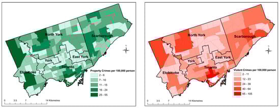
Figure 1.
Property and violent crime rates (per 100,000 persons) by Toronto neighbourhood, 2014–2016.
LISA statistics further enhance our understanding of the spatial distribution and clustering patterns of crime in the city of Toronto. The Global Moran’s I value of the LISA statistics is 0.27 for property crime (z-score = 6.96; p = 0.00) and 0.40 for violent crime (z-score = 10.23; p = 0.00), indicating no spatial independence in these data sets and a clustered spatial distribution of both criminal activities in Toronto. Figure 2a,b visually display the distribution of significant and insignificant spatial autocorrelation for property and violent crime, respectively. The maps highlight areas of relatively high and low significance for both property and violent crime. For both crime types, downtown Toronto has several fairly consistent high-high clusters where high crime rates are surrounded by high crime rates (i.e., positive spatial autocorrelation). One isolated high-high cluster of violent crime is seen in east Toronto (Scarborough). Low-low clusters of violent crimes are distinctly present in the centre of Toronto, with a few pockets in west Toronto (Etobicoke) and North York. High-low and low-high (negative spatial autocorrelation) are more spread out in the city, with high-low clusters mostly in west and central Toronto (Etobicoke and North York).

Figure 2.
(a) LISA Statistics Map for Property Crime, 2014–2016. (b) LISA Statistics Map for Violent Crime, 2014–2016.
4.2. The Distance-to-Crime Variable
The distance-to-crime measurement calculates the shortest distance travelled by the offender between their residential location and the corresponding crime location within Toronto. Acknowledging that the origin of the journey to crime is not necessarily home and that the spatial behaviour involved in criminal activity is far more complex than a straightforward travel pattern between home and crime locations, the distance computed provides a quick glimpse of where crime occurs in relation to the offender’s residential location. As shown in Table 3, the average distance travelled by violent crime offenders is 4.9 kilometres, compared to 7.6 kilometres for property crime offenders. The longest distance travelled was 49.2 kilometres for property offenders and 36.6 kilometres for violent crime offenders. This is consistent with the literature, which suggests a higher average travel distance among property offenders than among violent offenders [30].
Table 3.
Distance to crime.
4.3. OLS Results
OLS regression is employed to explore the statistical association between crime rates and the independent variables measuring offenders’ characteristics and neighbourhood socioeconomic context. Due to data availability, the regression is run at the neighbourhood level. Prior to conducting the OLS regression, multicollinearity is tested using a Pearson’s correlation diagnostic including all potential variables. Gender is excluded from the OLS regression because of its high correlation with age. The final list of independent variables and OLS regression results are provided in Table 4. None of the independent variables are found to be highly correlated with the others, nor with the crime rates with a correlation coefficient over 0.7 or higher. In addition, the VIF values reported in Table 4 are all under 7.5, indicating no multicollinearity that exits with the OLS estimation. In general, both offender characteristics (% age 18–34 and % couple) are significantly related to the independent variables; distance-to-crime shows a non-significant relation with either crime; different On-Marginalisation indices exhibit different relationships with crime rates for different crimes. More specifically, an increase in proportions of the 18-to-34 age group among offenders in neighbourhoods positively relates to an increase in violent crime rates, but negatively to property crime rates. Increase in proportion of offenders who were married/common law relates significantly to a decrease in violent crime rates, but an increase in property crime rates. Among the four dimensions of the Ontario Marginalisation index, neighbourhoods associated with a higher level of instability and deprivation are significantly associated with a higher level of violent crime rates. Neighbourhoods that have a higher level of instability and lower level of ethnic concentration are significantly related to higher property crime rates.
Table 4.
Ordinary Least Squares (OLS) regression results for violent and property crime, respectively (n = 140).
The adjusted R2 indicates that the models explained about 73% and 71% of the total variances of violent and property crime rates, respectively. However, the residuals of the OLS model for property crime reveal a significant positive spatial autocorrelation (Global Moran’s I = 0.20, p = 0.00), which violates the assumption of OLS on the independence of residuals. To address this limitation, a GWR model is used to further explore the relationship between property crime rates and the dependent variables. In the case of violent crime, the OLS residuals exhibit a random pattern, as diagnosed by Global Moran’s I test (Global Moran’s I = −0.08, p = 0.13). OLS is thus considered an adequate model in exploring the relationship between the independent variables and violent crime rates, and GWR is not required, as suggested by the literature [52]. Post-hoc analysis confirms that applying GWR to violent crime did not offer improved results and the adjusted R2 remains to be 0.73.
4.4. GWR for Property Crime
The results of the GWR for property crime are provided in Table 5. The coefficients of GWR are reported in terms of minimum, 25th percentile (or maximum of first quartile), 50th percentile (or maximum of second quartile), 75th percentile (or maximum of third quartile) and maximum values. The adjusted R2 of the GWR is 0.80, representing a 9% increase from that in the OLS regression. The GWR also produce decreased AICc. These model statistics indicate that the GWR is a more suitable model that can explain 80% of the variations in observed property crime rates across different neighbourhoods in Toronto. The condition numbers are all below the critical value of 30, indicating that the results are reliable and local multicollinearity is not an issue in the GWR model.
Table 5.
Geographical weighted regression (GWR) results for property crime.
Visualising the estimated locally weighted R2 allows for an understanding of how well the GWR model fits observed property crime rates in different areas. Figure 3 depicts the distribution of local R2, which is not distributed homogeneously across neighbourhoods. In general, GWR predicts well towards the western part of Toronto, with R2 values over 0.80. For example, Markland Wood, Long Branch and Alder Wood in Etobicoke are associated with R2 values over 0.86. Neighbourhoods in the western end of Toronto are associated with lower local R2 values. Some of the neighbourhoods in Scarborough, such as Highland Creek, Centennial Scarborough and West Hill, have the lowest R2 of 0.66 in the city. The low R2 suggests that additional covariates may play a role in affecting local crime activities in these neighbourhoods.
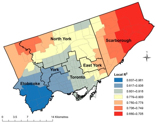
Figure 3.
Distribution of adjusted local R2 in GWR model for property crime.
In the GWR model, pseudo t statistics indicate the significance of locally varying coefficients for the independent variables. Figure 4 shows the spatial distribution of pseudo t-values for the intercept and each independent variables in the study area. Pseudo t is calculated by dividing coefficient estimate by the standard error, with significance (p < 0.05) defined as a pseudo t-value > 1.96 (positive relationship) or <−1.96 (negative relationship) [51,53,54,55]. Non-significant relationships are represented in yellow in Figure 4, with significant positive relationships in red/orange, and significant negative relationships in green/light green. Figure 5 visualises local coefficients for the intercept and independent variables in the GWR model. It essentially reveals how the direction and strength of the relationship between the independent and each dependent variable varies over space. Examining both pseudo t surface in Figure 4 and coefficient maps in Figure 5 yields useful insights into spatial variations in relationships. The spatial patterns of pseudo t and local coefficients are, in general, consistent with the OLS regression results in terms the direction of relationship; they also reveal fine spatial details in the local variation of the strength and direction of relationship. For example, age (18–34) and ethnic concentration exhibit a significantly negative relationship with crime rates in most Toronto neighbourhoods. Exceptions are the eastern part of Scarborough (for both variables) and western Etobicoke (for ethnic concentration), where the relationships are insignificant. Marital status (i.e., % couple) is significantly and positively related to crime rates in the vast majority of the city neighbourhoods, except for the eastern corner of Scarborough. In OLS regression, both deprivation and dependency are insignificant predictors of property crime rates. The GWR results however reveal a cluster of neighbourhoods in York, southeastern corner of North York and southwestern corner of Scarborough, where property crime rates exhibit a positive relationship with deprivation and a negative relationship with dependency in a significant way. The GWR finding complement the OLS results that do not reveal local details.
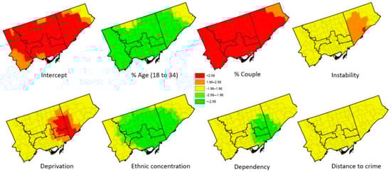
Figure 4.
Pseudo t-values for intercept and independent variables.
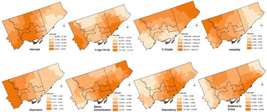
Figure 5.
GWR local coefficients for intercept and independent variables.
5. Discussion, Limitations, and Future Research
This paper explores the spatial patterning of property and violent crime at the neighbourhood level in Canada’s largest urban centre. It examines the ways in which select offender characteristics and neighbourhood socioeconomic conditions are associated with neighbourhood crime rates. By employing spatial analytical techniques in determining crime spatial variation and crime cluster, the study adds to the relatively small amount of Canadian literature on spatial crime analysis based on different types of major crime. Using a traditional global OLS regression and a geographically weighted regression (GWR), the study simultaneously considers the compositional effects resulting from differences in offenders and contextual effects resulting from differences between neighbourhoods in explaining variations in crime rates. By doing so, it contributes to the literature, which has tended to focus separately on the broader neighbourhood (or city) context and individual offender characteristics in predicting crime occurrence [5,10].
The spatial analyses confirm the results of scholarly research indicating that crime is not randomly distributed in space but, rather, concentrated in neighbourhoods that share particular characteristics [2,3]. As evidenced in Figure 2a,b, the spatial distribution of property crimes and violent crimes follows an approximate U-shaped pattern across the city, roughly aligning with neighbourhoods that have lower social economic status described in the U-shaped poverty corridor in Toronto [56,57]. The OLS and GWR models further confirm the significant relationship between crime rates (both property and violent) and various dimensions of the Ontario Marginalisation index. This echoes the social disorganisation theory linking crime with neighbourhood socioeconomic disadvantage [58]. Property and violent crimes tend to cluster in similar neighbourhoods over the three years of the study (2014–2016), with consistent concentrations of crime in the city core and high concentrations in the northwest and northeast parts of the city, especially with regard to property crime. In comparison to violent crime, property crime shows more dispersion across neighbourhoods. The LISA maps reveal statistically significant spatial clusters of both property and violent crime. While three years may not be long enough to yield substantial findings, the spatial distinction between property and violent crime is evident.
It should be noted that for each crime type, distance-to-crime is not a significant predictor of neighbourhood crime rates in the present study, which does not directly approve the routine activity theory. However, in comparing the two crime types, the distance-to-crime measurement reveals a longer distance travelled to crime location by property crime offenders than by violent crime offenders. This finding is similar to that reported by [30] suggesting a higher average travel distance among property offenders than among violent offenders. This has implications in understanding the routine activity theory, which indicates that crime is affected not only by the socioeconomic characteristics of offenders, but also by other potential factors such as an individual’s awareness space, driven by a motivated offender, suitable target, and absence of a capable guardian [59]. In this regard, our study, which uses Euclidean distance to measure residence-to-crime distance, produces results consistent with previous studies based on both network-based distance [30] and Euclidean-based distance [59]. Travelling longer distances could make it worthwhile to commit a property offence if the benefits exceed the costs. This finding has implications for our understanding in terms of the rational choice framework, according to which offenders select their targets using a spatially structured, hierarchical, and sequential process [60,61]. Additionally, in the present study, violent crimes are found to cluster in certain neighbourhoods, which explains the shorter distance travelled for violent crimes compared to property crimes. This finding is consistent with that of a study conducted in Chicago, which found that violence occurred mostly in neighbourhoods where the offender resided or where little to no travel was required [62]. In Belgium, Eastern European multiple offenders engaging in property crime were also found to travel further than other offenders [63].
The study is unique in that it considers both neighbourhood socioeconomic characteristics and individual demographic characteristics of offenders charged with property and violent crimes from 2014 to 2016 at the neighbourhood level. According to the OLS regression, neighbourhood socioeconomic conditions measured by the Ontario Marginalisation index are found to relate to property and violent crime significantly. For violent crime, higher level of neighbourhood instability and deprivation are significantly associated with higher crime rates. For property crime, a higher level of neighbourhood instability and a lower level of ethnic concentration are significantly related to higher crime rates. This confirms to the literature that indicates a broad pattern where crime tends to cluster around marginalised and socially disadvantaged communities that are characterised by low education [64,65], low income and low material resources [66,67,68], low labour market participation [69] and vulnerable family structure such as lone motherhood [70,71]. Individual characteristics of offenders are associated with property and violent crime in varying ways. Table 2 shows that the 18-to-34 age cohort has the highest number of offenders charged. This finding aligns closely with those found in the literature reporting higher crime rates among the 15-to-29 age cohort [72], as well as a median age of 34 among inmates and the lowest percentages of offenders under 17 and over 55 [73]. The percentages of male offenders are predominantly higher than those of female offenders, for both property and violent crime. This is consistent with the results of previous studies, suggesting a “gender-ratio problem”, where women are less likely than men to commit a crime [10,74]. For marital status, the percentages of offenders who are married or in a common-law relationship are substantially lower than those offenders who are single. This finding could be explained by the financial and social support and stability among couples and increased conformity when compared to single persons, which decreases the likelihood of offending [75]. The OLS regression results indicate that these individual variables exhibit different statistical relationships with different types of crime. Percentage of the 18-to-34 age group among offenders in neighbourhoods has a significant and positive relationship with violent crime rates, but a significant negative relationship with property crime rates. An increase in proportion of offenders who were married/common law is significantly related to a decrease in violent crime rates, but an increase in property crime rates. Distance travelled to crime is not a significant predictor of both crimes. These relationships suggest the complex ways in which offender characteristics are associated with property and violent crime occurrences. It also calls for further exploration of other offender characteristics (such as employment, ethnicity) and contextual factors (such as crime-attracting areas/facilities, built environment, accessibility to services) that might enhance our understanding of the behaviour of property and violent crime in Toronto.
The GWR has been used in previous research to model spatially varying relationships in settings such as disease diffusion, crime, environmental justice and health [53,76,77,78]. The GWR component of the study provides methodological implications to the emerging Canadian scholarship that explores crime pattern by applying GWR [79,80,81]. Findings from the GWR for property crime complement those from the OLS regression, which reveals the global relationships between the dependent and independent variables, but hides important local variations in these relationships. The GWR results identify spatial non-stationarity in relationship, and provides additional insights into the spatially varying local relationships between crime rates and each independent variable. As discussed previously, the local R2 surface reveals the extent to which the regression model fits observed property crime rates in different neighbourhoods. For example, neighbourhoods in the southeast part of Scarborough have some of the lowest R2 in Toronto, indicating additional covariates or factors of crime not captured in this study. Tree coverage and road density could be potential factors to explore, particularly in these neighbourhoods, as they are found to have a significant association with property crime rates in Canada [82]. Similarly, examining the spatial patterns of pseudo t statistics and the local coefficients enables us to understand the significance, strength and direction of relationship that can vary from neighbourhood to neighbourhood. For example, although ethnic concentration has a significant and negative relationship with property crime rates, the same significant relationship does not exist in the western and eastern ends of the city.
The study has several limitations that were unavoidable, but have important implications for future research. First, despite the many recognised factors influencing crime, as suggested by various theories such as the social disorganisation theorem, data on offender characteristics were difficult to obtain. The available data were also aggregated on the neighbourhood level for reasons of confidentiality. Sensitive data, such as ethnicity, immigration status, employment status, and income, were not available for the study. Future research would benefit from having access to, and thus the ability to analyse, a wider range of offender characteristics using the same methodological approach, at a more refined geographical scale. In particular, data on offender characteristics at an individual level would allow for a more accurate analysis of factors associated with crime by using a multi-level logistic regression approach in which individual-level and neighbourhood-level factors can be modelled together. Alternatively, point crime data could be converted to small hexagons to anonymise crime data for more detailed spatial analysis [83]. Furthermore, although the study analysed crime occurrences from 2014 to 2016, it did not include a large span of years. A more extensive analysis considering a longer period of time would be able to more properly examine the temporal trends by month or year and spatial patterns of neighbourhood crime as well as factors influencing changes in crime rates. It would also capture different or similar changes that occur over time and allow for more accurate analyses.
Second, not all crimes during the period of the study were reported to the police. Common factors in failure to report include public dissatisfaction with the police, police misconduct, fear, and socioeconomic factors that may cause an individual to refrain from reporting to the police [84]. The third concern pertains to the GWR method used, which produces best results when applied to large datasets. The data available to the study is at the neighbourhood level with a sample size of 140, as Toronto has 140 neighbourhoods. Future research could consider a larger study area to increase the sample size for using GWR to model crime factors. Fourth, the study area is bounded by an administrative boundary between the city and the suburbs of Toronto. Data for areas outside of the City of Toronto were not available. This suggests a limitation, as features outside of the artificial boundary could potentially explain frequency and hot spots for crime in certain neighbourhoods located at the perimeter of the city. Future research should investigate the crime, demographic and socioeconomic factors in suburban neighbourhoods bordering the clusters near the city-suburbs boundary.
Additionally, the modifiable areal unit problem (MAUP) must be acknowledged, because the data used were aggregated from the individual to the neighbourhood level. Information could be either overrepresented or underrepresented when data are crossed against two different levels of geography due to the scaling and zoning effects [85]. The uncertain geographic context problem (UGCoP) is also important in examining how neighbourhood crime is associated with the characteristics of neighbourhoods represented by predefined geographic units (i.e., Toronto neighbourhoods). The UGCoP questions the effects of area-based attributes that could be affected by how contextual units are geographically delineated [86]. Many studies have used census data from different geographic levels to contextualise neighbourhoods in attempting to understand criminal activities [2,5,14,15,45]. However, it is questionable whether these areal units are true representations of neighbourhoods influencing criminal behaviour in a meaningful way. Offenders may have individual activity spaces and unique travel patterns beyond administratively defined boundaries, which could lead to a difference between their measured and actual neighbourhoods. In future research, efforts should be focused on collecting qualitative information from interviews with offenders and/or victims, and incorporating individualised behavioural data in spatial analyses of crime cluster, “journey” to crime, and relationship between crime predictors and crime occurrences. Such an approach might address some of the “uncertain geographic contexts” and elucidate the neighbourhood contextual effect on crime. Alternatively, the availability and use of ambient population for Toronto neighbourhoods should be explored, in order to capture the non-resident population present in space due to routine work or non-work purposes [24]. Differences in crime rates calculated based on ambient population and residence population and their impacts on crime patterns and spatial analysis should be compared in future research.
6. Implications
The findings have important implications for the development of strategies and the allocation of existing resources to support an array of approaches to crime reduction. The study presents geographic hot spots across the city of Toronto—areas that are evidently vulnerable to property and/or violent criminal activity. Some of the clusters correspond to neighbourhoods that have been socioeconomically disadvantaged for some time. Safe and healthy neighbourhoods require a level of collaboration beyond which exists today. There is a pressing need for focused interventions that improve public safety by reducing or preventing crime in these neighbourhoods. However, such initiatives are not the responsibility of the law enforcement sector alone. They should be part of a joint community effort to implement crime reduction strategies among high-risk individuals and neighbourhoods. One successful model for driving community-based solutions is FOCUS Rexdale (Furthering Our Communities, Uniting our Services), an innovative Community Safety and Well-Being Initiative led by the City of Toronto, United Way Toronto and Toronto Police Service that aims to reduce crime, victimisation and improve community resiliency and well-being [87,88]. Given the complex nature of criminal behaviour, such joint efforts should be shared among social services from both private and public organisations, local governments, and the public. As pointed out by [89], it is crucial that local partnerships be formed to support government crime prevention and community safety initiatives. In addition, capacity-strengthening within communities is becoming increasingly necessary, and is most appropriately implemented using a collaborative approach that leverages the strengths of various stakeholder organisations. Healthy communities that include safety and security among their fundamental pillars can only benefit from the partnering of service providers. The TPS is currently undergoing a process of modernisation. This speaks to the need for enhanced community—police partnerships, as well as the dedicated support of officers with a thorough knowledge of neighbourhoods and local resources across the city [90]. Emphasis is being placed on partnerships to support healthy communities. The need for opportunities to leverage existing or future partnerships in public, non-governmental, and private organisations will only increase. It is essential that researchers and future research consider the benefits of collaboration for understanding crime and that they propose sound solutions and effective crime reduction strategies.
Author Contributions
L.W. developed the manuscript, revised the manuscript, improved the analyses and coordinated the project. G.L. conducted data cleaning and part of the data analyses, contributed to the literature review and provided bibliographical and cartographical assistance. I.W. contributed to the methodological framework and provided valuable input on the analyses and discussions.
Funding
This publication is supported by a Special Projects Grant provided by the Office of the Dean of Arts, Ryerson University.
Acknowledgments
The authors wish to acknowledge the Toronto Police Service for providing the data for this project. The financial support provided by the Office of the Dean of Arts, Ryerson University is greatly appreciated.
Conflicts of Interest
The authors declare no conflict of interest.
References
- Brantingham, P.J. Crime diversity. Criminology 2016, 54, 553–586. [Google Scholar] [CrossRef]
- Charron, M. Neighbourhood Characteristics and the Distribution of Crime in Toronto, Ontario: Analysis on Youth Crime; Statistics Canada and Canadian Centre for Justice Statistics: Ottawa, ON, Canada, 2011; No. 85–561.
- Lersch, M.K.; Hart, C.T. Space, Time, and Crime; Caroline Academic Press: Durham, NC, USA, 2011. [Google Scholar]
- Quick, M.; Law, J. Exploring hotspots of drug offences in Toronto: A comparison of four local spatial cluster detection methods. Can. J. Criminol. Crim. Justice/Rev. Can. De Criminol. Et De Justice Penale 2013, 55, 215–238. [Google Scholar] [CrossRef]
- Thompson, S.K.; Gartner, R. The spatial distribution and social context of homicide in Toronto’s neighborhoods. J. Res. Crime Delinq. 2014, 51, 88. [Google Scholar] [CrossRef]
- Wang, F. Why police and policing need GIS: An overview. Ann. GIS 2012, 18, 159–171. [Google Scholar] [CrossRef]
- Chamberlain, A.W.; Hipp, J.R. It’s all relative: Concentrated disadvantage within and across neighborhoods and communities, and the consequences for neighborhood crime. J. Crim. Justice 2015, 43, 431–443. [Google Scholar] [CrossRef]
- Broidy, L.M.; Daday, J.K.; Crandall, C.S.; Sklar, D.P.; Jost, P.F. Exploring demographic, structural, and behavioral overlap among homicide offenders and victims. Homicide Stud. 2006, 10, 155–180. [Google Scholar] [CrossRef]
- Veselak, K.M. The relationship between educational attainment and the type of crime committed by incarcerated offenders. J. Correct. Educ. 2015, 66, 30. [Google Scholar]
- Elonheimo, H.; Gyllenberg, D.; Huttunen, J.; Ristkari, T.; Sillanmäki, L.; Sourander, A. Criminal offending among males and females between ages 15 and 30 in a population-based nationwide 1981 birth cohort: Results from the FinnCrime study. J. Adolesc. 2014, 37, 1269–1279. [Google Scholar] [CrossRef]
- Kaplun, O. Female criminality in Russia: A research note from a penal colony. Int. J. Comp. Appl. Crim. Justice 2017, 41, 231. [Google Scholar] [CrossRef]
- Soo Chon, D. Residential burglary victimization: Household- and country-level mixed modeling. Int. Rev. Vict. 2017, 23, 47–61. [Google Scholar] [CrossRef]
- Maxfield, M. Lifestyle and routine activity theories of crime: Empirical studies of victimization, delinquency, and offender decision-making. J. Quant. Criminol. 1987, 3, 275–282. [Google Scholar] [CrossRef]
- Osgood, D.W.; Anderson, A.L. Unstructured socializing and delinquency. Criminology 2004, 42, 519–549. [Google Scholar] [CrossRef]
- Law, J.; Quick, M.; Chan, P. Open area and road density as land use indicators of young offender residential locations at the small-area level: A case study in Ontario, Canada. Urban Stud. 2016, 53, 1710–1726. [Google Scholar] [CrossRef]
- Fitzgerald, R.; Wisener, M.; Savoie, J. Neighbourhood Characteristics and the Distribution of Crime in Winnipeg; Statistics Canada: Crime and Justice Research Paper Series; Canadian Centre for Justice Statistics: Ottawa, ON, Canada, 2004.
- Bursik, R.J. Social disorganization and theories of crime and delinquency: Problems and prospects. Criminology 1988, 26, 519–551. [Google Scholar] [CrossRef]
- Agnew, R. A theory of crime resistance and susceptibility. Criminology 2016, 54, 181–211. [Google Scholar] [CrossRef]
- Kawachi, I.; Kennedy, B.P.; Wilkinson, R.G. Crime: Social disorganization and relative deprivation. Soc. Sci. Med. 1999, 48, 719–731. [Google Scholar] [CrossRef]
- Hipp, J.R. Block, tract, and levels of aggregation: Neighborhood structure and crime and disorder as a case in point. Am. Sociol. Rev. 2007, 72, 659–680. [Google Scholar] [CrossRef]
- Cohen, L.E.; Felson, M. Social change and crime rate trends: A routine activity approach. Am. Sociol. Rev. 1979, 44, 588–608. [Google Scholar] [CrossRef]
- Fitterer, J.L.; Nelson, T.A. A review of the statistical and quantitative methods used to study alcohol-attributable crime. PLoS ONE 2015, 10, e0139344. [Google Scholar] [CrossRef]
- Schreck, J.; Jean, M.; David, S.K. On the origins of the violent neighborhood: A study of the nature and predictors of crime-type differentiation across Chicago neighborhoods. Justice Q. 2009, 26, 771–794. [Google Scholar] [CrossRef]
- Andresen, M.A. Location quotients, ambient populations, and the spatial analysis of crime in Vancouver, Canada. Environ. Plan. A 2007, 39, 2423–2444. [Google Scholar] [CrossRef]
- Andresen, M.A. The ambient population and crime analysis. Prof. Geogr. 2011, 63, 193–212. [Google Scholar] [CrossRef]
- Andresen, M.A. Predicting Local Crime Clusters Using (Multinomial) Logistic Regression. Cityscape 2015, 17, 249–262. [Google Scholar]
- Andresen, M.A. An area-based nonparametric spatial point pattern test: The test, its applications, and the future. Methodol. Innov. 2016, 9, 2059799116630659. [Google Scholar] [CrossRef]
- Malleson, N.; Andresen, M.A. Spatio-temporal crime hotspots and the ambient population. Crime Sci. 2015, 4, 1–8. [Google Scholar] [CrossRef]
- IPC. Ontario’s Municipal Freedom of Information and Protection of Privacy Act: A Mini Guide; Information and Privacy Commissioner: Ottawa, ON, Canada, 2014. [Google Scholar]
- Ackerman, J.M.; Rossmo, D.K. How far to travel? A multilevel analysis of the residence-to-crime distance. J. Quant. Criminol. 2015, 31, 237–262. [Google Scholar] [CrossRef]
- Drawve, G.; Walker, J.T.; Felson, M. Juvenile offenders: An examination of distance-to-crime and crime clusters. Cartogr. Geogr. Inf. Sci. 2015, 42, 122–133. [Google Scholar] [CrossRef]
- Hodgkinsoi, S.; Tilley, N. Travel-to-crime: Homing in on the victim. Int. Rev. Vict. 2007, 14, 281–298. [Google Scholar] [CrossRef]
- Cohn, E.G.; Breetzke, G.D. The periodicity of violent and property crime in Tshwane, South Africa. Int. Crim. Justice Rev. 2017, 27, 60–71. [Google Scholar] [CrossRef]
- Matheson, F.I.; Dunn, J.R.; Smith, K.L.; Moineddin, R.; Glazier, R.H. Development of the Canadian Marginalization Index: A new tool for the study of inequality. Can. J. Public Health/Revue Canadienne de Sante’e Publique 2012, 103, S12–S16. [Google Scholar]
- Statistics Canada. Population Census; Statistics Canada: Ottawa, ON, Canada, 2016.
- Brennan, S.; Dauvergne, M. Police-Reported Crime Statistics in Canada, 2011; Component of Statistics Canada Catalogue; Juristat: Canadian Centre for Justice Statistics: Ottawa, ON, Canada, 2011; No. 85-002-X.
- Keighley, K. Police-Reported Crime Statistics in Canada, 2016; Statistics Canada: Ottawa, ON, Canada, 2017.
- Felson, M.; Boivin, R. Daily crime flows within a city. Crime Sci. 2015, 4, 1–10. [Google Scholar] [CrossRef]
- Anselin, L. Local indicators of spatial association—LISA. Geogr. Anal. 1995, 27, 93–115. [Google Scholar] [CrossRef]
- Cohen, J.; Tita, G. Diffusion in homicide: Exploring a general method for detecting spatial diffusion processes. J. Quant. Criminol. 1999, 15, 451–493. [Google Scholar] [CrossRef]
- Murray, A.T.; McGuffog, I.; Western, J.S.; Mullins, P. Exploratory spatial data analysis techniques for examining urban crime. Br. J. Criminol. 2001, 41, 309–329. [Google Scholar] [CrossRef]
- Durlauf, S.N.; Navarro, S.; Rivers, D.A. Understanding aggregate crime regressions. J. Econom. 2010, 158, 306–317. [Google Scholar] [CrossRef]
- Lee, C. The value of life in death: Multiple regression and event history analyses of homicide clearance in Los Angeles County. J. Crim. Justice 2005, 33, 527–534. [Google Scholar] [CrossRef]
- Lee, M.R. The religious institutional base and violent crime in rural areas. J. Sci. Study Relig. 2006, 45, 309–324. [Google Scholar] [CrossRef]
- Wallace, M.; Wisener, M.; Collins, K. Neighbourhood Characteristics and the Distribution of Crime in Regina; Statistics Canada: Ottawa, ON, Canada, 2006.
- Savoie, J. Neighbourhood Characteristics and the Distribution of Crime, Edmonton, Halifax and Thunder Bay; Statistics Canada: Ottawa, ON, Canada, 2008.
- Moran, P.A.P. The interpretation of statistical maps. J. R. Stat. Soc. Ser. B 1948, 10, 243–251. [Google Scholar] [CrossRef]
- Jacquez, G.M. Spatial clustering and autocorrelation in health events. In Handbook of Regional Science; Springer: Berlin/Heidelberg, Germany, 2014; p. 1311e1334. [Google Scholar]
- Rogerson, P.; Yamaha, I. Statistical Detection and Surveillance of Geographic Clusters; CRC Press: Boca Raton, FL, USA, 2008. [Google Scholar]
- Anselin, L.; Cohen, J.; Cook, D.; Gorr, W.; Tita, G. Spatial analyses of crime. Crim. Justice 2000, 4, 213–262. [Google Scholar]
- Nakaya, T.; Fotheringham, A.S.; Brunsdon, C.; Charlton, M. Geographically weighted Poisson regression for disease association mapping. Stat. Med. 2005, 24, 2695–2717. [Google Scholar] [CrossRef]
- Lin, C.; Wen, T. Using geographically weighted regression (GWR) to explore spatial varying relationships of immature mosquitoes and human densities with the incidence of dengue. Int. J. Environ. Res. Public Health 2011, 8, 2798–2815. [Google Scholar] [CrossRef] [PubMed]
- Brunsdon, C.; Fotheringham, A.S.; Charlton, M.E. Geographically weighted regression: A method for exploring spatial nonstationarity. Geogr. Anal. 1996, 28, 281–298. [Google Scholar] [CrossRef]
- Fotheringham, A.S.; Brunsdon, C.; Charlton, M. Geographically Weighted Regression: The Analysis of Spatially Varying Relationships; John Wiley & Sons: Chichester, UK, 2002. [Google Scholar]
- Kuo, C.C.; Wardrop, N.; Chang, C.T.; Wang, H.C.; Atkinson, P.M. Significance of major international seaports in the distribution of murine typhus in Taiwan. PLoS Negl. Trop. Dis. 2017, 11, e0005430. [Google Scholar]
- Hulchanski, J.D. The Three Cities within Toronto: Income Polarization among Toronto’s Neighbourhoods. Available online: https://tspace.library.utoronto.ca/bitstream/1807/91269/1/The%20Three%20Cities_TSpace.pdf (accessed on 20 January 2018).
- Kolpak, P.; Wang, L. Exploring the social and neighbourhood predictors of diabetes: A comparison between Toronto and Chicago. Prim. Health Care Res. Dev. 2017, 18, 291–299. [Google Scholar] [CrossRef] [PubMed]
- Hart, T.C.; Waller, J. Neighborhood boundaries and structural determinants of social disorganization: Examining the validity of commonly used measures. West. Criminol. Rev. 2013, 14, 16. [Google Scholar]
- Drawve, G.; Thomas, S.A.; Hart, T.C. Routine activity theory and the likelihood of arrest: A replication and extension with conjunctive methods. J. Contemp. Crim. Justice 2017, 33, 121–132. [Google Scholar] [CrossRef]
- Coleman, J.S.; Fararo, T.J. Rational Choice Theory; Sage: New York, NY, USA, 1992. [Google Scholar]
- Vandeviver, C.; Van Daele, S.; Vander Beken, T. What makes long crime trips worth undertaking? Balancing costs and benefits in burglars journey to crime. Br. J. Criminol. 2015, 55, 399–420. [Google Scholar] [CrossRef]
- Block, R.; Galary, A.; Brice, D. The journey to crime: Victims and offenders converge in violent index offences in Chicago. Secur. J. 2007, 20, 123–137. [Google Scholar] [CrossRef]
- Van Daele, S.; Vander Beken, T. Journey to crime of “itinerant crime groups”. Polic. Int. J. Police Strateg. Manag. 2010, 33, 339–353. [Google Scholar] [CrossRef]
- Lochner, L.; Moretti, E. The effect of education on crime: Evidence from prison inmates, arrests, and self-reports. Am. Econ. Rev. 2004, 94, 155–189. [Google Scholar] [CrossRef]
- Fella, G.; Gallipoli, G. Education and crime over the life cycle. Rev. Econ. Stud. 2014, 81, 1484–1517. [Google Scholar] [CrossRef]
- DeGuzman, P.B.; Merwin, E.I.; Bourguignon, C. Population density, distance to public transportation, and health of women in low-income neighborhoods. Public Health Nurs. 2013, 30, 478–490. [Google Scholar] [CrossRef] [PubMed]
- Pitner, R.O.; Yu, M.; Brown, E. Which factor has more impact? An examination of the effects of income level, perceived neighborhood disorder, and crime on community care and vigilance among low-income African American residents. Race Soc. Probl. 2013, 5, 57–64. [Google Scholar] [CrossRef]
- Kilewer, W. The role of neighborhood collective efficacy and fear of crime in socialization of coping with violence in low-income communities. J. Community Psychol. 2013, 41, 920–930. [Google Scholar] [CrossRef] [PubMed]
- Altindag, D.T. Crime and unemployment: Evidence from Europe. Int. Rev. Law Econ. 2012, 32, 145–157. [Google Scholar] [CrossRef]
- Neises, G.; Grüneberg, C. Socioeconomic situation and health outcomes of single parents. J. Public Health 2005, 13, 270–278. [Google Scholar] [CrossRef]
- Jablonska, B.; Lindberg, L. Risk behaviours, victimisation and mental distress among adolescents in different family structures. Soc. Psychiatry Psychiatr. Epidemiol. 2007, 42, 656–663. [Google Scholar] [CrossRef] [PubMed]
- O’Brien, R.M. Relative cohort size and age-specific crime rates: An age-period-relative-cohort-size model. Criminology 1989, 27, 57–78. [Google Scholar] [CrossRef]
- Porter, J.R.; Rader, N.E.; Cossman, J.S. Social disorganization and neighborhood fear: Examining the intersection of individual, community, and county characteristics. Am. J. Crim. Justice 2012, 37, 229–245. [Google Scholar] [CrossRef]
- Kruttschnitt, C. Gender and crime. Ann. Rev. Sociol. 2013, 39, 291–308. [Google Scholar] [CrossRef]
- Barnes, J.C.; Golden, K.; Mancini, C.; Boutwell, B.B.; Beaver, K.M.; Diamond, B. Marriage and involvement in crime: A consideration of reciprocal effects in a nationally representative sample. Justice Q. 2014, 31, 229–256. [Google Scholar] [CrossRef]
- Ge, Y.; Song, Y.; Wang, J.; Liu, W.; Ren, Z.; Peng, J.; Lu, B. Geographically weighted regression-based determinants of malaria incidences in northern China. Trans. GIS 2017, 21, 934–953. [Google Scholar] [CrossRef]
- Gilbert, A.; Chakraborty, J. Using geographically weighted regression for environmental justice analysis: Cumulative cancer risks from air toxics in Florida. Soc. Sci. Res. 2011, 40, 273–286. [Google Scholar] [CrossRef]
- Cahill, M.; Mulligan, G. Using geographically weighted regression to explore local crime patterns. Soc. Sci. Comput. Rev. 2007, 25, 174–193. [Google Scholar] [CrossRef]
- Malczewski, J.; Poetz, A. Residential burglaries and neighborhood socioeconomic context in London, Ontario: Global and local regression analysis. Prof. Geogr. 2005, 57, 516–529. [Google Scholar] [CrossRef]
- Ali, K.; Partridge, M.D.; Olfert, M.R. Can geographically weighted regressions improve regional analysis and policy making? Int. Reg. Sci. Rev. 2007, 30, 300–329. [Google Scholar] [CrossRef]
- Boivin, R. Routine activity, population(s) and crime: Spatial heterogeneity and conflicting propositions about the neighborhood crime-population link. Appl. Geogr. 2018, 95, 79–87. [Google Scholar] [CrossRef]
- Ye, C.; Chen, Y.; Li, J. Investigating the influences of tree coverage and road density on property crime. ISPRS Int. J. Geo-Inf. 2018, 7, 101. [Google Scholar] [CrossRef]
- Pánek, J.; Pászto, V. Emotional mapping in local neighbourhood planning: Case study of Příbram, Czech Republic. Int. J. E Plan. Res. (IJEPR) 2017, 6, 1–22. [Google Scholar] [CrossRef]
- Semukhina, O. Unreported crimes, public dissatisfaction of police, and observed police misconduct in the Volgograd region, Russia: A research note. Int. J. Comp. Appl. Crim. Justice 2014, 38, 305–325. [Google Scholar] [CrossRef]
- Hunt, J.M. Do Crime Hot Spots Move? Exploring the Effects of the Modifiable Areal UNIT problem and Modifiable Temporal Unit Problem on Crime Hot Spot Stability; Proquest LLC.: Washington, DC, USA, 2016. [Google Scholar]
- Kwan, M.P. The uncertain geographic context problem. Ann. Assoc. Am. Geogr. 2012, 102, 958–968. [Google Scholar] [CrossRef]
- City of Toronto. Briefing Notice: FOCUS Toronto. 2016. Available online: https://www.toronto.ca/legdocs/mmis/2016/cc/comm/communicationfile-58904.pdf) (accessed on 20 January 2018).
- Ng, S.; Nerad, S. Evaluation of the FOCUS Rexdale Pilot Project. Available online: https://www.usask.ca/cfbsjs/research/pdf/research_reports/EvaluationoftheFOCUSRexdalePilotProject.pdf (accessed on 20 January 2018).
- Sheperdson, P.; Clancey, G.; Lee, M.; Crofts, T. Community safety and crime prevention partnerships: Challenges and opportunities. Int. J. Crimejustice Soc. Democr. 2014, 3, 107–120. [Google Scholar] [CrossRef]
- Toronto Police Service. Action Plan: The Way Forward. 2017. Available online: https://www.torontopolice.on.ca/TheWayForward/ (accessed on 20 January 2018).
© 2019 by the authors. Licensee MDPI, Basel, Switzerland. This article is an open access article distributed under the terms and conditions of the Creative Commons Attribution (CC BY) license (http://creativecommons.org/licenses/by/4.0/).