Semi-Automatic Versus Manual Mapping of Cold-Water Coral Carbonate Mounds Located Offshore Norway

 , ,
, , 
Abstract
1. Introduction
2. Methods
2.1. Data Input and Study Area
2.2. Manual Digitizing
2.3. Pixel-based Terrain Analysis
- Selecting a cut-off value: The BPI3 raster data were initially displayed in a GIS with different raster classification methods to facilitate the selection of a cut-off value. After visual examination of the results for false positives, we decided upon a cut-off value of +0.3 to classify the BPI3 raster into the presence and absence of mounds. With the raster resolution and feature properties given in this case, a BPI3 value that is higher than 0.3 is likely to represent a mound feature.
- Creating polygons from classified raster data: The ArcGIS Raster to Polygon tool was used to create a layer of polygons representing high-BPI areas.
- Buffering polygons: A BPI-based method of identifying elevated structures will predominantly highlight the highest elevations. By adding a 10-m buffer zone, we aim to include the whole area of each mound feature in the study area (Figure 5). The size of the buffer was selected after trials and visual assessment of the results.
- Removing results based on polygon size: Many false positives in pixel-based classification will be single cells that happen to have a value above the cut-off limit as we would risk missing actual features if we set the cut-off value too high. These can optionally be removed at the polygon stage by deleting polygons that are smaller than a specified size (700 m2).
2.4. GEOBIA
- Segmentation: all bathymetric derivatives were imported to eCognition [32] and segmented using the multiresolution segmentation with a scale parameter of 5 and composition of homogeneity criterion compactness of 0.1. A weighting of 2 was given to BPI5, BPI20, slope and curvature, while 1 was given to the second order polynomial transformation.
- Classification: a rule-based classification of the objects was performed. The following rules were applied: mean value of BPI5 and BPI20 ≥ 0, mean slope ≥ 5, standard deviation of the slope ≥ 2.3 and standard deviation of curvature ≥ 20.
- Export to ArcGIS: the classified data were exported to an ArcGIS shapefile as a smoothed polygon.
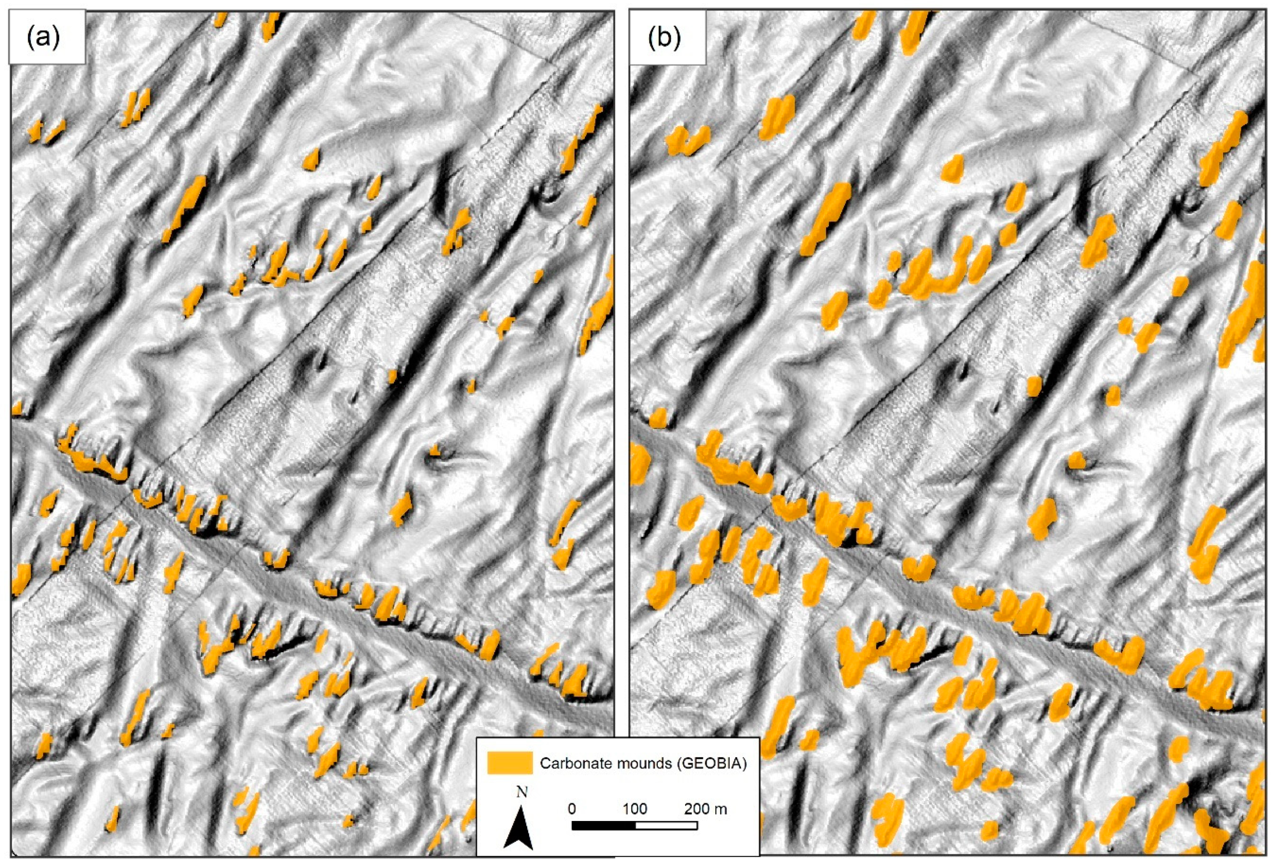
- Buffering polygons: A 5-m buffer was applied around the classified polygons with the aim to include the lower parts of carbonate mounds. The size of the buffer was selected after trials and visual assessment of the results (Figure 7).
2.5. Reference Data and Accuracy Assessment
2.5.1. Sampling Design
2.5.2. Response Design
2.5.3. Analysis
3. Results
3.1. Reference Data
3.2. Map Accuracy
3.3. Spatial Comparison
4. Discussion
5. Conclusions
Author Contributions
Funding
Acknowledgments
Conflicts of Interest
References
- Roberts, J.M.; Wheeler, A.J.; Freiwald, A. Reefs of the Deep: The Biology and Geology of Cold-Water Coral Ecosystems. Science 2006, 312, 543–547. [Google Scholar] [CrossRef] [PubMed]
- Bongiorni, L.; Mea, M.; Gambi, C.; Pusceddu, A.; Taviani, M.; Danovaro, R. Deep-water scleractinian corals promote higher biodiversity in deep-sea meiofaunal assemblages along continental margins. Biol. Conserv. 2010, 143, 1687–1700. [Google Scholar]
- Baillon, S.; Hamel, J.F.; Wareham, V.E.; Mercier, A. Deep cold-water corals as nurseries for fish larvae. Front. Ecol. Environ. 2012, 10, 351–356. [Google Scholar] [CrossRef]
- Söffker, M.; Sloman, K.A.; Hall-Spencer, J.M. In situ observations of fish associated with coral reefs off Ireland. Deep. Res. Part I Oceanogr. Res. Pap. 2011, 58, 818–825. [Google Scholar] [CrossRef]
- Costello, M.J.; McCrea, M.; Freiwald, A.; Lundälv, T.; Jonsson, L.; Bett, B.J.; van Weering, T.C.E.; de Haas, H.; Roberts, J.M.; Allen, D. Role of cold-water Lophelia pertusa coral reefs as fish habitat in the NE Atlantic. In Cold-Water Corals and Ecosystems; Springer: Berlin, Heidelberg, 2005; pp. 771–805. [Google Scholar]
- Hoegh-Guldberg, O.; Poloczanska, E.S.; Skirving, W.; Dove, S. Coral Reef Ecosystems under Climate Change and Ocean Acidification. Front. Mar. Sci. 2017, 4. [Google Scholar] [CrossRef]
- Titschack, J.; Baum, D.; De Pol-Holz, R.; López Correa, M.; Forster, N.; Flögel, S.; Hebbeln, D.; Freiwald, A. Aggradation and carbonate accumulation of Holocene Norwegian cold-water coral reefs. Sedimentology 2015, 62, 1873–1898. [Google Scholar] [CrossRef]
- Lindberg, B.; Mienert, J. Postglacial carbonate production by cold-water corals on the Norwegian Shelf and their role in the global carbonate budget. Geology 2005, 33, 537–540. [Google Scholar] [CrossRef]
- Althaus, F.; Williams, A.; Schlacher, T.; Kloser, R.J.; Green, M.; Barker, B.; Bax, N.; Brodie, P. Impacts of bottom trawling on deep-coral ecosystems of seamounts are long-lasting. Mar. Ecol. Prog. Ser. 2009, 397, 279–294. [Google Scholar] [CrossRef]
- Hall–Spencer, J.; Allain, V.; Fosså, J.H. Trawling damage to Northeast Atlantic ancient coral reefs. Proc. R. Soc. London. Ser. B Biol. Sci. 2002, 269, 507–511. [Google Scholar] [CrossRef]
- Fosså, J.H.; Mortensen, P.B.; Furevik, D.M. The deep-water coral Lophelia pertusa in Norwegian waters: Distribution and fishery impacts. Hydrobiologia 2002, 471, 1–12. [Google Scholar] [CrossRef]
- Roberts, J.M.; Cairns, S.D. Cold-water corals in a changing ocean. Curr. Opin. Environ. Sustain. 2014, 7, 118–126. [Google Scholar] [CrossRef]
- Fisher, C.R.; Hsing, P.-Y.; Kaiser, C.L.; Yoerger, D.R.; Roberts, H.H.; Shedd, W.W.; Cordes, E.E.; Shank, T.M.; Berlet, S.P.; Saunders, M.G.; Larcom, E.A.; Brooks, J.M. Footprint of Deepwater Horizon blowout impact to deep-water coral communities. Proc. Natl. Acad. Sci. 2014, 111, 11744–11749. [Google Scholar] [CrossRef] [PubMed]
- Torrents, O.; Tambutté, E.; Caminiti, N.; Garrabou, J. Upper thermal thresholds of shallow vs. deep populations of the precious Mediterranean red coral Corallium rubrum (L.): Assessing the potential effects of warming in the NW Mediterranean. J. Exp. Mar. Bio. Ecol. 2008, 357, 7–19. [Google Scholar] [CrossRef]
- Guinotte, J.M.; Orr, J.; Cairns, S.; Freiwald, A.; Morgan, L.; George, R. Will human-induced changes in seawater chemistry alter the distribution of deep-sea scleractinian corals? Front. Ecol. Environ. 2006, 4, 141–146. [Google Scholar] [CrossRef]
- Dullo, W.-C.; Flögel, S.; Rüggeberg, A. Cold-water coral growth in relation to the hydrography of the Celtic and Nordic European continental margin. Mar. Ecol. Prog. Ser. 2008, 371, 165–176. [Google Scholar] [CrossRef]
- Kiriakoulakis, K.; Freiwald, A.; Fisher, E.; Wolff, G.A. Organic matter quality and supply to deep-water coral/mound systems of the NW European Continental Margin. Int. J. Earth Sci. 2007, 96, 159–170. [Google Scholar] [CrossRef]
- Edinger, E.N.; Sherwood, O.A.; Piper, D.J.W.; Wareham, V.E.; Baker, K.D.; Gilkinson, K.D.; Scott, D.B. Geological features supporting deep-sea coral habitat in Atlantic Canada. Cont. Shelf Res. 2011, 31, 69–84. [Google Scholar] [CrossRef]
- Thorsnes, T.; Bellec, V.K.; Dolan, M.F.J. Cold-water coral reefs and glacial landforms from Sula Reef, mid-Norwegian shelf. Geol. Soc. London, Mem. 2016, 46, 307–308. [Google Scholar] [CrossRef]
- Buhl-Mortensen, L.; Vanreusel, A.; Gooday, A.J.; Levin, L.A.; Priede, I.G.; Buhl-Mortensen, P.; Gheerardyn, H.; King, N.J.; Raes, M. Biological structures as a source of habitat heterogeneity and biodiversity on the deep ocean margins. Mar. Ecol. 2010, 31, 21–50. [Google Scholar] [CrossRef]
- Freiwald, A.; Rogers, A.; Hall-Spencer, J.; Guinotte, J.; Davies, A.; Yesson, C.; Martin, C.; Weatherdon, L. Global distribution of cold-water corals (version 5.0). Fifth update to the dataset in Freiwald et al. (2004) by UNEP-WCMC, in collaboration with Andre Freiwald and John Guinotte.
- Anderson, O.F.; Guinotte, J.M.; Rowden, A.A.; Clark, M.R.; Mormede, S.; Davies, A.J.; Bowden, D.A. Field validation of habitat suitability models for vulnerable marine ecosystems in the South Pacific Ocean: Implications for the use of broad-scale models in fisheries management. Ocean Coast. Manag. 2016, 120, 110–126. [Google Scholar] [CrossRef]
- Wheeler, A.J.; Beyer, A.; Freiwald, A.; de Haas, H.; Huvenne, V.A.I.; Kozachenko, M.; Olu-Le Roy, K.; Opderbecke, J. Morphology and environment of cold-water coral carbonate mounds on the NW European margin. Int. J. Earth Sci. 2007, 96, 37–56. [Google Scholar] [CrossRef]
- De Clippele, L.H.; Gafeira, J.; Robert, K.; Hennige, S.; Lavaleye, M.S.; Duineveld, G.C.A.; Huvenne, V.A.I.; Roberts, J.M. Using novel acoustic and visual mapping tools to predict the small-scale spatial distribution of live biogenic reef framework in cold-water coral habitats. Coral Reefs 2017, 36, 255–268. [Google Scholar] [CrossRef]
- Diesing, M.; Thorsnes, T. Mapping of Cold-Water Coral Carbonate Mounds Based on Geomorphometric Features: An Object-Based Approach. Geosciences 2018, 8, 34. [Google Scholar] [CrossRef]
- Bellec, V.K.; Thorsnes, T.; Bøe, R. Mapping of bioclastic sediments - data, methods and confidence. NGU-rapport 2014, 2014.006, 23. [Google Scholar]
- Freiwald, A.; Hühnerbach, V.; Lindberg, B.; Wilson, J.B.; Campbell, J. The Sula Reef Complex, Norwegian shelf. Facies 2002, 47, 179–200. [Google Scholar] [CrossRef]
- Bellec, V.K.; Bøe, R.; Rise, L.; Lepland, A.; Thorsnes, T.; Bjarnadóttir, L.R. Seabed sediments (grain size) of Nordland VI, offshore north Norway. J. Maps 2017, 13, 608–620. [Google Scholar] [CrossRef]
- Wright, D.J.; Pendleton, M.; Boulware, J.; Walbridge, S.; Gerlt, B.; Eslinger, D.; Sampson, D.H.E. Unified Geomorphological Analysis Workflows with Benthic Terrain Modeler. Geosciences 2018, 8, 94. [Google Scholar] [CrossRef]
- Li, J.; Heap, A.D.; Potter, A.; Huang, Z.; Daniell, J.J. Can we improve the spatial predictions of seabed sediments? A case study of spatial interpolation of mud content across the southwest Australian margin. Cont. Shelf Res. 2011, 31, 1365–1376. [Google Scholar] [CrossRef]
- Huang, Z.; Siwabessy, J.; Nichol, S.; Anderson, T.; Brooke, B. Predictive mapping of seabed cover types using angular response curves of multibeam backscatter data: Testing different feature analysis approaches. Cont. Shelf Res. 2013, 61–62, 12–22. [Google Scholar] [CrossRef]
- eCognition eCognition Developer 9. Available online: http://www.ecognition.com/suite/ecognition-developer (accessed on 10 May 2018).
- Wilson, M.F.J.; O’Connell, B.; Brown, C.; Guinan, J.C.; Grehan, A.J. Multiscale terrain analysis of multibeam bathymetry data for habitat mapping on the continental slope. Mar. Geod. 2007, 30, 3–35. [Google Scholar]
- Lundblad, E.R.; Wright, D.J.; Miller, J.; Larkin, E.M.; Rinehart, R.; Naar, D.F.; Donahue, B.T.; Anderson, S.M.; Battista, T. A Benthic Terrain Classification Scheme for American Samoa. Mar. Geod. 2006, 29, 89–111. [Google Scholar] [CrossRef]
- ArcGIS Pro Overview of georeferencing. Available online: http://pro.arcgis.com/en/pro-app/help/data/imagery/overview-of-georeferencing.htm (accessed on 27 September 2018).
- Jakobsson, M.; Gyllencreutz, R.; Mayer, L.A.; Dowdeswell, J.A.; Canals, M.; Todd, B.J.; Dowdeswell, E.K.; Hogan, K.A.; Larter, R.D. Mapping submarine glacial landforms using acoustic methods. Geol. Soc. London, Mem. 2016, 46, 17–40. [Google Scholar] [CrossRef]
- Blaschke, T.; Hay, G.J.; Kelly, M.; Lang, S.; Hofmann, P.; Addink, E.; Queiroz Feitosa, R.; van der Meer, F.; van der Werff, H.; van Coillie, F.; Tiede, D. Geographic Object-Based Image Analysis—Towards a new paradigm. ISPRS J. Photogramm. Remote Sens. 2014, 87, 180–191. [Google Scholar] [CrossRef] [PubMed]
- Hay, G.J.; Castilla, G. Geographic Object-Based Image Analysis (GEOBIA): A new name for a new discipline. In Object-Based Image Analysis: Spatial Concepts for Knowledge-Driven Remote Sensing Applications; Blaschke, T., Lang, S., Hay, G.J., Eds.; Springer: Berlin, Germany, 2008; pp. 75–89. [Google Scholar]
- Schiewe, J. Segmentation of high-resolution remotely sensed data—Concepts, applications and problems. In Proceedings of the Symposium on Geospatial theory, Processing and Applications, Ottawa, ON, Canada, 9–12 July 2002. [Google Scholar]
- Olofsson, P.; Foody, G.M.; Herold, M.; Stehman, S.V.; Woodcock, C.E.; Wulder, M.A. Good practices for estimating area and assessing accuracy of land change. Remote Sens. Environ. 2014, 148, 42–57. [Google Scholar] [CrossRef]
- Stehman, S.V.; Czaplewski, R.L. Design and Analysis for Thematic Map Accuracy Assessment—An application of satellite imagery. Remote Sens. Environ. 1998, 64, 331–344. [Google Scholar] [CrossRef]
- Cochran, W.G. Sampling techniques, 3rd ed.; John Wiley & Sons: New York, NY, USA, 1977. [Google Scholar]
- Kuhn, M. Building Predictive Models in R Using the caret Package. J. Stat. Software 2008, 28, 1–26. [Google Scholar] [CrossRef]
- Foody, G.M. Thematic Map Comparison: Evaluating the Statistical Significance of Differences in Classification Accuracy. Photogramm. Eng. Remote Sens. 2004, 70, 627–633. [Google Scholar] [CrossRef]
- Mitchell, P.J.; Downie, A.-L.; Diesing, M. How good is my map? A tool for semi-automated thematic mapping and spatially explicit confidence assessment. Environ. Model. Softw. 2018, 108, 111–122. [Google Scholar] [CrossRef]
- Rattray, A.J.; Ierodiaconou, D.; Monk, J.; Laurenson, L.; Kennedy, P. Quantification of Spatial and Thematic Uncertainty in the Application of Underwater Video for Benthic Habitat Mapping. Mar. Geod. 2014, 37, 315–336. [Google Scholar] [CrossRef]
- Fielding, A.H.; Bell, J.F. A review of methods for the assessment of prediction errors in conservation presence/absence models. Environ. Conserv. 1997, 24, 38–49. [Google Scholar] [CrossRef]
- Lyons, M.B.; Keith, D.A.; Phinn, S.R.; Mason, T.J.; Elith, J. A comparison of resampling methods for remote sensing classification and accuracy assessment. Remote Sens. Environ. 2018, 208, 145–153. [Google Scholar] [CrossRef]


| Derivative | Description | Reference |
|---|---|---|
| Slope [°] | The maximum slope gradient. | [33] |
| Curvature | The rate of change of slope. | [33] |
| Profile and plan curvature | Profile curvature is measured parallel to the slope, plan curvature perpendicular. | [33] |
| Bathymetric positioning index (BPI) [m] | Vertical position of a cell relative to its neighborhood. | [34] |
| Surface area to Planar area * | Computes a ratio between the three-dimensional surface area and the planar area of the surface. | [29] |
| Second order polynomial transformation * | Creates bend or curved adjusted transformation of the dataset | [35] |
| Observed Absence | Observed Presence | |
|---|---|---|
| Predicted absence | True negative (TN) | False negative (FN) |
| Predicted presence | False positive (FP) | True positive (TP) |
| No. of Observations | Fraction | Meaning | |
|---|---|---|---|
| Presence | 73 | 0.241 | = Prevalence |
| Absence | 230 | 0.759 | = No-information Rate |
| Sum | 303 | 1 |
| Manual | Terrain Analysis | GEOBIA | ||||
|---|---|---|---|---|---|---|
| OA | OP | OA | OP | OA | OP | |
| PA | 221 | 18 | 211 | 14 | 221 | 26 |
| PP | 9 | 55 | 19 | 59 | 9 | 47 |
| PCC | 0.9109 | 0.8911 | 0.8845 | |||
| 95% CI | (0.873, 0.9405) | (0.8505, 0.9238) | (0.843, 0.9182) | |||
| NIR | 0.7591 | 0.7591 | 0.7591 | |||
| P-Value [Acc > NIR] | 7.40E-12 | 4.44E-09 | 2.85E-08 | |||
| Sensitivity | 0.7534 | 0.8082 | 0.6438 | |||
| Specificity | 0.9609 | 0.9174 | 0.9609 | |||
| p-values\χ2 | Manual | Terrain Analysis | GEOBIA |
|---|---|---|---|
| manual | - | 0.521 | 1.225 |
| terrain analysis | 0.471 | - | 0.025 |
| GEOBIA | 0.268 | 0.874 | - |
| Manual | Terrain Analysis | GEOBIA | |
|---|---|---|---|
| Number of polygons | 3559 | 3247 | 4866 |
| Area (km2) | 6.01 | 7.35 | 5.01 |
| Method | Manual | Terrain Analysis | GEOBIA |
|---|---|---|---|
| Has highest | specificity | sensitivity | specificity |
| Minimizes | number of false positives | number of false negatives | number of false positives |
| Best predicts | Absence of mounds | Presence of mounds | Absence of mounds |
© 2019 by the authors. Licensee MDPI, Basel, Switzerland. This article is an open access article distributed under the terms and conditions of the Creative Commons Attribution (CC BY) license (http://creativecommons.org/licenses/by/4.0/).
Share and Cite
Jarna, A.; Baeten, N.J.; Elvenes, S.; Bellec, V.K.; Thorsnes, T.; Diesing, M. Semi-Automatic Versus Manual Mapping of Cold-Water Coral Carbonate Mounds Located Offshore Norway. ISPRS Int. J. Geo-Inf. 2019, 8, 40. https://doi.org/10.3390/ijgi8010040
Jarna A, Baeten NJ, Elvenes S, Bellec VK, Thorsnes T, Diesing M. Semi-Automatic Versus Manual Mapping of Cold-Water Coral Carbonate Mounds Located Offshore Norway. ISPRS International Journal of Geo-Information. 2019; 8(1):40. https://doi.org/10.3390/ijgi8010040
Chicago/Turabian StyleJarna, Alexandra, Nicole J. Baeten, Sigrid Elvenes, Valérie K. Bellec, Terje Thorsnes, and Markus Diesing. 2019. "Semi-Automatic Versus Manual Mapping of Cold-Water Coral Carbonate Mounds Located Offshore Norway" ISPRS International Journal of Geo-Information 8, no. 1: 40. https://doi.org/10.3390/ijgi8010040
APA StyleJarna, A., Baeten, N. J., Elvenes, S., Bellec, V. K., Thorsnes, T., & Diesing, M. (2019). Semi-Automatic Versus Manual Mapping of Cold-Water Coral Carbonate Mounds Located Offshore Norway. ISPRS International Journal of Geo-Information, 8(1), 40. https://doi.org/10.3390/ijgi8010040