Abstract
Understanding the complex hydrodynamics and transport processes are of primary importance to alleviate and control the eutrophication problem in lakes. Numerical models are used to simulate these processes. However, it is often difficult to perform such a numerical modeling simulation for common users. This study presented an integrated graphic modeling system designed for three-dimensional hydrodynamic and water quality simulation in lakes. The system, called the Lake Modeling System (LMS), provides necessary functionalities streamlined for hydrodynamic modeling. The LMS provides a geographic information system (GIS)-based data processing framework to establish a model and provides capabilities for displaying model input and output information. The LMS also provides mapping and visualization tools to support the model development process. All of these features in a GIS-based framework makes the task of complex hydrodynamic and water quality modeling easier. The applicability of the LMS is demonstrated by a case study in Lake Donghu, which is a large urban lake in the middle reaches of the Yangtze River in China. The LMS was utilized to setup and calibrate a model for Lake Donghu. Then the model was used to study the effects of a water diversion project on the change in hydrodynamics and the water quality.
1. Introduction
Lakes are valuable natural resources for water supply, food, irrigation, transportation, recreation, and hydropower. Due to near-lake development, lake ecosystems are being threatened by anthropogenic impacts, including nutrient pollution, increasing populations and intensification of land use. Eutrophication of water bodies, one of the most widespread environmental problems, is found worldwide, from the Great Lakes of North America [1] to Lake Tai of China [2] and Lake Victoria in Africa [3]. Understanding the complex hydrodynamics and transport processes are of primary importance to alleviate and control the eutrophication problem in lakes.
Hydrodynamics is highly variable among lakes due to the different geometries, surrounding topographies, hydrological loadings, and meteorological conditions. Hydrodynamics and transport processes in lakes are also inherently three-dimensional (3D), driven by interactions of wind, surface thermodynamics, and topography. The numerical model has become one of the most powerful tools for studying these complex dynamics. Such models can help us to know more clearly what exactly is behind the water quality changes and eutrophication and help lake managers select optimal control strategies. In past decades, many models and commercial software have been developed, including Finite Volume Coastal Ocean Model (FVCOM) [4], Princeton Ocean Model (POM) [5], Delft3D [6], Environmental Fluid Dynamics Code (EFDC) [7], and MIKE3 [8]. These models were initially developed for ocean modeling; nevertheless they have been widely used to study a variety of lake water issues, including lake water resources management [9], seasonal circulation, thermal structure [10,11], and harmful algal blooms [12,13].
Despite the fact that numerical models and scientific data sets are available for lakes’ numerical modeling, great challenges remain for end users to conduct such modeling. On the one hand, a variety of datasets are required to setup and calibrate a model, including bathymetry, meteorological data, observations of hydrological variables (e.g., streamflow, water level, evaporation, etc.), water quality variables (e.g., dissolved oxygen, chlorophyll, etc.), and many others. These data are usually large in volume, multisource, multivariable, multidimensional, and heterogeneous, with complex spatial and temporal regimes. Thus, incorporating all the data in the modeling process and interpreting the results during decision making requires intensive data processing efforts and a comprehensive understanding of the model. On the other hand, the setup of a numerical model involves many steps, including computational grid generation, initial and open boundary condition settings, model calibration, simulation and results analysis. It is often difficult to perform such a numerical modeling simulation, even for a skilled user. These challenges have seriously hindered the wider application of numerical models in scientific research and management practice. Therefore, a comprehensive system that can handle the entire procedure of lake hydrodynamic and water quality modeling, from data preparation at the very beginning to analysis and visualization of model outputs at the end, is highly desired.
It has been widely recognized that the Geographic Information System (GIS) plays a central role in developing such a modeling system. Many efforts have been made to integrate the GIS with numerical models for surface water (rivers, lakes, surface hydrology), coastal and ocean modeling. For example, Liang et al. developed an automatic numerical simulation program for coastal waters by integrating FVCOM with a GIS [14]; Ng et al. integrated a GIS with a complex three-dimensional hydrodynamic sediment and heavy metal transport numerical model and applied the integrated system to the Pearl River Estuary in China [15]; Qin and Lin developed a system for costal seiches monitoring and forecasting by integrating FVCOM into a web-GIS based framework [16]. Such integrations not only benefit the preprocessing and postprocessing procedures of the modeling but also provide the system with spatial data analysis and visualization capabilities. However, there are several weaknesses associated with the existing systems, especially for lake modeling. First, many GIS-hydrodynamic water quality models are two-dimensional. Since hydrodynamics in lakes is intrinsically three-dimensional, such models may oversimplify the actual situations and produce results with limited accuracy. Second, popular GIS platforms, such as ArcGIS Map and Google Earth, are often used as the GIS environment by existing systems. However, these platforms are not specifically designed for hydrodynamic studies and cannot easily handle the diversified data types involved in the hydrodynamic modeling, especially time series data [17].
In this paper, we present the design and development of the Lake Modeling System (LMS), which is a modeling system for three-dimensional (3D) hydrodynamic and water quality model. LMS provides graphic user interface (GUI) for end users to build 3D model. It provides a GIS-based data processing framework for establishing the model and provides capabilities for displaying and modifying model elements (model grids) and boundary conditions. The interface of LMS is two-dimensional (2D) but allows to display and analyze model inputs and outputs that are multi-dimensional. All of these features will make the task of hydrodynamic and water quality modeling easier. The applicability of LMS is illustrated by a case study in Lake Donghu, which is a large urban lake in the middle reaches of the Yangtze River.
In the remainder of this paper, Section 2 introduces the framework of the LMS, including the system design and implementation. The details of setting up and running the model using the LMS are also illustrated. Section 3 describes the application case of the LMS in the Lake Donghu in China. The results and analysis of the Lake Donghu model are presented in Section 4, and conclusions are provided in Section 5.
2. Framework of the System
2.1. Introduction to FVCOM-LAKE
The current version of the LMS has been made compatible with the Finite Volume Coastal Ocean Model (FVCOM) [4]. FVCOM appears to be one of the most popular modules for near shore numerical simulation based on its prevalence in simulation literature [18,19]. It is an unstructured-grid, finite-volume, three-dimensional (3-D) primitive equation ocean model with a generalized, terrain-following coordinate system in the vertical and a triangular grid in the horizontal. The unstructured grid can be designed to provide a customized variable resolution to both lake boundaries and bathymetry.
FVCOM uses the coordinate, which enables for a smooth representation of irregular bottom topography to be obtained. The coordinate transformation is defined as:
where H is the bottom depth (relative to ) and is the height of the free surface (relative to ); is the total water column depth; and varies from −1 at the bottom to 0 at the surface. In this coordinate, the governing equations of FVCOM consist of the following continuity, momentum, temperature, salinity and density equations:
where are the velocity components, respectively; is the temperature; is the salinity; is the density; is the Coriolis parameter; is the gravitational acceleration; is the vertical eddy viscosity coefficient; and is the thermal vertical eddy diffusion coefficient. represent the horizontal momentum, thermal, and salt diffusion terms, respectively. and are parameterized using the modified Mellor and Yamada level-2.5 (MY-2.5) turbulent closure scheme [20,21,22]. FVCOM is numerically solved using a split-mode method.
The water quality model used in this study is the Water Analysis Simulation Program (WASP) [23]. The conceptual model framework is shown in Figure 1. The model contains eight state variables, including dissolved oxygen (DO; mg O2 L−1), carbonaceous biochemical oxygen demand (CBOD; mg O2 L−1), nitrite nitrogen (NO3; mg N L−1), ammonium nitrogen (NH4; mg N L−1), organic nitrogen (ON; mg N L−1), organic phosphorus (OP; mg P L−1), soluble reactive phosphorus (PO4; mg P L−1), and phytoplankton biomass expressed as chlorophyll (CHL; μg Chl α L−1). The governing equations of the WASP are described in detail in [24]. The WASP was coupled with FVCOM and can be run in an online mode. In this study, the sum of NH4, NO3, and ON is regarded as the total nitrogen (TN), and the sum of OP and PO4 is regarded as the total phosphorus (TP).
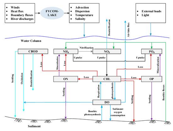
Figure 1.
Conceptual framework of the WASP water quality model.
The preferred environment for building and running FVCOM is Linux. However, LMS is designed to run on Windows. To this end, the source code of FVCOM was ported to the Windows environment and was compiled as a standalone execution program using the Intel Fortran compiler. This modified version of FVCOM was called FVCOM-LAKE. The original algorithm of FVCOM has not been modified.
2.2. System Design
Figure 2 presents a conceptual design of the GIS-model integration framework. The framework is composed of four major parts: the GIS-based user interface (UI), shared libraries, the three-dimensional hydrodynamic and water quality model (i.e., FVCOM-LAKE) and data sources. The user interface provides common GIS capabilities, such as mapping, management and analysis of spatial information, and provides geo-processing tools. The UI also enables to create a model and perform model processing such as visualization of model inputs/outputs and animation of results. The data and GIS libraries provides shared functions for reading, querying and manipulating data from the underlying data sources. The model wrapper provides functions that enable the system to communicate with the numerical model through input/output files. The actual execution of the numerical model is a stand-alone program that does not require any GIS capabilities. The data sources include GIS data files (i.e., raster and vector files), the relation database that stores time series, and model input/output files.
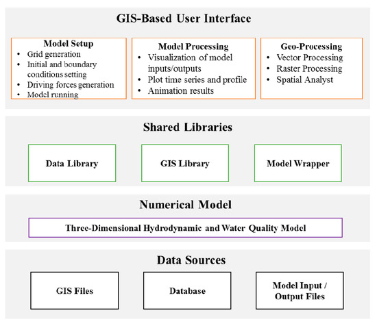
Figure 2.
Conceptual diagram of integration of a GIS and a three-dimensional hydrodynamic and water quality model.
2.3. System Implimentation
2.3.1. System Overview
LMS was developed using C# language based on Microsoft .NET platform. The DotSaptial library [25] was employed for providing GIS environment. DotSpatial is a free and open source GIS library written for .NET. It allows developers to incorporate spatial data, analysis and mapping functionality into their applications. The graphic user interface of LMS is shown in Figure 3a. LMS has a familiar interface similar to most desktop GIS applications. The main window contains a main menu, a map viewer, a legend, a toolbox and toolbars. The map view is the main visualization element. LMS provides common functionalities to display and manage geospatial data, such as zoom, pan, query, symbology, conversion, and many other. The toolbox also provides a set of tools to perform fundamental GIS operations. LMS supports common vector and raster geospatial data file formats. The vector data format supported is shapefile, and the raster data formats supported include TIF, PNG, JPEG, and others. LMS uses the project to organize the model information and other resources required for the modeling. When opening a project, the model structure is presented in the project manager (Figure 3b).
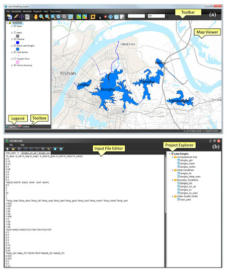
Figure 3.
Main graphic user interface of LMS: (a) Map Viewer; and (b) Project Manager.
2.3.2. Grid Generation
LMS provides a grid generation tool to produce a high-quality triangular grid. This tool is based on the Delaunay triangulation algorithm developed by Shewchuk [26]. Figure 4 presents the grid generation tool. The first step of using the tool is to specify a shapefile that represents a lake boundary. To improve the grid’s quality, the boundary line must be preprocessed, which includes smoothing and redistributing the line’s vertices. The LMS provides a tool to perform these preprocessing operations. The next step is to select a raster file that represents the lake’s bathymetry. Then, users can specify the parameters that control the size and number of triangular elements and the method of interpolating the bathymetry. At this point, all requirements for the generation are satisfied, and the grid can be automatically generated with the user’s click of a button. During the generation, bathymetry data will be automatically interpolated to each node of the grid. LMS also accepts a grid file format generated by other software, such as the Aquaveo Surface-water Modeling System.
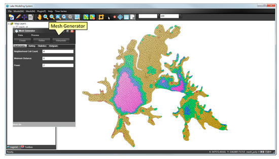
Figure 4.
Grid generation tool.
The generated grid is represented by two shapefiles: one is a polygon shapefile that represents the triangular elements of the grid, and the other is a point shapefile that represents the nodes of the grid. These two shapefiles will be added to the map view after the generation. The grid input files required by FVCOM-LAKE will also be generated.
2.3.3. Initial and Boundary Conditions Settings
Users must define initial hydrodynamic values and initial quality state variables at each node of the grid. The state variables include the water level, water temperature and salinity, and the eight water column state variables. Ideally, the initial values should be determined based on observations. If such observations are unavailable, the initial values could be simply set as constants. If there are sufficient observations, the initial values could be assigned to the grid using several GIS tools provided by LMS. For example, if observations are made on point stations, the Interpolation Tool could be used to interpolate the observed point values to each node of the grid. Sometimes results generated by other models or products produced by remote sensing methods (e.g., MODIS products) could also be used to set the initial values. These results or products are usually archived using the NetCDF format or other popular raster formats (e.g., TIF). The LMS enables initial conditions to be set by extracting the values from these data sets to the grid. Figure 5 presents the interface used to set the river boundary condition. The user can specify nodes where river inflow/outflow would be applied, and set the discharge and water temperature at the nodes.
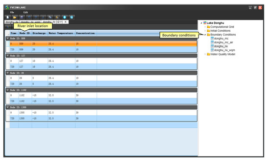
Figure 5.
Interface used to set river boundary condition.
2.3.4. Driving Force and Calibration Dataset Generation
FVCOM-LAKE requires hourly meteorological data as the driving force. The meteorological variables include precipitation, air pressure, temperature, wind speed and direction, relative humidity, and sunshine hours. The heat-fluxes at the water surface, including the sensible heat flux, the latent flux, the incoming longwave flux, the outgoing longwave flux and the incident short wave flux are automatically calculated based on the meteorological data. The meteorological data are often archived in various formats, such as NetCDF, TXT, and Excel. LMS provides a set of conversion tools to convert these different formats into the input file required by FVCOM-LAKE. The other driving forces include water discharge and containment concentration at rivers or drainage facilities. Observations made at sites or stations, such as the water level, water temperature and water quality concentrations, are usually used to conduct model calibration. The LMS uses database to store these observations. The user can use ODM Database Manager to import and manage the calibration datasets.
2.3.5. Modeling Running and Postprocessing
The users can start a model run once all necessary input files are ready. The running information (e.g., simulation time, execution time, etc.) is synchronously displayed in a window. Any warnings or errors information encountered during the modeling simulation will also be displayed in the window. The users can stop the simulation at any time. The LMS allows the users to analyze the model outputs at any time before the simulation is finished. When a model simulation takes long time to finish (e.g., hours or even days), this functionality is very useful since it allows the user to investigate problems or errors and start a new simulation immediately.
The output of the FVCOM-LAKE model consists of a set of binary files. The key output variables include horizontal velocity magnitude and direction, vertical velocity magnitude, water level, and concentration of water quality variables. With some simple operations, modeling results can be directly loaded from the output files, processed and then displayed in the GIS environment. In LMS, each model entity (e.g., grid, river inlet/outlets and boundaries) is represented by a FeatureSet object, which is a general object in most existing GIS libraries. The FeatureSet object is used a shared data model between GIS and the system. The loaded data is visualized through the FeatureSet object. In addition, LMS provides several tools to display the modeling results in the form of time series, and profile.
The profile tool extracts values at a selected point from each of the depth layers and then create a profile plot using the extracted values. When using the profile tool, the user can click any point within the modeling domain. The time series tool is used to display the time series of a selected variable associated with a given point selected in a modeling domain. As the lake’s hydrodynamics is continuously changing, the dynamic display of the modeling results is essential for examining and analyzing spatiotemporal variations of the lake data. The LMS provides an animation tool that enables the model outputs to be animated for the selected time span. Users are able to manipulate the animation through a controller which provides common operations, including play, stop, pause, forward, and backward. As the output data are loaded onto the computer memory, the system can provide fluent animation. In addition, the system is able to perform basic data analyses (e.g., deriving mean, sum, and maximum and minimum values) for user-specified time periods and spatial chart view. This functionality is very useful in examining modeling results.
3. Case Study
3.1. Study Area
An example is presented in this section to illustrate the use of the LMS for setting up a new model run. Lake Donghu, a large urban lake, was selected as the case study area (Figure 6a). The lake is fully located within the urban area of Wuhan city. It covers an area of 30.7 km2 and has an average depth of 2.2 m. There are other five urban lakes around Lake Donghu, including Lakes Shahu, Beihu, Yandonghu, and Yanxihu. Lake Donghu used to connect with Yangtze River. However, the lake was completely separated from the Yangtze River in the 1980s and was divided into a set of bays by roads. As presented in Figure 6b, the major bays include Tanglinhu, Shaojihu, Guozheng, Tuanhu, Miaohu, Yujiahu, Yingwohu, and Shuiguo Bays.
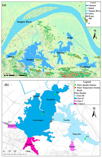
Figure 6.
The study area: (a) Lake Donghu and its surrounding urban lakes; and (b) water quality in Lake Donghu in May 2011.
Lake Donghu is a typical shallow lake with limited contamination purification capabilities. Pollutants are difficult to remove once they enter the lake. Before the 1950s, the lake was in good health, and lake water could be used as drinking water. In the 1960s, the lake underwent oligotrophic conditions, which gradually became mesotrophic by 1981. Since then, the situation has worsened due to increasing contamination factors, such as increasing amounts of aquaculture, rapid urbanization, and large quantities of wastewater discharged into the lake without proper treatment.
Monthly samples of DO, nutrients and chlorophyll were collected at Stations W1 to W4 (Figure 6) by the Water Authority of Wuhan. Based on the measurements made in May 2011, the water quality classification in the major bays of Lake Donghu was determined according to the Chinese national water quality standard [27] and presented in Figure 6b. It can be seen that water qualities in most bays are worse than Class III. According to the target of water quality improvement, the water quality in Lake Donghu must meet the Class III standard.
In addition to Lake Donghu, the other urban lakes shown in Figure 6a also have serious eutrophication problems. To improve the water quality of the lake groups, the Wuhan Municipal Government lunched a water diversion project. The project was intended to dilute and flush the nutrient concentrations from the lakes and decrease the residence time (or self-purification rates) by diverting water from the Yangtze River. Water diversion has been proven to be a successful strategy for improving water quality; it has been implemented in many Chinese lakes such as Taihu [28], Chaohu [29], and Dianchi [30]. Previous water diversion projects suggest that it is necessary and helpful to simulate hydrodynamic and water quality processes under different water diversion scenarios. This section illustrates how to use the LMS to setup a FVCOM-LAKE model for Lake Donghu. Then, the model was used to study the effects of water diversion on the change in hydrodynamics and improvement of the water quality under different water diversion scenarios.
3.2. Model Setup
To generate the computational grid, the bathymetry and lake boundary were collected. The bathymetry was obtained from a filed investigation conducted in 2006. The grid was generated using the LMS; it comprises 3476 nodes and 6067 triangular elements with approximate minimum and maximum element sides of 40 and 60 m, respectively. The maximum water depth was approximately 4.5 m, and the minimum depth was artificially set at 0.5 m at the lakeshore. Nodes were not allowed to be wet and dry. Depth levels were specified as sigma coordinates (terrain following) where the depth levels are equally spaced in the water column. The model has four sigma coordinate levels; each layer is 25% of the total water column depth. The bottom roughness was set to 0.0025 according to similar lakes.
The model simulation period ranged from 1 May 2011 to 31 July 2011. Data used to set the diving forces, boundary and initial conditions during the period were collected from different sources. Hourly meteorological data were obtained from a meteorological station near Lake Donghu. The original format of the meteorological data was an Excel file. LMS was used to transform the original data into a format acceptable by FVCOM-LAKE.
The initial water level and water temperature was set to 19.15 m and an isothermal temperature of 15 °C everywhere according to the observed values on March 1, 2011. The initial flow velocity was set at 0 m s−1. The initial values for the water quality state variables were specified separately for each bay based on observations (see Table 1). Investigations of pollution sources, including point sources and nonpoint sources in the lake area, were conducted in 2011. The nonpoint sources were generalized as point sources in the simulation. In total, seven major point-loadings entering the lake were specified. Based on the Courant–Friedrichs–Lewy (CFL) criterion, the internal mode time step of the integration was 300 s, while the external mode time step was 15 s.

Table 1.
Initial values of the water quality variables in the bays of Lake Donghu.
3.3. Model Calibration
Continuous observations of the water levels and water flow speed were unavailable for Lake Donghu, so alternatively daily averaged water temperatures measured at station T1 were used to calibrate the hydrodynamic model parameters. Monthly water quality observations made at stations W1-W5 were used to calibrate WASP model parameters.
The calibration was manually accomplished in a trial-and-error manner. For the hydrodynamic model, parameters related to the Mellor and Yamada turbulence model were set at the same values as the ones used in other hydrodynamic models. Similarly, the non-dimensionless viscosity parameter in the Smagorinsky formula was set to a constant value of 0.2. For the water quality model, the initial values of the parameters (Table 2) used in the WASP were specified based on published field studies performed on similar lakes and literature reviews, and previous WASP applications. Then, some of the key parameters were further tuned.
Table 2.
Parameter values used in the WASP water quality model.
3.4. Scenario Design
To investigate the influence of diversion from the Yangtze River to Lake Donghu, three diversion scenarios were designed (Table 3):
Table 3.
Water diversion scenarios.
- (1)
- The first scenario, named S1 (Figure 7a), has three inlets, P1, P2, and P3, and two outlets, P4 and P5. P1 and P2 divert water from the Yangtze river into Tanglin bay with inflows of 20 m3 s−1 and 10 m3 s−1, respectively; P3 diverts water from Lake Shahu into Shuiguo bay with an inflow of 5 m3 s−1; P4 drains water from Yingwo bay to Lake Yanxihu with an outflow of 20 m3 s−1; and P5 drains water from Guozheng bay to the Yangtze River with an outflow of 20 m3 s−1;
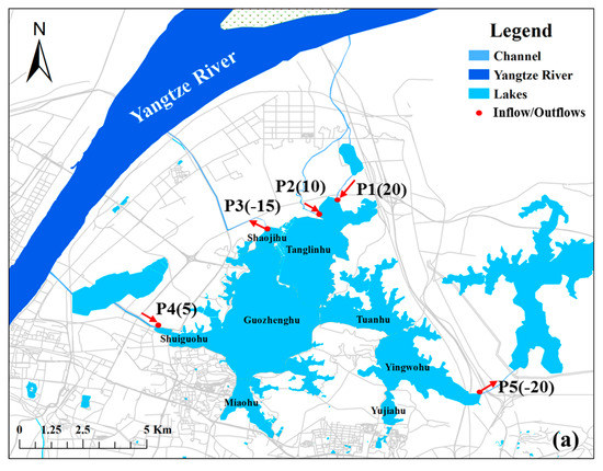
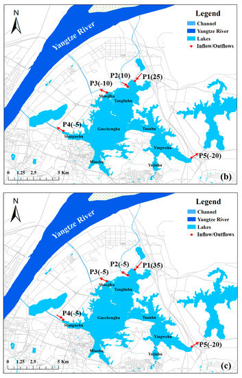 Figure 7. Water diversion scenario design: (a) scenario S1, (b) scenario S2, and (c) scenario S3. The values in brackets indicate discharge of inflow/outflow. The unit of the discharge is cubic meters per second. Positive values indicate inflows and negative values indicate outflows.
 - (2)
- The second scenario, named S2 (Figure 7b), has two inlets, P1 and P2, with inflows of 25 m3 s−1 and 10 m3 s−1, respectively, and three outlets, P3, P4 and P5, with outflows of 5 m3 s−1, 20 m3 s−1, and 10 m3 s−1, respectively;
- (3)
- The third scenario, named S3 (Figure 7c), only has one inlet, P3, with an inflow of 35 m3 s−1, and four outlets, P1, P2, P4 and P5, with outflows of 5 m3 s−1, 5 m3 s−1, 20 m3 s−1, and 5 m3 s−1, respectively.
The calibrated model was run to simulate each scenario for July 2011. All scenarios used the same driven forces and point loadings but different inflow/outflow boundary conditions. To make a comparison between scenarios, a set of indicators was designed (Table 4). These indicators could be grouped into two categories. The first category contains indicators that describe hydrodynamic characteristics, while the indicators in the second category describe improvements of water quality.
Table 4.
Indicators.
4. Results and Discussions
4.1. Calibration Results
Figure 8 shows a comparison of simulated and observed daily water temperature at location T1. The value of R2 indicates that the model adequately simulated a variation in the water temperature. The results of the simulated currents are visualized using the visualization tool of LMS (Figure 9). It can be seen that the model reproduced the main features of the wind-driven circulation in the lake quite well. The model calibration results of TN and TP for Stations W1, W2, W3, and W4 are shown in Figure 10 and Figure 11, respectively. In general, the model provided a reasonable reproduction of patterns and acceptable magnitudes for water quality constituents.
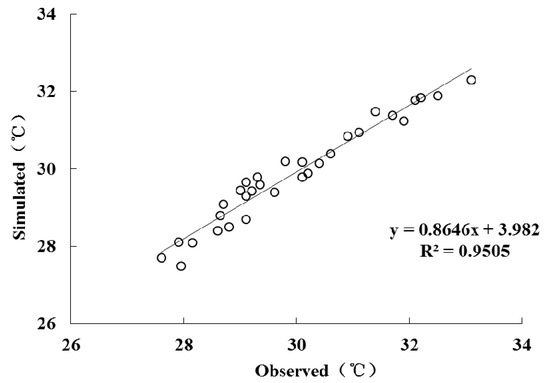
Figure 8.
Comparison of surface water temperature at Site T1.
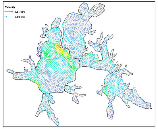
Figure 9.
Simulated depth-averaged circulation on 5 July 2011.
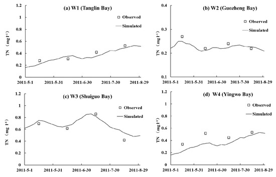
Figure 10.
Comparison of simulated and observed TN at four bays: (a) Tanglin Bay; (b) Guozheng Bay; (c) Shuiguo Bay; and (d) Yingwo Bay.
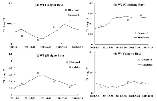
Figure 11.
Comparison of simulated and observed TP at four bays: (a) Tanglin Bay; (b) Guozheng Bay; (c) Shuiguo Bay; and (d) Yingwo Bay.
4.2. Scenario Analysis
4.2.1. Change of Lake Circulation Pattern
After implementing the water diversion project, hydrodynamic characteristics and circulation patterns would be dramatically changed. Figure 12 compares the circulation patterns of the three scenarios on the last day of the simulation period. For scenario S1 (Figure 12a), the movement of water develops in the entire lake area under the combined effects of water diversion at two inlets (P1, P2) and drainage at three outlets (P3, P4 and P5). The water diverted into the lake from P1 and P2 is moved southward and then divided into two branches: one branch is turned around and merges into the water diverted from P4, and then, the merged water continues to be moved northward and drained out of the lake from P3; the other branch is moved eastward and finally discharges at P5. Overall, water in the larges bays (e.g., Guozheng, Tanglin, Yingwo, and Shuiguo Bays) moves faster, while the water movement in the small lake branches is slow. It can also be seen that a local circulation is developed in the south part of the Guozheng bay, under the driving effect of the circulation, the water in Miao Bay flows northward. This circulation is beneficial to improving the water quality of the Miao Bay but also inevitably brings high-concentration pollutants in the Miao Bay into the main lake area.
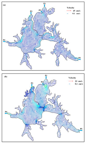
Figure 12.
Depth-averaged circulation on July 15, 2011 under scenarios S1 (a), S2 (b), and S3 (c).
In the second scenario S2 (Figure 12b), the freshwater is diverted from P1 and P2 flows through Tanglin Bay before being divided into two branches near the road: one branch is moved southeastward and finally discharged at P5; the other branch is turned around and then further divided into two subbranches, in which one subbranch is moved northward and discharged at P3, and the other subbranch is moved in an S path and is discharged at P4. Comparing scenarios S1 and S2, it can be determined that the circulation pattern is totally different in Guozheng Bay and Shuiguo Bay but is similar in Tanglin Bay and Yingwo Bay. Compared with that in scenario S1, the water flow in Guozheng bay under scenario S2 moves forward in a roundabout way, and the flow velocity is greatly affected, affecting the efficiency of water renewal.
Under scenario S3 (Figure 12c), the flow velocity in Shuiguo Bay is greatly accelerated by diverting freshwater from P4, then the diverted water moves northward and is divided into three branches: the first branch continues to move northward and is discharged at P3; the second branch also moves northward and is discharged at P1 and P2; and the third branch moves eastward and is discharged at P5.
Table 5 compares the hydrodynamic indicators under the three water diversion scenarios. Under scenarios S1, S2, and S3, average velocities are 1.9,1.5 and 1.3 cm s−1, respectively, and velocity ranges are 44, 22 and 25 cm s−1, respectively. It can be seen that scenario S1 is the best for accelerating water flow velocity. However, scenario S2 the best for reducing stagnant water area.
Table 5.
Hydrodynamic indicators under different water diversion scenarios.
4.2.2. Improvement of Water Quality
Figure 13 compares the spatial distribution of TN and TP concentrations in Lake Donghu after implementing water diversion for 31 days under the three scenarios. In comparison with the initial conditions, the concentrations of TN and TP are significantly decreased in most of the bays under all three scenarios. However, the TN and TP concentrations in Miao bay are still high under all scenarios.
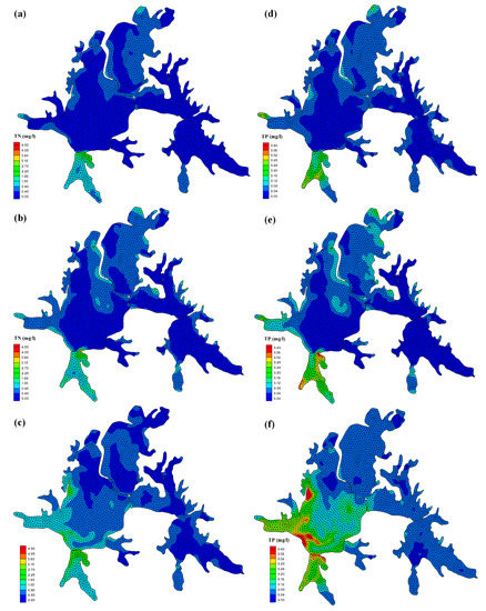
Figure 13.
(a–c): spatial distribution of TN under scenarios S1, S2, and S3; (d–f): spatial distribution of TP under scenarios S1, S2, and S3.
Water quality improvements are characterized by four indicators as shown in Table 6. Under scenarios S1, S2, and S3, TN concentrations are reduced by 35.8%, 43.2%, and 17.3%, respectively, and TP concentrations are reduced by 52.5%, 41.7% and 16.7%, respectively. Thus, it can be seen that scenario S1 is the best for reducing the TP concentration and that S2 is the best for reducing the TN concentration for the entire lake. According to the goal of the water diversion, the water quality in Lake Donghu must reach Class III. Based on the threshold values of TN and TP specified in Class III, the percentage of lake areas that failed to reach the goal was calculated and is presented in Table 6. Overall, scenarios S1 and S2 have similar effects towards improving water quality, and they outperform scenario S3 with respect to all indicators.
Table 6.
Water quality indicators under different water diversion scenarios.
Through a comprehensive consideration of hydrodynamic and water quality indicators, we can conclude the following: scenario S1 is the best for improving hydrodynamic indicators and for reducing TP concentrations, and scenario S2 is the best for reducing TN concentrations. Considering that TP is the major controlling factor for improving water quality for Lake Donghu, scenario S1 is thought to be the best solution to achieve the water diversion goal.
5. Conclusions
In this study, we illustrated the design and development of a visual modeling system, named the Lake Modeling System (LMS), streamlined for pre- and postprocessing of three-dimensional hydrodynamic and water quality modeling for lakes. The LMS provides a GIS-based environment to set up hydrodynamic and water quality models, as well as visualize and analyze model inputs/outputs. The application of the LMS in creating and interpreting the model input and output information improves the understanding of the hydrodynamic process and transport of pollutants in lakes, therefore promoting better decision-making in lake water resource management.
The case study in Lake Donghu demonstrated the applicability and effectiveness of the LMS for establishing a complex three-dimensional hydrodynamic and water quality model through a simple and easy-to-use graphic user interface. The Lake Donghu model established with LMS was used to simulate and compare three water diversion scenarios. The change of lake circulation pattern and improvement of water quality under different scenarios were also analyzed through postprocessing tools of LMS. The conclusions drawn from the case study illustrated that LMS could be used in real-world practices. However, in comparison with Delft3D and EFDC, the performance and abilities to simulate complicated water quality process of LMS is rather limited. To overcome this limitation, some advanced water quality modules will be incorporated into LMS. Although the current version of LMS was specially developed for FVCOM-LAKE, it can be easily extended to adapt to other hydrodynamic models. In future studies, we will extend LMS to make it support more models.
Author Contributions
Conceptualization: Y.T.; funding acquisition: M.H.; methodology: M.H.; software: Y.T. and M.H.; writing—original draft: M.H.; writing—review and editing: Y.T.
Funding
This research was funded by the National Natural Science Foundation of China (no. 51579108), the Shenzhen Science and Technology Innovation Commission (JCYJ20160530190547253), the National Key R and D Program of China (no. 2017YFC0405900), and the Fundamental Research Funds for the Central Universities under Grant (no. 2017KFYXJJ203). Additional support was provided by the Guangdong Provincial Key Laboratory of Soil and Groundwater Pollution Control (no. 2017B030301012) and the State Environmental Protection Key Laboratory of Integrated Surface Water-Groundwater Pollution Control.
Conflicts of Interest
The authors declare no conflict of interest.
References
- Burlakova, L.E.; Kovalenko, K.E.; Schmude, K.L.; Barbiero, R.P.; Karatayev, A.Y.; Lesht, B.M. Development of new indices of Great Lakes water quality based on profundal benthic communities. J. Gt. Lakes Res. 2018, 44, 618–628. [Google Scholar] [CrossRef]
- Huang, J.; Xu, Q.; Xi, B.; Wang, X.; Li, W.; Gao, G.; Huo, S.; Xia, X.; Jiang, T.; Ji, D.; et al. Impacts of hydrodynamic disturbance on sediment resuspension, phosphorus and phosphatase release, and cyanobacterial growth in Lake Tai. Environ. Earth Sci. 2015, 74, 3945–3954. [Google Scholar] [CrossRef]
- Nyamweya, C.; Sturludottir, E.; Tomasson, T.; Fulton, E.A.; Taabu-Munyaho, A.; Njiru, M.; Stefansson, G. Exploring Lake Victoria ecosystem functioning using the Atlantis modeling framework. Environ. Model. Softw. 2016, 86, 158–167. [Google Scholar] [CrossRef]
- Chen, C.S.; Liu, H.D.; Beardsley, R.C. An unstructured grid, finite-volume, three-dimensional, primitive equations ocean model: Application to coastal ocean and estuaries. J. Atmos. Ocean. Technol. 2003, 20, 159–186. [Google Scholar] [CrossRef]
- Bravo, H.R.; McLellan, S.L.; Klump, J.V.; Hamidi, S.A.; Talarczyk, D. Modeling the fecal coliform footprint in a Lake Michigan urban coastal area. Environ. Model. Softw. 2017, 95, 401–419. [Google Scholar] [CrossRef]
- Lesser, G.R.; Roelvink, J.A.; van Kester, J.; Stelling, G.S. Development and validation of a three-dimensional morphological model. Coast. Eng. 2004, 51, 883–915. [Google Scholar] [CrossRef]
- Luo, X.; Li, X. Using the EFDC model to evaluate the risks of eutrophication in an urban constructed pond from different water supply strategies. Ecol. Model. 2018, 372, 1–11. [Google Scholar] [CrossRef]
- Lu, C.; Li, H.; Dai, W.; Tao, J.; Xu, F.; Cybele, S.; Zhang, X.; Guo, H. 3-D Simulation of the Suspended Sediment Transport in the Jiao jiang Estuary: Based on Validating by Remote Sensing Retrieval. J. Coast. Res. 2018, 85, 116–120. [Google Scholar] [CrossRef]
- Beletsky, D.; Hawley, N.; Rao, Y.R. Modeling summer circulation and thermal structure of Lake Erie. J. Geophys. Res. Oceans 2013, 118, 6238–6252. [Google Scholar] [CrossRef]
- Bai, X.; Wang, J.; Schwab, D.J.; Yang, Y.; Luo, L.; Leshkevich, G.A.; Liu, S. Modeling 1993-2008 climatology of seasonal general circulation and thermal structure in the Great Lakes using FVCOM. Ocean Model. 2013, 65, 40–63. [Google Scholar] [CrossRef]
- Shore, J.A. Modelling the circulation and exchange of Kingston Basin and Lake Ontario with FVCOM. Ocean Model. 2009, 30, 106–114. [Google Scholar] [CrossRef]
- Huang, J.; Zhang, Y.; Huang, Q.; Gao, J. When and where to reduce nutrient for controlling harmful algal blooms in large eutrophic lake Chaohu, China? Ecol. Indic. 2018, 89, 808–817. [Google Scholar] [CrossRef]
- Gong, R.; Xu, L.; Wang, D.; Li, H.; Xu, J. Water Quality Modeling for a Typical Urban Lake Based on the EFDC Model. Environ. Model. Assess. 2016, 21, 643–655. [Google Scholar] [CrossRef]
- Liang, S.X.; Xie, J.; Sun, Z.C.; Lu, Y.P.; Liu, G.S.; Xiong, W. Development of a regional coastal management decision-aided system. Part A: Establishment of an automatic numerical simulation program. Ocean Coast. Manag. 2014, 96, 173–180. [Google Scholar] [CrossRef]
- Ng, S.M.Y.; Wai, O.W.H.; Li, Y.S.; Li, Z.L.; Jiang, Y.W. Integration of a GIS and a complex three-dimensional hydrodynamic, sediment and heavy metal transport numerical model. Adv. Eng. Softw. 2009, 40, 391–401. [Google Scholar] [CrossRef]
- Qin, R.F.; Lin, L.Z. Development of a GIS-based integrated framework for coastal seiches monitoring and forecasting: A North Jiangsu shoal case study. Comput. Geosci. 2017, 103, 70–79. [Google Scholar] [CrossRef]
- Tian, Y.; Zheng, Y.; Zheng, C.M. Development of a visualization tool for integrated surface water-groundwater modeling. Comput. Geosci. 2016, 86, 1–14. [Google Scholar] [CrossRef]
- Chen, C.S.; Huang, H.S.; Beardsley, R.C.; Liu, H.D.; Xu, Q.C.; Cowles, G. A finite volume numerical approach for coastal ocean circulation studies: Comparisons with finite difference models. J. Geophys. Res. Oceans 2007, 112, C03018. [Google Scholar] [CrossRef]
- Rego, J.L.; Li, C.Y. Storm surge propagation in Galveston Bay during Hurricane Ike. J. Mar. Syst. 2010, 82, 265–279. [Google Scholar] [CrossRef]
- Galperin, B.; Kantha, L.H.; Hassid, S.; Rosati, A. A Quasi-Equilibrium Turbulent Energy-Model for Geophysical Flows. J. Atmos. Sci. 1988, 45, 55–62. [Google Scholar] [CrossRef]
- Mellor, G.; Yamada, T. Development of a Turbulence Closure-Model for Geophysical Fluid Problems. Rev. Geophys. 1982, 20, 851–875. [Google Scholar] [CrossRef]
- Mellor, G.; Blumberg, A. Wave breaking and ocean surface layer thermal response. J. Phys. Oceanogr. 2004, 34, 693–698. [Google Scholar] [CrossRef]
- Ambrose, J.R.B.; Wool, T.A.; Connolly, J.P.; Schanz, R.W. A Hydrodynamic and Water Quality Model: Model Theory, User’s Manual and Programmer’s Guide; U.S. Environmental Protection Agency: Athens, GA, USA, 1988; pp. 280–297.
- Zheng, L.Y.; Chen, C.S.; Zhang, F.Y. Development of water quality model in the Satilla River Estuary, Georgia. Eco. Model. 2004, 178, 457–482. [Google Scholar] [CrossRef]
- DotSpatial. Available online: https://github.com/DotSpatial/DotSpatial (accessed on 6 January 2019).
- Shewchuk, J.R. Delaunay refinement algorithms for triangular mesh generation. Comput. Geom. 2002, 22, 21–74. [Google Scholar] [CrossRef]
- State Environment Protection Administration (SEPA). Environmental Quality Standard for Surface Water, China; GB 3838–2002; General Administration for Quality Supervision, Inspection and Quarantine of PR China: Beijing, China, 2002; pp. 1–9. Available online: http://kjs.mee.gov.cn/hjbhbz/bzwb/shjbh/shjzlbz/200206/t20020601_66497.shtml (accessed on 6 January 2019).
- Li, Y.P.; Acharya, K.; Yu, Z.B. Modeling impacts of Yangtze River water transfer on water ages in Lake Taihu, China. Ecol. Eng. 2011, 37, 325–334. [Google Scholar] [CrossRef]
- Chen, X.; Yang, X.; Dong, X.; Liu, Q. Nutrient dynamics linked to hydrological condition and anthropogenic nutrient loading in Chaohu Lake (southeast China). Hydrobiologia 2011, 661, 223–234. [Google Scholar] [CrossRef]
- Chen, Q.W.; Tan, K.; Zhu, C.B.; Li, R.N. Development and application of a two-dimensional water quality model for the Daqinghe River Mouth of the Dianchi Lake. J. Environ. Sci. 2009, 21, 313–318. [Google Scholar] [CrossRef]
- Dortch, Q. The interaction between ammonium and nitrate uptake in phytoplankton. Mar. Ecol. Prog. Ser. 1990, 61, 183–201. [Google Scholar] [CrossRef]
- Geider, R.J. Respiration: Taxation without representation. In Primary Productivity and Biogeochemical Cycles in the Sea; Falkowski, P.G., Woodhead, A.D., Eds.; Plenum Press: New York, NY, USA, 1992; pp. 333–360. [Google Scholar]
- Stenstrom, M.K.; Poduska, R.A. The Effect of Dissolved-Oxygen Concentration on Nitrification. Water Res. 1980, 14, 643–649. [Google Scholar] [CrossRef]
© 2019 by the authors. Licensee MDPI, Basel, Switzerland. This article is an open access article distributed under the terms and conditions of the Creative Commons Attribution (CC BY) license (http://creativecommons.org/licenses/by/4.0/).