Joint Alternate Small Convolution and Feature Reuse for Hyperspectral Image Classification

Abstract

A hyperspectral image (HSI) contains fine and rich spectral information and spatial information of ground objects, which has great potential in applications. It is also widely used in precision agriculture, marine monitoring, military reconnaissance and many other fields. In recent years, a convolutional neural network (CNN) has been successfully used in HSI classification and has provided it with outstanding capacity for improving classification effects. To get rid of the bondage of strong correlation among bands for HSI classification, an effective CNN architecture is proposed for HSI classification in this work. The proposed CNN architecture has several distinct advantages. First, each 1D spectral vector that corresponds to a pixel in an HSI is transformed into a 2D spectral feature matrix, thereby emphasizing the difference among samples. In addition, this architecture can not only weaken the influence of strong correlation among bands on classification, but can also fully utilize the spectral information of hyperspectral data. Furthermore, a 1 × 1 convolutional layer is adopted to better deal with HSI information. All the convolutional layers in the proposed CNN architecture are composed of small convolutional kernels. Moreover, cascaded composite layers of the architecture consist of 1 × 1 and 3 × 3 convolutional layers. The inputs and outputs of each composite layer are stitched as the inputs of the next composite layer, thereby accomplishing feature reuse. This special module with joint alternate small convolution and feature reuse can extract high-level features from hyperspectral data meticulously and comprehensively solve the overfitting problem to an extent, in order to obtain a considerable classification effect. Finally, global average pooling is used to replace the traditional fully connected layer to reduce the model parameters and extract high-dimensional features from the hyperspectral data at the end of the architecture. Experimental results on three benchmark HSI datasets show the high classification accuracy and effectiveness of the proposed method.

1. Introduction

Hyperspectral remote-sensing technology has been an important part of comprehensive Earth observation research since the 1980s. It is also a key point in the competition for international Earth observation technology. In addition, the applications of this technology have been gradually extended to many fields, such as environmental monitoring, land use, resource investigation, and atmospheric research. Hyperspectral image (HSI) data have the characteristics of combining images and spectra, that is, each pixel on an HSI corresponds to a spectral curve. The class of ground truth can be identified on the basis of its spectral reflectance because of the aforementioned characteristics. Each pixel in an HSI corresponds to hundreds or even thousands of bands. Moreover, the spectral resolution of HSI reaches nanoscale and contains abundant and detailed ground truth information. However, traditional multispectral data contain only a few spectral bands and have low spectral resolution. Therefore, the use of hyperspectral data is more advantageous than that of multispectral data in identifying and classifying ground truth. With hyperspectral data, a substantial variety of fine ground truth can be identified, and various samples and band combinations can be selected flexibly to obtain different features and fulfill varying task demands during ground truth recognition and classification. Furthermore, with the development of big data technology, HSI will have a bright future in big data research in remote sensing because of its considerable potential application value.

HSIs bring substantial opportunities to ground truth recognition and classification because of their rich information but remain a challenge to traditional remote-sensing image classification methods due to the large number of bands and insufficient training samples of HSI data. On the one hand, with the increase of band number, the classification accuracy obtained by directly using the information of all the bands is likely to decrease, that is, the so-called Hughes phenomenon [1]. On the other hand, classification speed also restricts the application of HSIs as the number of bands increases. Many research institutions and related scholars have explored HSI classification in theory and application and proposed many mature and classic HSI classification methods to fully utilize the advantages of hyperspectral remote-sensing technology. From the perspective of HSI description space, HSI classification methods can be divided into two categories [2]: the methods based on spectral space and those based on feature space. The former utilizes the spectral curve that can reflect the spectral feature of ground truth to identify the ground truth. This kind of method include minimum distance spectrum matching, and spectral angle matching. The latter utilizes the statistical characteristics of ground truth in the feature space to build classification models, and representative methods, including the decision tree [3], artificial neural network (ANN) method [4], and support vector machine (SVM) classification [5]. The ground truth that corresponds to the same pixel is not unique, and many mixed pixels exist due to “same objects with different spectrum, different objects with same spectrum” phenomenon and the low spatial resolution of HSI. Moreover, the classification accuracy of the methods based on spectral space is seriously affected. By contrast, classification methods based on feature space are not constrained by these factors and hence favored by scholars. For instance, Sun et al. [5] proposed a band-weighted SVM (BWSVM) method to classify HSIs. Li et al. [6] adopted a radial basis function to implement a kernel extreme learning machine (KELM), which provided better classification performance on the HSI than kernel SVM. Wei et al. [7] functionalized hyperspectral pixels, adopted functional principal component analysis (KPCA) to reduce the dimensionality of functional data, and classified the reduced-dimensionality data by KELM. Although scholars have attained many excellent research achievements in HSI classification, the characteristics of hyperspectral data, such as high dimension, large computation, and strong correlation among bands, still restrict traditional methods from improving classification accuracy. Furthermore, due to the shallow structure, the above methods are equipped with limit ability of feature extraction. Therefore, their classification performance for HSIs makes it easy to encounter bottlenecks. The convolutional neural network (CNN), with its deep structure and end-to-end learning mode, is provided with strong learning capability for features. In such a learning mode, the low-level features are abstracted layer by layer to the high-level features required by relevant tasks. Particularly, CNNs have demonstrated remarkable performance in image classification and target detection [8,9,10], which undoubtedly represent the gospel for improving the classification performance of HSI effectively.

A CNN is a special feedforward ANN. About 20 years ago, LeCun et al. [11] trained a CNN using the back-propagation algorithm and the gradient learning technique and then demonstrated its effectiveness through a handwritten digit recognition task. However, the development of CNN subsequently declined due to the constraints of computing power and difficulties in theoretical analysis for neural networks. In 2012, Hinton et al. [12] succeed at image classification challenge of ImageNet with Alex-Net, whose accuracy was approximately 12% higher than that of the immediate runner-up. Since then, CNNs such as NIN (Network in Network) [13], GoogLeNet [14], DeepID2+ [15], and ResNet [16] have made great historical breakthroughs and drawn a resurgence of attention to various visual recognition tasks. CNNs are being increasingly applied to HSI classification. For example, Chen et al. [17] exploited a CNN to extract the deep features of hyperspectral data and committed to solve the problems of high-dimensional and limited samples in hyperspectral data. Yue et al. [18] proposed a new classification framework composed of exponential momentum deep CNN and SVM. This framework can construct high-level spectral–spatial features hierarchically in an automated manner. Hu et al. [19] proposed a CNN model to classify HSIs directly in the spectral domain, whose CNN architecture only contains one convolutional layer and one fully connected layer, which may be hard to effectively extract robust spectral features from when the number of training samples per class is small. The 3D-CNN was also applied to hyperspectral classification [20,21,22], which can extract spectral and spatial features simultaneously and was provided with excellent classification performance. Makantasis et al. [23] encoded spatial and spectral information of hyperspectral images with CNN, and adopted randomized PCA along the spectral dimension to reduce the dimensionality of input raw data, which is a good idea. The use of CNNs effectively improves HSI classification. However, the strong correlation among bands in hyperspectral data, which is also an important factor that restricts the improvement of HSI classification accuracy, has rarely been studied. Furthermore, the CNN application technology in HSI classification is not mature enough, and such shortcomings as weak generalization capability and easy overfitting remain.

A new deep CNN architecture that realizes the classification task by learning the hyperspectral data features layer by layer is proposed in this research to solve the aforementioned problem. The major contributions of this work can be summarized as follows.

• Unlike existing HSI classification methods, this work transforms the 1D spectral vectors of hyperspectral data into 2D spectral feature matrices. The spectral features are mapped from 1D to 2D space. And the variations among different samples, especially those among samples from various classes, are highlighted. This work enables the CNN to fully use the spectral information from each band and extract the spectral features of the hyperspectral data accurately. Meanwhile, the interference of highly correlated bands for HSI classification can be weakened.
• The entire network architecture adopts small convolution kernels with size of 3 × 3 or 1 × 1 to form convolutional layers. The conversion of the 1D spectral vector to a 2D spectral feature matrix can weaken the interference of highly correlated bands for HSI classification, but cannot eliminate the correlation among bands. Adopting convolutional kernels with different sizes allows the acquisition of local receptive fields with varying sizes. After multilayer abstraction, the correlation among different spectral bands is gradually weakened. The entire network can learn the features of HSIs meticulously and robustly. Furthermore, cascaded 1 × 1 convolutional layers can increase the non-linearity of the network and make the spectral features of the hyperspectral data increasingly abstract. Simultaneously, the correlation among bands in the hyperspectral data can be weakened and the features of hyperspectral data can be learned effectively.
• 1 × 1 and 3 × 3 convolutional layers are cascaded to form a special composite layer. The 1 × 1 convolutional layer can integrate high-level spectral features output by the front layer from a global perspective and increasing the compactness of the proposed CNN architecture. The 3 × 3 convolutional layer can deeply learn the features integrated by the 1 × 1 convolutional layer in detail from multiple local perspectives. Multiple composite layers are cascaded so that 1 × 1 and 3 × 3 convolutional layers are stacked in the network alternately. In a cross-layer connection, the input and output of each composite layer are spliced into new features in the feature dimension and passed to the next composite layer, thus accomplishing feature reuse. This combination of alternating small convolutions and feature reuse is called the ASC–FR module. When extracting the features of hyperspectral data, the ASC–FR module can constantly switch the perspective of extraction between the global and local perspectives. Therefore, this module ensures that the spectral features can be fully utilized after multilayer abstraction, the deep features of hyperspectral data are extracted comprehensively and meticulously, and the adverse effects of strong correlation among bands on classification are weakened. To a certain extent, the overfitting and gradient disappearance in the proposed CNN architecture are solved. Thus, this module can improve the accuracy of HSI classification effectively.

The remainder of this paper is organized as follows. Section 2 briefly introduces the advantages of the small convolution kernel and describes some of the relevant work about CNN-based HSI classification. Section 3 describes the overall design of the proposed method. Section 4 evaluates the classification performance of this work through comparative experiments and analyses. Section 5 concludes the paper.

2. Related Work

2.1. Small Convolution

Generally, a CNN contains the input layer, the convolutional layer, the pooling layer, the fully connected layer and the output layer. Each convolutional layer comprises several convolutional kernels, which can extract the local features from input feature maps. Small convolutional kernels (3 × 3 or 5 × 5) have more advantages than large ones. Through multilayer stacking, small convolutional kernels can provide the receptive field with the same size as that provided by large convolutional kernels. Moreover, the use of small convolutional kernels can bring two advantages. First, stacking multiple layers that consist of small convolutional kernels can increase the network depth, thereby enhancing the capacity and complexity of the network. Second, the model parameters can be reduced effectively by using small convolution in the model. In VGG-Net [24], which was proposed by the Oxford Visual Geometry Group of the University of Oxford, all convolutional layers adopt 3 × 3 convolutional kernels, thus possibly reducing network parameters effectively and enhancing the fitting capability of the network. As for a smaller convolutional kernel, the 1 × 1 sized convolutional kernel, its capacity was first discovered in the NIN [13] in 2014. This network has a multilayer perceptron convolutional (mlpconv) layer, which is a cascaded cross-channel parametric pooling (CCCP) on a normal convolutional layer. This CCCP structure allows the network to learn complex and useful cross-channel integration features. The CCCP layer is equivalent to a convolutional layer with 1 × 1 convolutional kernels. After the appearance of NIN, GoogLeNet, ResNet and their families also widely adopted small convolutional kernels and demonstrated that such kernels can greatly improve the capability of networks for learning features.

2.2. Convolutional Neural Network (CNN)-Based Classification for Hyperspectral Image (HSI)

CNN has demonstrated remarkable performance in HSI classification, denoising [25], segmentation [26] and so on. After summarizing the research works of CNN in HSI classification, according to the way of implementation, the HSI classification method based on CNN can be divided into 1D-CNN-based, 2D-CNN-based and 3D-CNN-based methods, and the method combining CNN with other approaches. Among them, the method based on 1D-CNN [17,19] usually assumes that each pixel in an HSI only corresponds to one class, and directly uses 1D spectral information for hyperspectral classification. Although this kind of methods are easy to implement, they are seriously affected by mixed pixels and strong correlation among bands, which causes that the model cannot effectively learn the spectral features of each pixel, and is provided with poor adaptability. The method based on 2D-CNN [27,28] usually adopts some approaches (such as principal component analysis, autoencoder) to extract the main components of spectral information in advance, and then extract neighborhood pixel blocks from the image as samples. The 3D-CNN based method utilizes pixel cube to implement hyperspectral classification [20,21,22]. Both the two kinds of methods introduce spatial information, which enables the model to learn more useful features and significantly improve the classification effect. However, these two kinds of methods require a large number of labeled pixels to generate sufficient samples for training the CNN model, coupled with the limited number of labeled pixels in HSIs, which aggravates the shortage of training samples and makes the model easy to over-fit. The two kinds of methods usually assume that the pixels in the same spatial neighborhood have similar spectral characteristics with the central pixels, and those pixels belong to the same class as the central pixel. It is ignored that the pixels in the same neighborhood may represent a different class of ground truth, that is, it is impossible to ensure that only one class of objects is included in the same neighborhood. Therefore, if the spatial size of the neighborhood pixel blocks is large, the two kinds of methods will be disturbed by heterogeneous noise (the pixels in a neighborhood pixel block belong to different class from the central pixel). The last kind of method [29,30] usually combines other approaches with CNN, which uses other approaches to make up for some shortcomings of CNN in HSI classification, so as to improve the classification performance of the CNN model. This kind of method requires fully excavating the characteristics of the CNN, and requires deep theoretical study. The implementation process is relatively tedious, but the performance is often excellent.

3. HSI Classification Method Based on Alternating Small Convolutions and Feature Reuse (ASC–FR)

3.1. Data Pre-processing

Hyperspectral data contain large number of bands and rich spectral values. Considering these characteristics, the 1D spectral vector is converted into the 2D feature matrix. Then, each pixel in the original HSI corresponds to a spectral feature map, and the difference among samples becomes increasingly remarkable. Inputting the spectral feature map into CNNs not only makes the network learn the spectral features of hyperspectral data effectively, but also reduces the influence of highly correlated bands on HSI classification. Moreover, the bondage of the high-dimension characteristic of hyperspectral data in the classification can be removed. Therefore, this data pre-processing technique can improve the classification accuracy effectively. The procedure of data pre-processing is displayed in Figure 1. It is noted that a few bands should be removed before transforming the spectral vector into the feature map. Removing a few bands can eliminate redundant information, weaken the correlation among bands of the data, and enhance the inter class separability. It also brings advantages to improvement of HSI classification accuracy. However, if too many bands are removed, some useful information will be lost, and the classification performance of the model will be degraded. Therefore, it is necessary to reasonably control the number of removed bands to make the advantages outweigh the disadvantages. Moreover, in order to convert the 1D spectral vector into the spectral feature map, the number of reserved bands should be a square number.

3.2. Proposed CNN Architecture

In the process of designing the network structure in this work, improving the HSI classification accuracy is considered as a goal. Meanwhile, deepening the abstraction of hyperspectral data features and avoiding the gradient disappearance and overfitting of the network as far as possible are considered as the main principles. The proposed CNN architecture is shown in Figure 2. At the input end, three 3 × 3 convolutional layers are stacked, followed by two cascaded 1 × 1 convolution layers, that is, the mlpconv layer. This layer can enhance the complexity of this network and make the features of hyperspectral data increasingly abstract. Then, the output features are integrated by overlapping max pooling and forwarding to the two cascaded composite layers. The obtained features are then transmitted to a 1 × 1 convolution layer and an average pooling layer. Finally, global average pooling (GAP) is adopted to deal with the whole feature map, and classification results are outputted by Softmax layer. The outputs of each convolutional layer are treated with batch normalization (BN) and rectified linear unit (ReLU) in turn, that is, Conv → BN → ReLU.

Width expansion rate. In this work, the width (channel number) of each convolution layer is set as a multiple of g. The width of the network increases with g, which is thus called the width expansion rate. Different width expansion rates indicate that the number of new feature information received by each layer varies. Therefore, the width of the network can be adjusted and the efficiency of the network parameters can be improved by an adjustment of the width expansion rate. In the experiment, the output dimension of nearly all the convolution layers, except the composite layers, are set as 2g to adjust the width and depth of network conveniently.

ASC–FR module. The composite layer consists of 1 × 1 and 3 × 3 convolution layers, where the output dimensions of both 1 × 1 and 3 × 3 convolution layers are set as 4g. In this manner, the output dimension of each composite layer is maintained and the expansion of the network is facilitated. Through a stitching operation, the input and output features of each composite layer are combined as new features that form the input of the next composite layer. This operation leads to feature reuse, which is helpful in preventing overfitting. The aforementioned information is the detail of the ASC–FR module. When the feature dimension is high after splicing, the composite layer can reduce the dimension of features, thereby increasing the compactness of the network structure and reducing the computation.

4. Experiments and Analysis

The proposed CNN architecture is implemented via TensorFlow1.4.2. The experiments are conducted on a desktop PC with Windows 7 64-bit OS, Inter(R) Core(TM) i5-4460 CPU, 8 GB RAM and NVIDIA GeForce GTX 1070 8G GPU. Three benchmark datasets are used to evaluate the classification performance of the proposed method. This section introduces the datasets, provides details about the experimental design, and conducts analyses according to the experimental results.

4.1. Datasets and Data Pre-Processing

4.1.1. Indian Pines Dataset

The Indian Pines image was captured by the AVIRIS sensor with a spatial resolution of 20 m over the Indian Pines test site in north-western Indiana. This image contains 145 × 145 pixels and 224 spectral reflectance bands, whose wavelength ranges from 0.4 μm to 2.5 μm. After discarding four zero bands, 220 bands are reserved. There are 16 ground-truth classes and 10,249 labeled pixels. Figure 3 displays the details of the Indian Pines image.

Table 1. Indian Pines image: the number of samples per class.

Class	Name	Number	Train	Test
C1	Alfalfa	46	10	36
C2	Corn-notill	1428	345	1083
C3	Corn-mintill	830	219	611
C4	Corn	237	64	173
C5	Grass-pasture	483	133	350
C6	Grass-trees	730	188	542
C7	Grass-pasture-mowed	28	7	21
C8	Hay-windrowed	478	115	363
C9	Oats	20	8	12
C10	Soybean-notill	972	243	729
C11	Soybean-mintill	2455	626	1829
C12	Soybean-clean	593	136	457
C13	Wheat	205	46	159
C14	Woods	1265	311	954
C15	Buildings-Grass-Trees-Drives	386	85	301
C16	Stone-Steel-Towers	93	26	67
Total		10,249	2562	7687

illustrates the number of samples per class in the Indian Pines dataset.

For the Indian Pines dataset, 20 bands that cover the region of water absorption and four bands with low signal-to-noise ratio (SNR), including [104–108,150–165,218–220], are removed. The 196 preserved bands are used for classification. Figure 4 displays the mean spectral signatures of the 16 ground-truth classes. The 1D spectral vector that corresponds to each sample is converted into a spectral feature map that contains 14 × 14 pixels. Then, the data are processed by zero mean treatment. Figure 5 shows the spectral feature maps of the 16 ground truth classes after quantizing spectral values at 20 levels. Figure 4 shows that the differences between different curves are noticeable in most bands, while being remarkably small in the other bands. A few spectral curves nearly coincide even in all the bands, and it is hard to distinguish them. In the process of classification, this situation will easily lead to the misclassification of some classes, which is not conducive to the improvement of overall classification accuracy. Therefore, training the network using 1D spectral vectors directly is not conducive to the extraction of features from the original data, thereby leading to an overfitting problem and poor overall classification performance of the proposed method. After converting the samples into 2D forms, spectral feature maps from different classes are easy to distinguish, as displayed in Figure 5. This illustrates that the data processing method is conducive to the network learning of the hyperspectral data features, thus improving the classification performance of the network.

4.1.2. Salinas Dataset

The Salinas image was collected by the AVIRIS (Airborne Visible Infrared Imaging Spectrometer) sensor with a spatial resolution of 3.7 m per pixel over Salinas Valley, California. This image contains 512 × 217 pixels, 224 spectral bands, and 16 ground truth classes. The details of the Salinas image are shown in Figure 6.

Table 2. Salinas image: the number of samples per class.

Class	Name	Number	Train	Test
C1	green_weeds_1	2009	524	1485
C2	green_weeds_2	3726	933	2793
C3	Fallow	1976	514	1462
C4	Fallow rough plow	1394	343	1051
C5	Fallow smooth	2678	671	2007
C6	Stubble	3959	977	2982
C7	Celery	3579	931	2648
C8	Grapes untrained	11,271	2826	8445
C9	Soil vinyard	6203	1536	4667
C10	Corn senesced	3278	813	2465
C11	Lettuce_romaine_4wk	1068	263	805
C12	Lettuce_romaine_5wk	1927	493	1434
C13	Lettuce_romaine_6wk	916	211	705
C14	Lettuce_romaine_7wk	1070	238	832
C15	Vinyard_untrained	7268	1806	5462
C16	Vinyard_vertical	1807	453	1354
Total		54,129	13,532	40,597

lists the number of samples per class.

For the Salinas dataset, 20 bands that cover the region of water absorption and 8 bands with low SNR, including [107–113,153–168,220–224], are removed. The 196 remaining bands are used for classification. The spectral vectors of the preserved data are transformed into feature maps with 14 × 14 pixels. The data are processed by zero mean treatment. Accordingly, the mean spectral signatures of 16 classes in the Salinas dataset are shown in Figure 7, and the spectral feature maps after quantizing spectral values at 20 levels are shown in Figure 8. Figure 7 and Figure 8 demonstrate that transforming the samples from 1D to 2D emphasizes the difference among the samples from various ground-truth classes for the Salinas dataset.

4.1.3. Pavia University Dataset

This HSI was captured by the ROSIS (Reflective Off-axis System Imaging Spectrometer) sensor with spatial resolution of 1.3 m over the Pavia University in northern Italy. It contains 103 spectral bands, 610 × 340 pixels and 9 ground-truth classes. Its details are shown in Figure 9.

Table 3. Pavia University image: the number of samples per class.

Class	Name	Number	Train	Test
C1	Asphalt	6631	1668	4963
C2	Meadows	18,649	4583	14,066
C3	Gravel	2099	512	1587
C4	Trees	3064	831	2233
C5	Painted metal sheets	1345	331	1014
C6	Bare Soil	5029	1270	3759
C7	Bitumen	1330	334	996
C8	Self-Blocking Bricks	3682	936	2746
C9	Shadows	947	229	718
Total		42,776	10,694	32,082

lists the number of samples per class in this image.

For the Pavia University image, only three bands were removed and 100 bands were retained to convert spectral vectors into feature maps because there exist obvious differences among different mean spectral curves (Figure 10). The corresponding spectral feature maps are shown in Figure 11 below.

4.2. Experimental Design

In this section, several comparative experiments are designed to evaluate the classification performance of the proposed method in HSI. The details of the experiments are as follows.

(1)

Comparison of classification performances of proposed method under different parameter settings. Two comparisons are needed because different width expansion rates (g) and network depths lead to varying classification performances of the proposed method. ① The number of composite layers is denoted as nc_layer and set as 2, and the classification performances of the proposed method when the value of g is 8/20/32 are compared. ② g is set as 20, and the classification performances of the proposed method when the value of nc_layer is 2/4/8 are compared.

(2)

Comparison with other methods. The classification performance of proposed method is compared with that of the deep learning method and non-deep learning method on the HSI.

In the training process, the training samples are divided into batches, and the number of samples per batch in our experiment is 64. For each epoch, the whole training set is learned by the proposed CNN. The total of epochs is 200 in each experiment. The Adam optimizer is applied to train the proposed CNN, and MSRA initialization method [31] is used for weight initialization. The parameter of the Adam optimizer, epsilon, is set as 1 ×10⁻⁸. The initial learning rate for the Indian Pines dataset is 1 ×10⁻², which is reduced 10/100/200 times when epoch = 20/60/100, respectively. For the Salinas dataset and the Pavia University dataset, the initial learning rate is 1 ×10⁻³, which is reduced 10/100/200 times when epoch = 40/100/150, respectively. If there is no special illustration, then all the parameters are set according to the aforementioned settings. These parameters may not be optimal, but at least effective for the proposed CNN.

Division of training set and test set. Generally, insufficient training samples will lead to serious overfitting of deep CNN models. However, the deep CNN model is equipped with strong feature extraction capacity due to its deep structure. Moreover, BN and MSRA initialization method are adopted for training the proposed CNN effectively, which improve the generalization performance of proposed CNN. Therefore, proposed method can extract deep features from small training samples set effectively. The limited available labeled pixels of HSI leads to insufficient training samples, which usually make it a challenge to improve the classification accuracy of the HSI. Considering this, to evaluate the effectiveness of proposed method under limited training samples, we randomly select 25% of samples in each HSI dataset for the training set, and the rest for the test set.

4.3. Experimental Results and Analyses

In this work, overall accuracy (OA), average accuracy (AA), and kappa coefficient (Kappa) are adopted to evaluate the classification performance of the proposed method in HSI data. Among them, OA refers to the ratio of the number of pixels correctly classified to the total number of all labeled pixels. AA is the average of classification accuracy of all classes. The Kappa coefficient is used to assess the agreement of classification for all the classes. The greater the kappa value, the better the overall classification effect. All the following data are the average of 10 experimental results under the same conditions to ensure the objectivity of the experimental results.

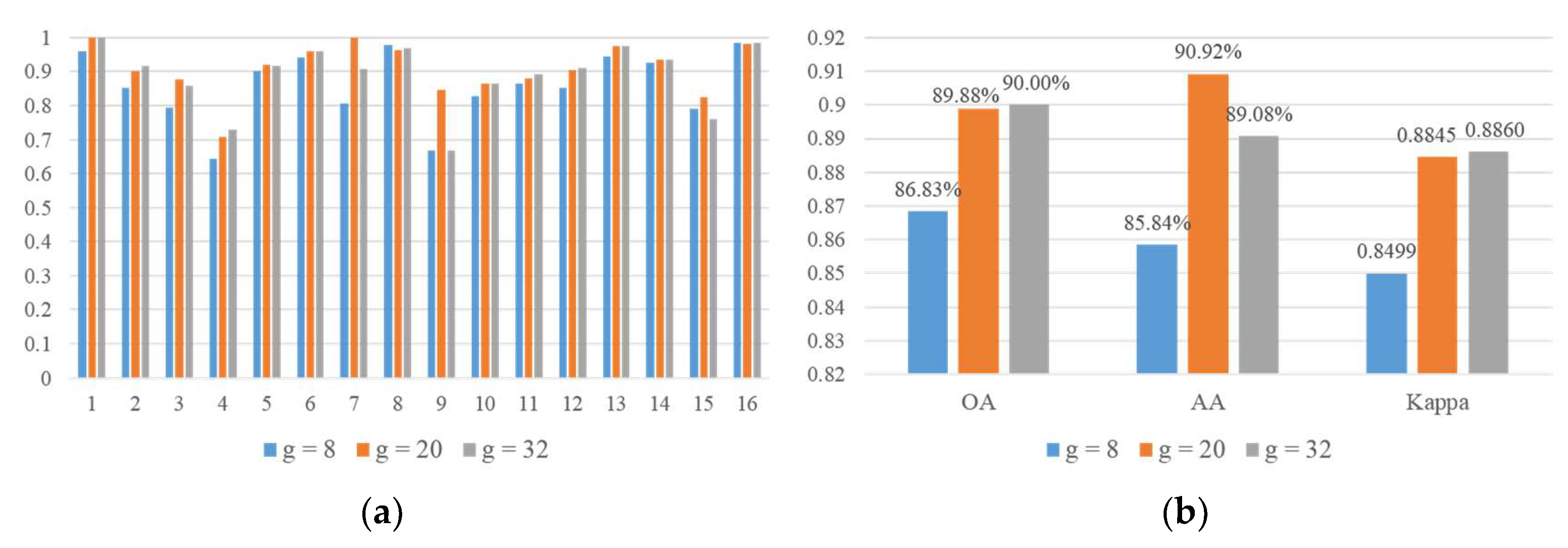
(1) Experimental Results in the Indian Pines Dataset

Classification performance of the proposed method under different width expansion rates: Figure 12 displays the bar of the classification results when nc_layer = 2 and g = 8/20/32. According to Figure 12, when the network depth is the same, the width of the network is increased gradually and the classification performance of the proposed method is improved gradually with the increase of width expansion rate (g). However, the trend of this improvement gradually saturates. OA/AA/Kappa are increased by 3.05%/5.08%/0.0346, respectively, when g is increased from 8 to 20. When g is increased from 20 to 32, OA and Kappa are almost invariable and AA is slightly reduced. Within a certain range, the increase of network width can lead to improving the feature extraction of hyperspectral data, thus enhancing classification accuracy. However, this improvement has an upper limit. Widening the network width will certainly increase the computation of the network, thereby increasing the time consumed by classification. Therefore, the width of the network should be controlled when designing the HSI classification method.

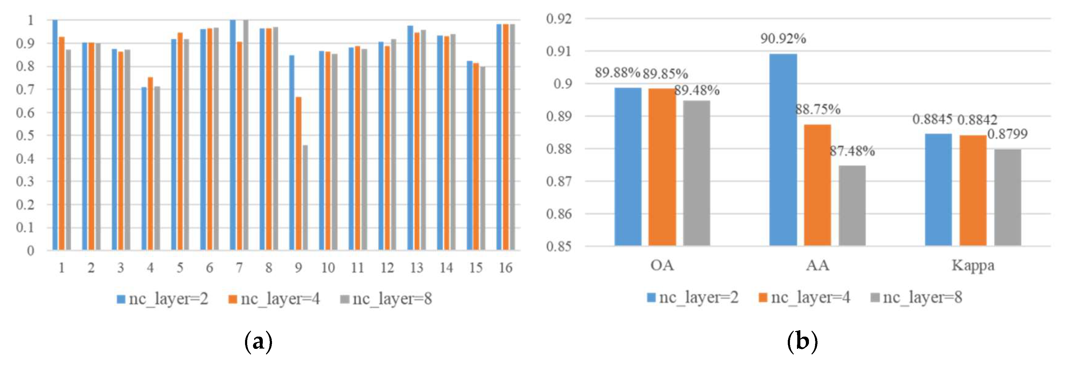
Classification performance of the proposed method under different number of composite layers. Figure 13 displays the bar of classification results when nc_layer = 2 and g = 8/20/32. Increasing the number of composite layers cannot increase the classification accuracy of the proposed method when the width expansion rate remains the same. An increase in network depth will greatly increase the computation of the network and prolong the time for network training. Considering the large computation of hyperspectral data, the network depth should be controlled on the premise of ensuring high classification accuracy.

In summary, in terms of classification accuracy and speed, setting g = 20 and nc_layer = 2 is suitable.

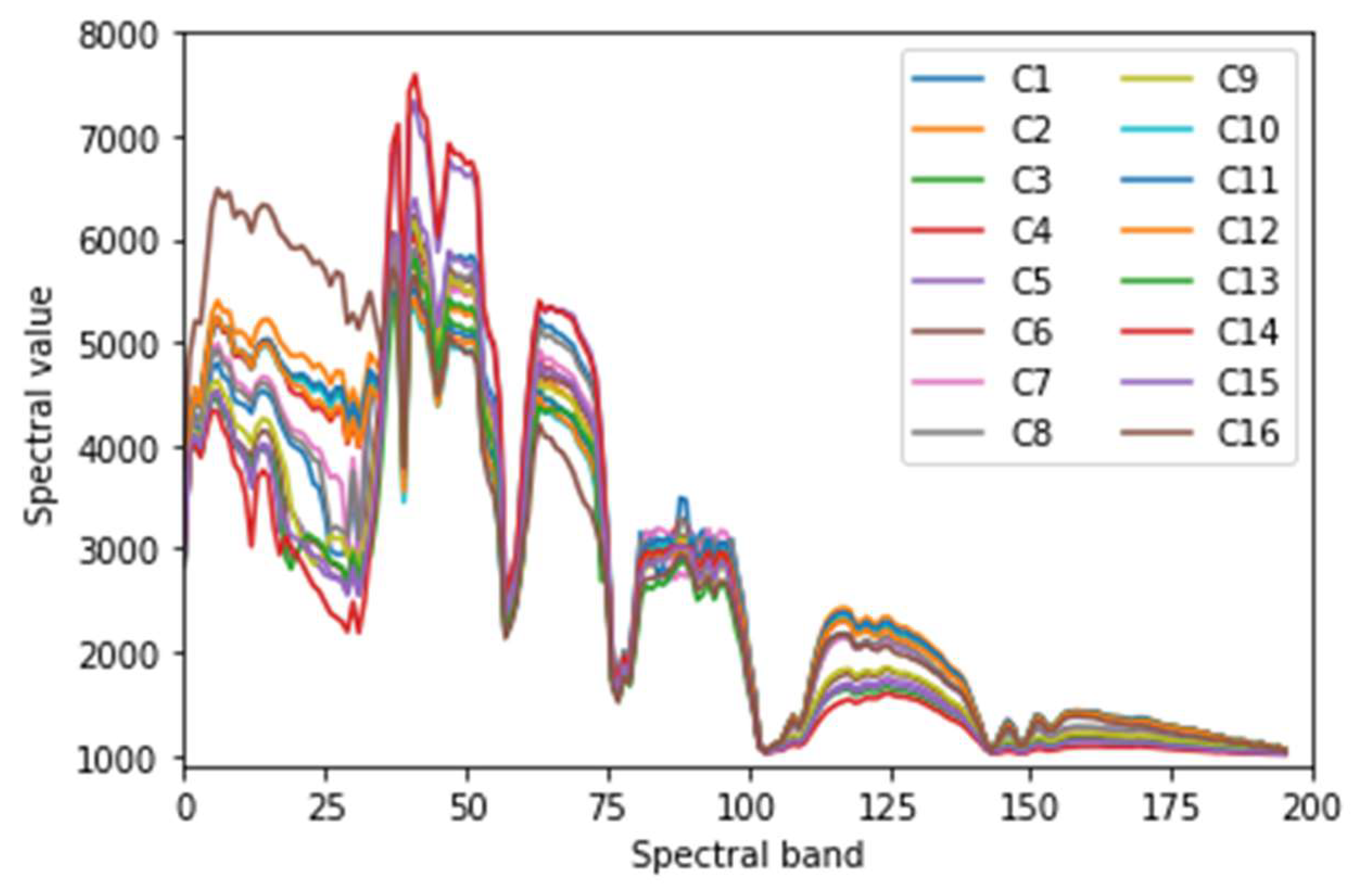
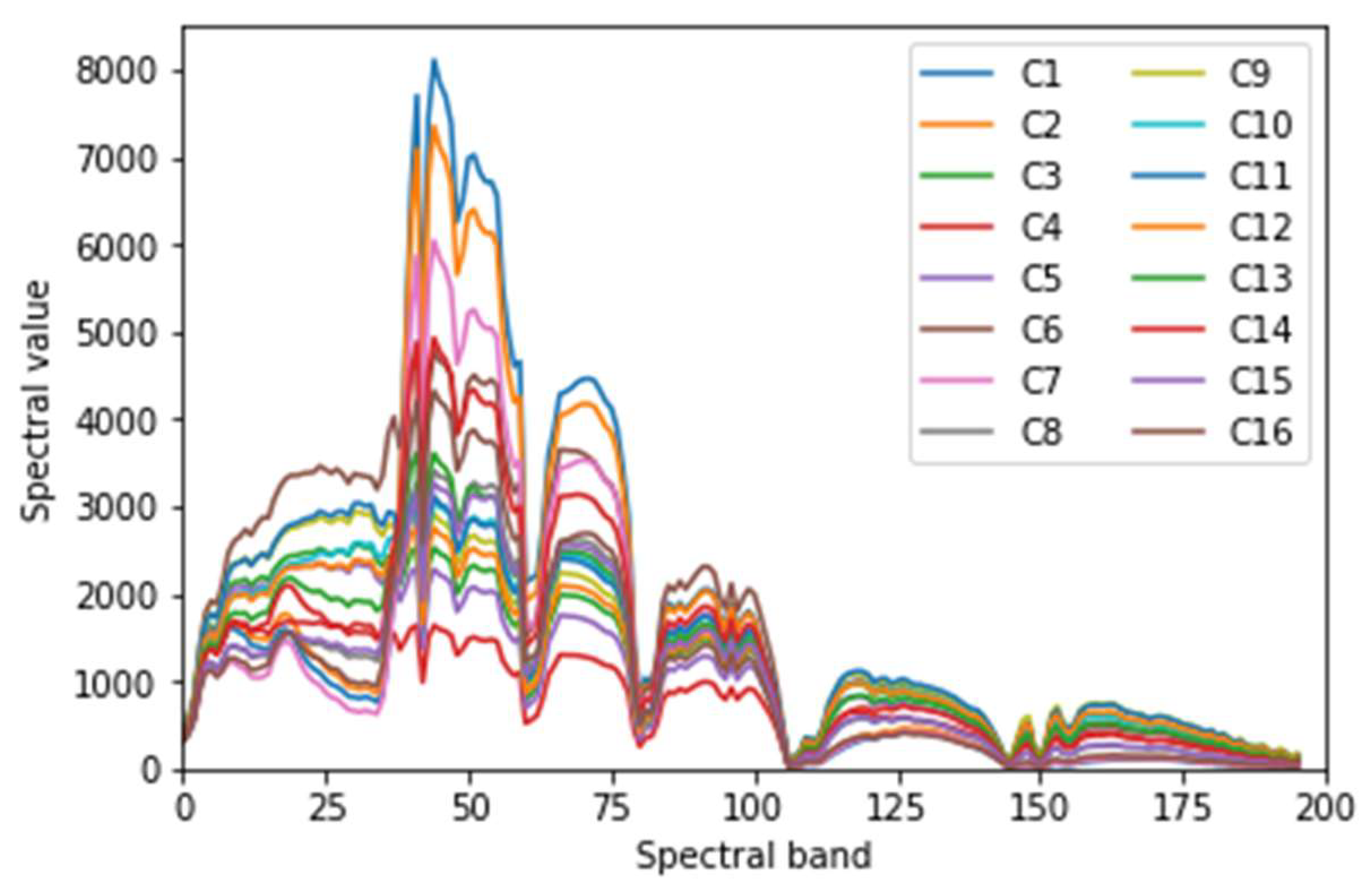
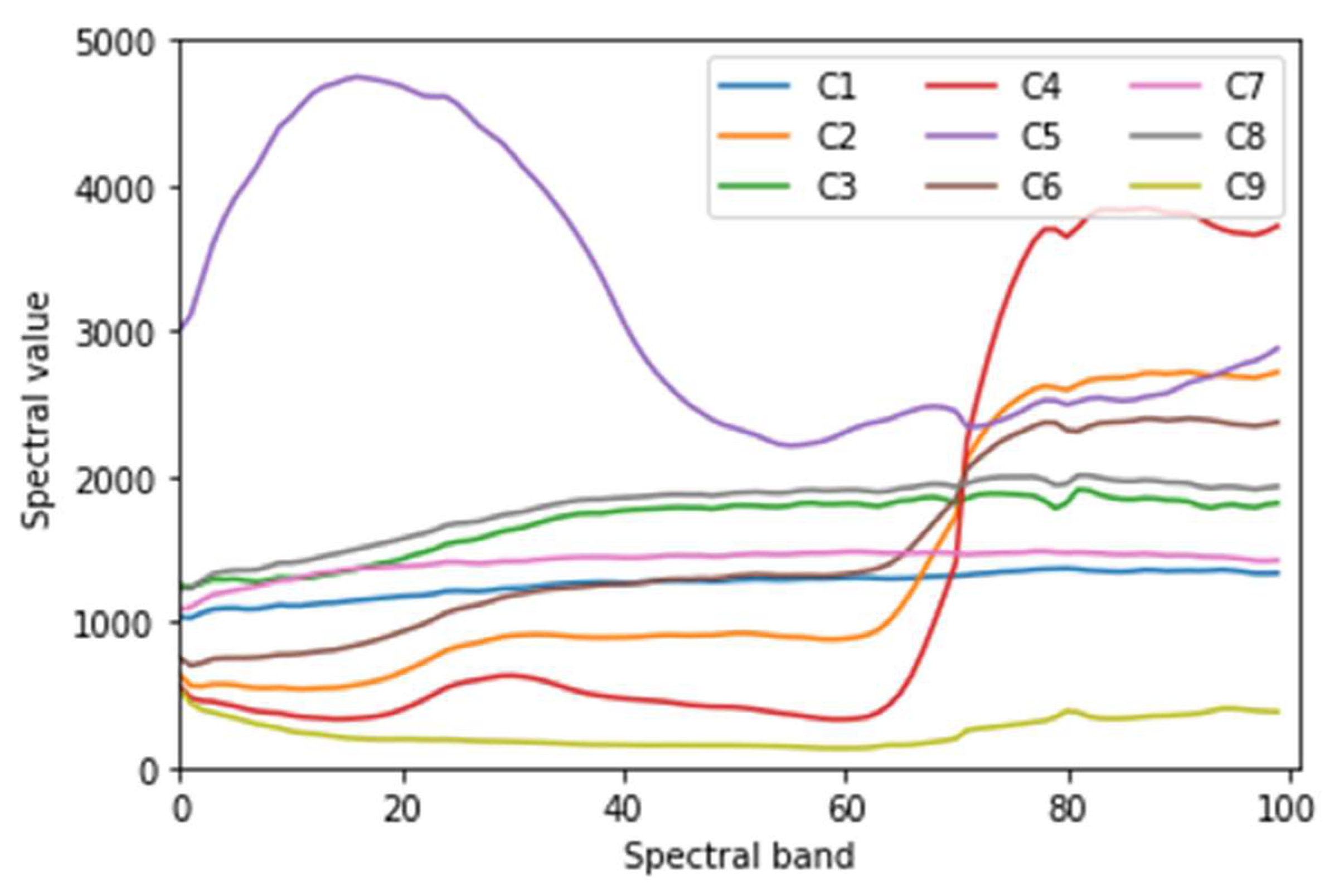
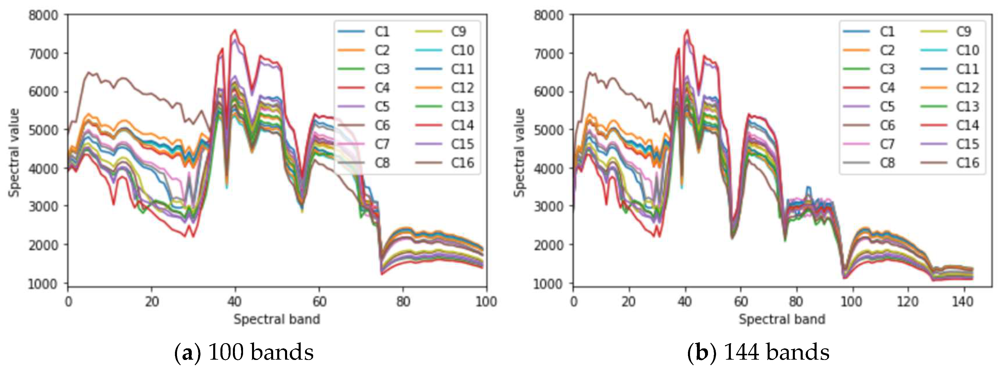
Impact of band number. As can be seen from Figure 4, when the number of reserved bands is 196, many spectral curves still have serious aliasing at some bands, which is unfavorable for classification. In order to obtain the optimal number of reserved bands, the classification results of 100, 144 and 196 bands under nc_layer = 2, g = 20 are compared (

Table 4. Classification results of different number of reserved bands in the Indian Pines dataset.

Band Number	OA	AA	Kappa
100	86.94%	85.73%	0.8510
144	89.76%	88.37%	0.8838
196	89.88%	90.92%	0.8845

). According to Figure 4 and Figure 14, after removing more bands, the aliasing of spectral curves is much less, which enhances the inter class separability of Indian Pines data effectively. Unfortunately, and simultaneously, it also leads to the loss of much useful information. The enhancement of inter class separability bring benefits to the improvement of classification accuracy, while the loss of useful information cause damage to the improvement of classification accuracy. For the reason that the disadvantage outweighs the advantage, compared with 196-bands OA, 144-bands OA decreases by only 0.12%, and 100-bands OA decreases by 2.74% (see Table 4). As a result, it is the best choice to reserve 196 bands.

(2) Experimental Results on the Salinas Dataset

The classification performance of the proposed method for the Salinas dataset under different width expansion rates or network depths.

Table 5. Classification results under different width expansion rate or network depth in the Salinas dataset.

	nc_layer = 2			g = 20
	g = 8	g = 20	g = 32	nc_layer = 2	nc_layer = 4	nc_layer = 8
C1	100.00%	99.93%	100.00%	99.93%	100.00%	100.00%
C2	99.61%	99.82%	99.78%	99.82%	99.78%	99.80%
C3	99.86%	99.73%	99.86%	99.73%	100.00%	100.00%
C4	99.33%	99.81%	99.62%	99.81%	99.71%	99.92%
C5	99.20%	99.45%	99.60%	99.45%	98.96%	99.20%
C6	99.90%	99.93%	99.98%	99.93%	99.90%	100.00%
C7	99.85%	99.96%	100.00%	99.96%	99.96%	100.00%
C8	87.65%	90.91%	89.75%	90.91%	89.60%	89.95%
C9	99.59%	99.57%	99.42%	99.57%	99.59%	99.72%
C10	98.35%	98.18%	98.45%	98.18%	98.96%	99.06%
C11	98.76%	99.25%	99.01%	99.25%	99.14%	98.68%
C12	99.17%	99.30%	99.79%	99.30%	99.37%	99.24%
C13	99.15%	100.00%	100.00%	100.00%	99.86%	100.00%
C14	97.16%	97.29%	96.96%	97.29%	99.28%	98.26%
C15	83.38%	86.75%	86.92%	86.75%	84.49%	84.52%
C16	99.48%	99.78%	99.92%	99.78%	99.63%	99.96%
OA	94.82%	96.01%	95.81%	96.01%	95.49%	95.68%
AA	97.53%	98.11%	98.07%	98.11%	98.02%	98.12%
Kappa	0.9423	0.9555	0.9533	0.9555	0.9497	0.9493

shows the classification results of the proposed method on the Salinas dataset when nc_layer = 2 and g = 8/20/32 and when g = 20 and nc_layer = 2/4/8. When g is increased from 8 to 20 under the same network depth, OA/AA/Kappa increase by 1.19%/0.48%/0.0132, respectively. When g is increased from 20 to 32, OA/AA/Kappa are nearly unchanged. The increase of network width can improve the classification performance of the proposed method in a certain range. If the width is sufficient, widening the network will not affect the classification capability of the proposed method. When the width expansion rate is the same, the classification accuracy is nearly unchanged with the increase of network depth. This phenomenon may be caused by the sufficiently large number of samples in the Salinas dataset, which is remarkably close to or may even reach the maximum capacity of the proposed method.

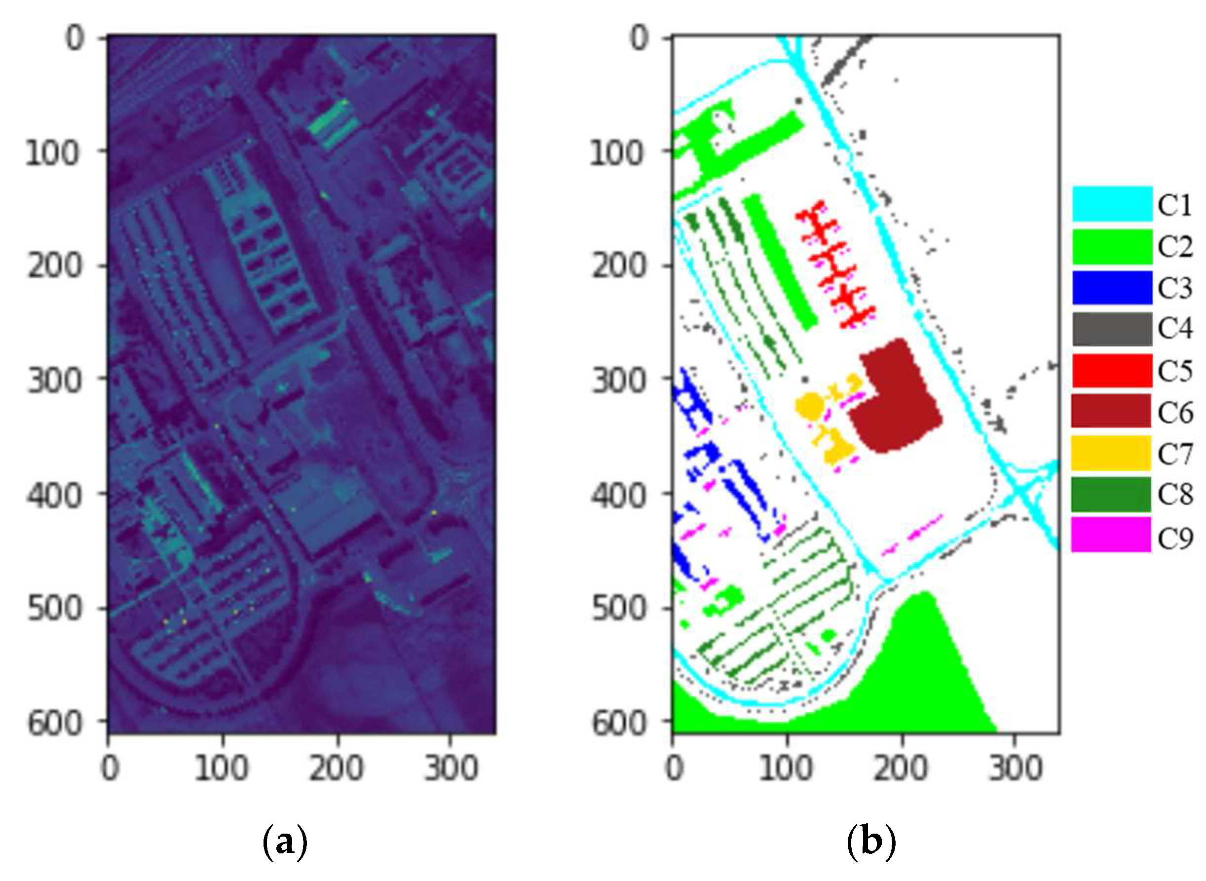
(3) Experimental Results on the Pavia University Dataset

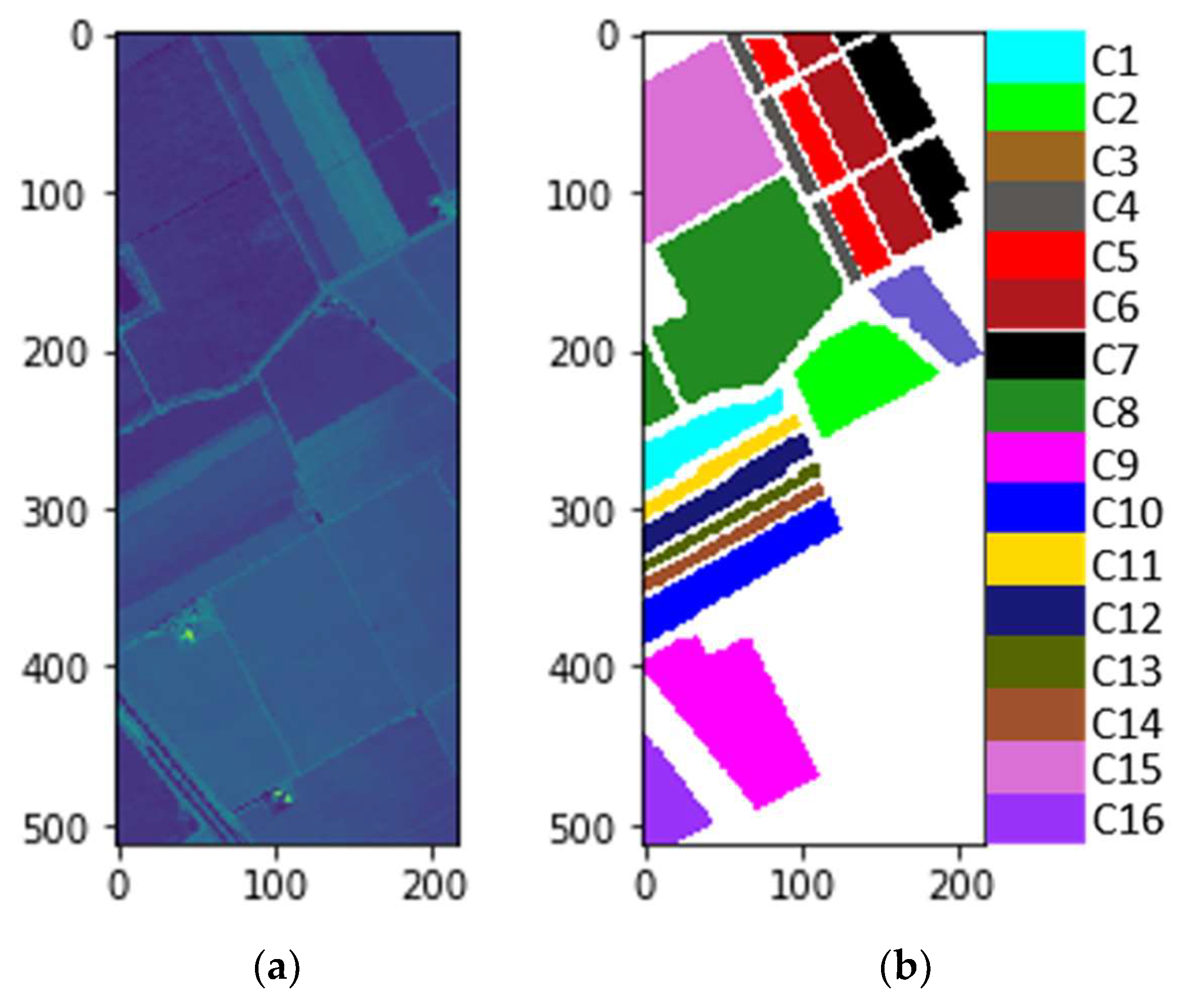
To demonstrate the relationship between classification accuracies and inter-class separability,

Table 6. The details of classification results for Pavia University data.

	C1	C2	C3	C4	C5	C6	C7	C8	C9
C1	4790	0	31	0	2	1	108	70	2
C2	6	13,871	2	58	0	169	0	7	0
C3	29	1	1341	0	0	0	1	179	0
C4	1	42	0	2172	0	2	0	0	0
C5	1	0	0	0	1011	0	0	0	0
C6	12	150	0	3	1	3580	0	10	0
C7	60	0	1	0	0	0	887	2	0
C8	64	2	212	0	0	7	0	2478	0
C9	0	0	0	0	0	0	0	0	716

and

Table 7. The detailed classification accuracy of all the classes for Pavia University data.

	C1	C2	C3	C4	C5	C6	C7	C8	C9
C1	95.72%	0.00%	0.62%	0.00%	0.04%	0.02%	2.16%	1.40%	0.04%
C2	0.04%	98.29%	0.01%	0.41%	0.00%	1.20%	0.00%	0.05%	0.00%
C3	1.87%	0.06%	86.46%	0.00%	0.00%	0.00%	0.06%	11.54%	0.00%
C4	0.05%	1.89%	0.00%	97.97%	0.00%	0.09%	0.00%	0.00%	0.00%
C5	0.10%	0.00%	0.00%	0.00%	99.90%	0.00%	0.00%	0.00%	0.00%
C6	0.32%	3.99%	0.00%	0.08%	0.03%	95.31%	0.00%	0.27%	0.00%
C7	6.32%	0.00%	0.11%	0.00%	0.00%	0.00%	93.37%	0.21%	0.00%
C8	2.32%	0.07%	7.67%	0.00%	0.00%	0.25%	0.00%	89.69%	0.00%
C9	0.00%	0.00%	0.00%	0.00%	0.00%	0.00%	0.00%	0.00%	100.00%

display the details of the classification results for Pavia University data at nc_layer = 2 and g = 20. In Table 6, the value in the ith row, jth column means the number of samples of the jth class which is classified to the ith class. Each row represents the samples in a predicted class, and each class represents the samples in an actual class. The values on diagonal line means the number of samples which are classified correctly. Those values not on diagonal line means false positives or false negatives. For example, in the first row, 4790 samples of C1 are classified correctly, while 31 samples of C3 are misclassified into C1, which means false positives. In the seventh column, 887 samples of C7 are classified correctly, while 108 samples are misclassified into C1, which means false negatives.

In Table 7, the value in the ith row, jth column means the percentage of the samples classified into the ith class from the jth class. The values on diagonal line are just the classification accuracies of corresponding classes. For example, 93.37% of C7 samples are classified correctly, but 6.32% of the samples classified into C7 are from C1, which are misclassified. The smaller the difference of mean spectral curves, the smaller the difference among spectral feature maps from a different class, the worse the inter-class separability, the easier it is to cause misclassification. As shown in Figure 12, the curves of C3 and C8 are very similar, that is, the difference between C3 and C8 is small. So, many samples (212) of C3 are misclassified into C8. Similarly, many samples (179) of C8 are misclassified into C3. In this way, it is not difficult to explain that the OA of proposed method is only 89.95% on the Indian Pines dataset, while 96.01% on the Salinas dataset and 96.15% on the Pavia University dataset. Because at many bands, there is serious aliasing in the spectral mean curves of the Indian Pines dataset (Figure 4), which means poor inter-class separability. Therefore, there exist serious misclassification in some classes, resulting in the decline of overall classification accuracy for the Indian Pines dataset.

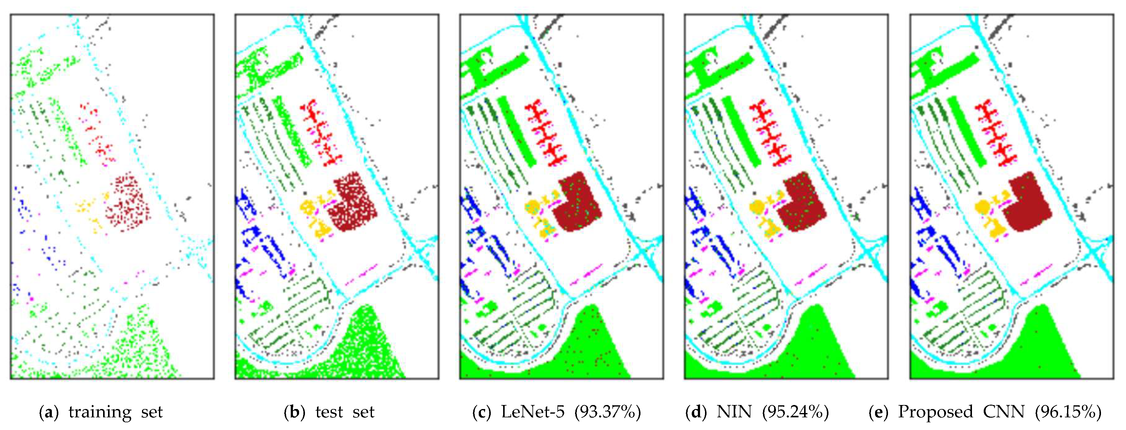
(4) Comparison with Other Methods

In order to further evaluate the effectiveness of the proposed method, we implement two classical CNN architectures, NIN and LeNet-5. We take nc_layer = 2 and g = 20, the architectures of which are shown in

Table 8. The architecture of proposed CNN/NIN/LeNet-5.

Layer	Output Size	Proposed CNN	NIN	LeNet-5
Conv	14 × 14	$\left[\begin{array}{cc}3\times 3,& 40\\ 3\times 3,& 40\\ 3\times 3,& 40\\ 1\times 1,& 40\\ 1\times 1,& 40\end{array}\right]$	$\left[\begin{array}{cc}3\times 3,& 40\\ 3\times 3,& 40\\ 3\times 3,& 40\\ 1\times 1,& 40\\ 1\times 1,& 40\end{array}\right]$	$\left[\begin{array}{cc}5\times 5,& 6\end{array}\right]$
Pool	7 × 7	3 × 3 max pool, stride 2
Conv	7 × 7	$\left[\begin{array}{cc}1\times 1,& 80\\ 3\times 3,& 80\\ 1\times 1,& 80\\ 3\times 3,& 80\\ 1\times 1,& 40\end{array}\right]$	$\left[\begin{array}{cc}3\times 3,& 80\\ 3\times 3,& 80\\ 3\times 3,& 80\\ 1\times 1,& 80\\ 1\times 1,& 40\end{array}\right]$	$\left[\begin{array}{cc}5\times 5,& 16\end{array}\right]$
Pool	3 × 3	2 × 2 average pool, stride 2
Classification	1 × 1	global average pool		120-D FC, 84-D FC
		16-D FC, Softmax
FLOPS		12,693,600	13,869,600	175,704

. The classification results on three datasets are shown in

Table 9. Classification results of different CNN architectures on three HSI datasets.

Dataset	Index	LeNet-5	NIN	Proposed CNN
Indian Pines	OA	85.78%	88.97%	89.95%
	AA	85.33%	86.36%	90.92%
	Kappa	0.8379	0.8742	0.8845
Salinas	OA	94.28%	95.09%	96.01%
	AA	97.38%	97.94%	98.11%
	Kappa	0.9363	0.9453	0.9555
Pavia University	OA	93.37%	95.24%	96.15%
	AA	92.12%	94.58%	95.19%
	Kappa	0.9120	0.9359	0.9488

.

Table 10. Computing consumption of different CNN architectures on the Indian Pines dataset.

Methods	Training Time	Testing Time	OA
LeNet-5	74 s	5.37 s	85.78%
NIN	174.36 s	27.68 s	88.97%
Proposed CNN	131.53 s	24.39 s	89.95%

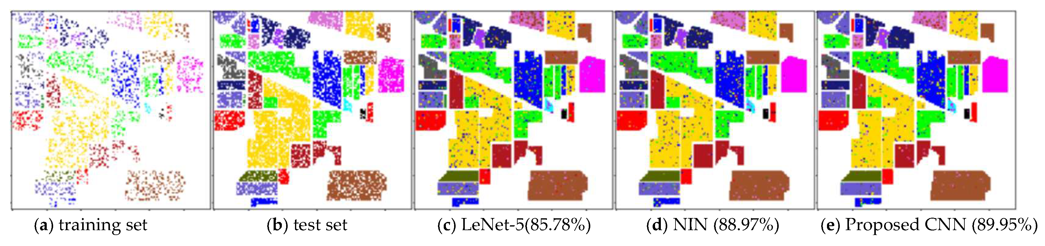
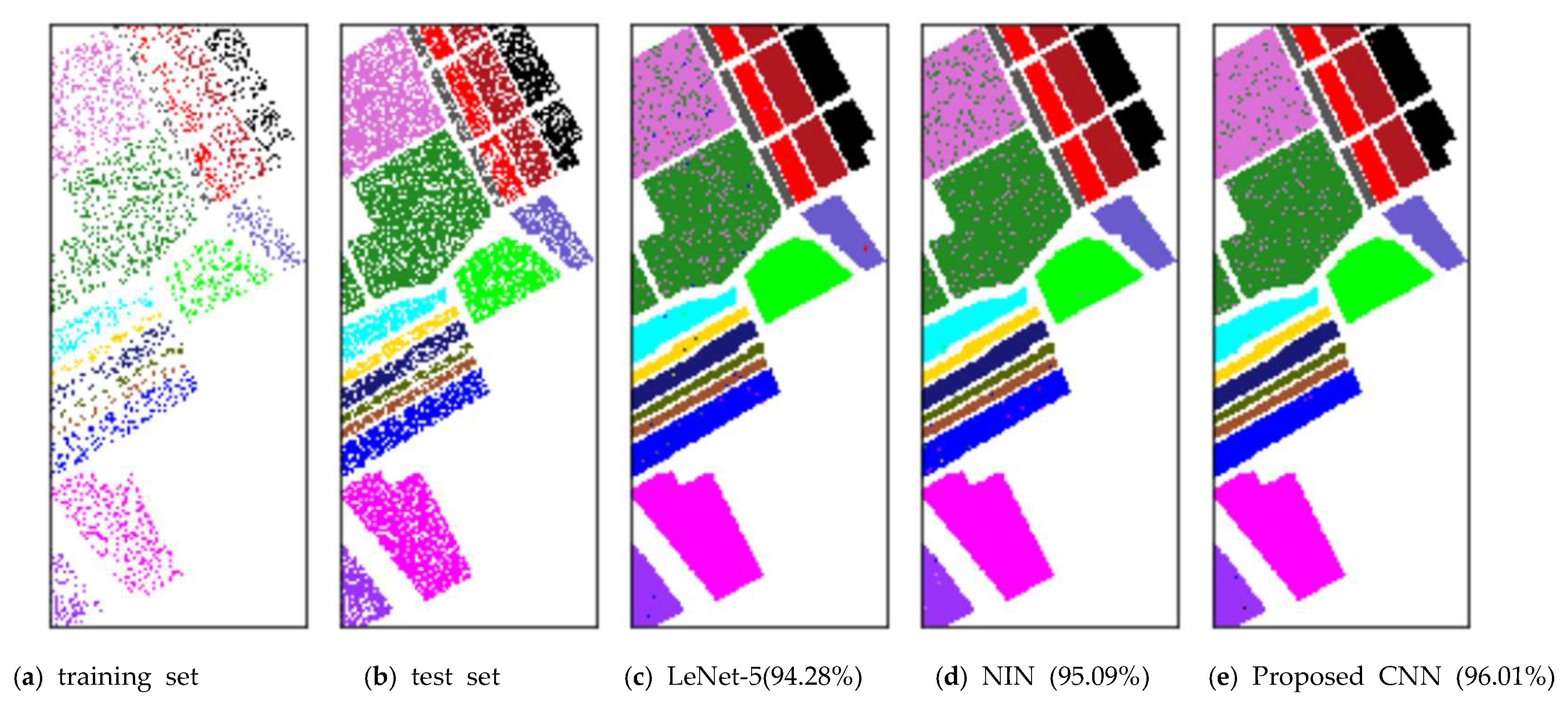
displays the total run time for training and testing on the Indian Pines dataset classification, respectively. Figure 15, Figure 16 and Figure 17 display the corresponding classification maps. It is easy to know that the classification performance of the proposed method is better than all the comparison methods. Furthermore, as can be seen from Table 8 and Table 10, the FLOPS (floating-point operations) of proposed CNN is 10⁶ less than that of NIN, and the training time and testing time in Indian Pines data classification are also significantly less than that of NIN. The OA of the proposed CNN is 0.98% more than that of NIN, which demonstrates the effectiveness of the ASC–FR module. However, FLOPS and computing consumption of LeNet-5 are much less than that of proposed CNN and NIN. Its shallow structure and insufficient training samples of HSI severely restrict the classification performance of LeNet-5. As a result, the OA of LeNet-5 is 3.19% less than that of NIN, and 4.17% less than that of proposed CNN.

Finally, the classification performance of the proposed method is compared with some other HSI classification methods, as shown in

Table 11. Comparison with other methods for the Indian Pines dataset.

References	Baseline	Feature	Training Set	Accuracy
Hu et al. [19]	CNN	Spectral	8 classes, 200 samples per class	90.16% (90.74%)
Chen et al. [17]	CNN	Spectral	150 samples per class	87.81% (88.16%)
Chen et al. [32]	DBN	Spectral–Spatial	50%	91.34% (92.58%)
Fu et al. [33]	DAE	Spectral	30%	89.82% (90.18%)
Sun et al. [5]	BWSVM	Spectral	25%	88% (89.95%)
Li et al. [6]	KELM	Spectral	10%	80.37% (84.53%)
Li et al. [6]	KSVM	Spectral	10%	79.17% (84.53%)
Wei et al. [7]	FPCA+KELM	Spectral	15%	87.62% (87.92%)
Hu et al. [19]	RBF-SVM	Spectral	8 classes, 200 samples per class	87.60% (90.74%)

. In this table, the accuracies outside brackets are taken from corresponding references directly, and those accuracies in brackets are obtained by the proposed method. It should be noted that we obtain the classification accuracy by dividing the training set and the test set according to the corresponding reference. The table demonstrates that the classification performance of proposed method outperforms all the comparison methods. In addition, DBN means deep belief network and DAE means denoising autoencoders in Table 11.

5. Conclusions

In this work, an HSI classification method based on ASC–FR is proposed. In data pre-processing, each 1D spectral vector that corresponds to a labeled pixel is transformed into a 2D spectral feature map, thereby highlighting the differences among samples and weakening the influence of strong correlation among bands for HSI classification. In the CNN design, 1 × 1 convolution layers are adopted to reduce the network parameters and increase network complexity, thus extracting increasingly accurate hyperspectral data features. Through the ASC–FR module, the utilization rate of the high-dimensional features in the network can be improved, the features of hyperspectral data can be extracted meticulously and comprehensively, overfitting can be prevented to a certain extent, and classification accuracy can be improved. Overlapping pooling and GAP are used to integrate the data features, thereby greatly enhancing the learning capability of the network for spectral features and improving the generalization capability of the CNN. Experimental results show when only 25% samples are selected for the training set, the classification accuracy of the proposed method can reach 89.95% for the Indian Pines dataset, and even 96.01% for the Salinas dataset and 96.15% for the Pavia University dataset. Comparative experiments on three benchmark HSI datasets demonstrate that the proposed ASC–FR module can improve the classification accuracy of CNNs for HSIs effectively and the proposed classification method has excellent classification performance, which outperforms all the comparison methods. However, the proposed method only configures the number of channels in each convolution layer simply, there is still much room for improvement. Furthermore, the spatial information of hyperspectral images cannot be effectively utilized by the proposed method. In future work, we will optimize the combination of convolution layer channels through a large number of experiments, and adopt some approaches to augment the number of training samples, more importantly, combining spectral information and spatial information to achieve hyperspectral classification. Finally, we plan to optimize the network structure of the proposed method by referring to the latest progress in CNN research. In those ways, we believe the performance of CNN-based HSI classification under a small training set can be improved effectively and significantly.

References

1. Hughes, G. On the mean accuracy of statistical pattern recognizers. IEEE Trans. Inf. Theory 1968, 14, 55–63. [Google Scholar] [CrossRef]
2. Tong, Q.; Zhang, B.; Zheng, L. Hyperspectral Remote Sensing—Principle, Technology and Application; Higher Education Press: Beijing, China, 2006. [Google Scholar]
3. Wang, M.; Gao, K.; Wang, L.J.; Miu, X.H. A Novel Hyperspectral Classification Method Based on C5.0 Decision Tree of Multiple Combined Classifiers. In Proceedings of the Fourth International Conference on Computational and Information Sciences, Chongqing, China, 17–19 August 2012; pp. 373–376. [Google Scholar]
4. Rojas-Moraleda, R.; Valous, N.A.; Gowen, A.; Esquerre, C.; Härtel, S.; Salinas, L.; O’Donnell, C. A frame-based ANN for classification of hyperspectral images: Assessment of mechanical damage in mushrooms. Neural Comput. Appl. 2017, 28, 969–981. [Google Scholar] [CrossRef]
5. Sun, W.; Liu, C.; Xu, Y.; Tian, L.; Li, W.Y. A Band-Weighted Support Vector Machine Method for Hyperspectral Imagery Classification. IEEE Geosci. Remote Sens. Lett. 2017, 14, 1710–1714. [Google Scholar] [CrossRef]
6. Li, J.; Du, Q.; Li, W.; Li, Y.S. Optimizing extreme learning machine for hyperspectral image classification. J. Appl. Remote Sens. 2015, 9, 097296. [Google Scholar] [CrossRef]
7. Wei, Y.; Xiao, G.; Deng, H.; Chen, H.; Tong, M.G.; Zhao, G.; Liu, Q.T. Hyperspectral image classification using FPCA-based kernel extreme learning machine. Optik Int. J. Light Electron Opt. 2015, 126, 3942–3948. [Google Scholar] [CrossRef]
8. Zhang, X.; Zhou, X.; Lin, M.; Sun, J. ShuffleNet: An Extremely Efficient Convolutional Neural Network for Mobile Devices. arXiv, 2017; arXiv:1707.01083v2. [Google Scholar]
9. Shrivastava, A.; Sukthankar, R.; Malik, J.; Gupta, A. Beyond Skip Connections: Top-Down Modulation for Object Detection. arXiv, 2016; arXiv:1612.06851. [Google Scholar]
10. Dai, J.F.; Qi, H.Z.; Xiong, Y.W.; Li, Y.; Zhang, G.D.; Hu, H.; Wei, Y.C. Deformable Convolutional Networks. In Proceedings of the IEEE International Conference on Computer Vision, Venice, Italy, 22–29 October 2017; pp. 764–773. [Google Scholar]
11. Yann, L.; Leon, B.; Yoshua, B.; Patrick, H. Gradient-based learning applied to document recognition. Proc. IEEE 1998, 86, 2278–2324. [Google Scholar] [Green Version]
12. Krizhevsky, A.; Sutskever, I.; Hinton, G.E. ImageNet classification with deep convolutional neural networks. In Proceedings of the International Conference on Neural Information Processing Systems, Lake Tahoe, NV, USA, 3–6 December 2012; pp. 1097–1105. [Google Scholar]
13. Lin, M.; Chen, Q.; Yan, S. Network in Network. arXiv, 2014; arXiv:1312.4400v3. [Google Scholar]
14. Szegedy, C.; Liu, W.; Jia, Y.Q.; Sermanet, P.; Reed, S.; Anguelov, D.; Erhan, D.; Vanhoucke, V.; Rabinovich, A. Going Deeper with Convolutions. In Proceedings of the IEEE Conference on Computer Vision and Pattern Recognition, Boston, MA, USA, 7–12 June 2015; pp. 1–9. [Google Scholar]
15. Sun, Y.; Wang, X.; Tang, X. Deeply learned face representations are sparse, selective, and robust. In Proceedings of the IEEE Conference on Computer Vision and Pattern Recognition, Boston, MA, USA, 7–12 June 2015; pp. 2892–2900. [Google Scholar]
16. He, K.M.; Zhang, X.Y.; Ren, S.Q.; Sun, J. Deep Residual Learning for Image Recognition. In Proceedings of the Computer Vision and Pattern Recognition, Las Vegas, NV, USA, 27–30 June 2016; pp. 770–778. [Google Scholar]
17. Chen, Y.S.; Jiang, H.L.; Li, C.Y.; Jia, X.P. Deep Feature Extraction and Classification of Hyperspectral Images Based on Convolutional Neural Networks. IEEE Trans. Geosci. Remote Sens. 2016, 54, 6232–6251. [Google Scholar] [CrossRef]
18. Yue, Q.; Ma, C. Deep Learning for Hyperspectral Data Classification through Exponential Momentum Deep Convolution Neural Networks. J. Sens. 2016, 2016, 3150632. [Google Scholar] [CrossRef]
19. Hu, W.; Huang, Y.Y.; Wei, L.; Zhang, F.; Li, H.C. Deep Convolutional Neural Networks for Hyperspectral Image Classification. J. Sens. 2015, 2015, 258619. [Google Scholar] [CrossRef]
20. Lee, H.; Kwon, H. Going Deeper with Contextual CNN for Hyperspectral Image Classification. IEEE Trans. Image Process. 2017, 26, 4843–4855. [Google Scholar] [CrossRef] [PubMed]
21. Lee, H.; Kwon, H. Contextual deep CNN based hyperspectral classification. In Proceedings of the Geoscience and Remote Sensing Symposium, Beijing, China, 10–15 July 2016. [Google Scholar]
22. Li, Y.; Zhang, H.; Shen, Q. Spectral-Spatial Classification of Hyperspectral Imagery with 3D Convolutional Neural Network. Remote Sens. 2017, 9, 67. [Google Scholar] [CrossRef]
23. Makantasis, K.; Karantzalos, K.; Doulamis, A.; Doulamis, N. Deep supervised learning for hyperspectral data classification through convolutional neural networks. In Proceedings of the 2015 IEEE International Geoscience and Remote Sensing Symposium (IGARSS), Milan, Italy, 26–31 July 2015; pp. 4959–4962. [Google Scholar]
24. Simonyan, K.; Zisserman, A. Very Deep Convolutional Networks for Large-Scale Image Recognition. arXiv, 2014; arXiv:1409.1556. [Google Scholar]
25. Alam, F.I.; Zhou, J.; Liew, W.C.; Jia, X.P. CRF learning with CNN features for hyperspectral image segmentation. In Proceedings of the Geoscience and Remote Sensing Symposium, Beijing, China, 10–15 July 2016; pp. 6890–6893. [Google Scholar]
26. Yuan, Q.Q.; Zhang, Q.; Li, J.; Shen, H.F.; Zhang, L.P. Hyperspectral Image Denoising Employing a Spatial-Spectral Deep Residual Convolutional Neural Network. arXiv, 2018; arXiv:1806.00183. [Google Scholar]
27. Liu, Q.S.; Hang, R.L.; Song, H.H.; Zhu, F.P.; Plaza, J.; Plaza, A. Adaptive Deep Pyramid Matching for Remote Sensing Scene Classification. arXiv, 2016; arXiv:1611.03589v1. [Google Scholar]
28. Yu, S.; Jia, S.; Xu, C. Convolutional neural networks for hyperspectral image classification. Neurocomputing 2016, 219, 88–98. [Google Scholar] [CrossRef]
29. Makantasis, K.; Doulamis, A.D.; Doulamis, N.D.; Nikitakis, A. Tensor-Based Classification Models for Hyperspectral Data Analysis. IEEE Trans. Geosci. Remote Sens. 2018, 99, 1–15. [Google Scholar] [CrossRef]
30. Chen, Y.S.; Zhu, L.; Ghamisi, P.; Jia, X.P.; Li, G.Y.; Tang, L. Hyperspectral Images Classification with Gabor Filtering and Convolutional Neural Network. IEEE Geosci. Remote Sens. Lett. 2017, 14, 2355–2359. [Google Scholar] [CrossRef]
31. He, K.M.; Zhang, X.Y.; Ren, S.Q.; Sun, J. Delving Deep into Rectifiers: Surpassing Human-Level Performance on ImageNet Classification. In Proceedings of the IEEE International Conference on Computer Vision, Santiago, Chile, 7–13 December 2015; pp. 1026–1034. [Google Scholar]
32. Chen, Y.; Zhao, X.; Jia, X. Spectral–Spatial Classification of Hyperspectral Data Based on Deep Belief Network. IEEE J. Sel. Top. Appl. Earth Obs. Remote Sens. 2015, 8, 2381–2392. [Google Scholar] [CrossRef]
33. Fu, Q.Y.; Yu, X.C.; Tan, X.; Wei, X.P.; Zhao, J.L. Classification of Hyperspectral Imagery Based on Denoising Autoencoders. J. Geomat. Sci. Technol. 2016, 33, 485–489. [Google Scholar]
Figure 1. The diagram of data pre-processing procedure.
Ijgi 07 00349 g001
Figure 2. Proposed convolutional neural network (CNN) architecture.
Ijgi 07 00349 g002
Figure 3. The Indian Pines image: (a) the 21th band image; (b) the ground truth of Indian Pines, where the white area represents the unlabeled pixels.
Ijgi 07 00349 g003
Figure 4. Mean spectral signatures of 16 classes in the Indian Pines dataset.
Ijgi 07 00349 g004
Figure 5. 2D spectral feature maps of 16 classes in the Indian Pines dataset.
Ijgi 07 00349 g005
Figure 6. The Salinas image: (a) the 21th band image; (b) the ground truth of Salinas, where the white area represents the unlabeled pixels.
Ijgi 07 00349 g006
Figure 7. Mean spectral signatures of 16 classes in the Salinas dataset.
Ijgi 07 00349 g007
Figure 8. 2D spectral feature maps of 16 classes in the Salinas dataset.
Ijgi 07 00349 g008
Figure 9. The Pavia University image: (a) the 21th band image; (b) the ground truth of Salinas, where the white area represents the unlabeled pixels.
Ijgi 07 00349 g009
Figure 10. Mean spectral signatures of 16 classes in the Pavia University dataset.
Ijgi 07 00349 g010
Figure 11. 2D spectral feature maps of 16 classes in the Pavia University dataset.
Ijgi 07 00349 g011
Figure 12. Classification result of proposed method when nc_layer = 2, g = 8/20/32: (a) shows the classification accuracy per class, (b) shows overall accuracy/average accuracy/kappa coefficient (OA/AA/Kappa).
Ijgi 07 00349 g012
Figure 13. Classification results of proposed method nc_layer = 2, g = 8/20/32: (a) shows the classification accuracy per class, (b) shows the OA/AA/Kappa.
Ijgi 07 00349 g013
Figure 14. Spectral curves of 100 bands and 144 bands in the Indian Pines dataset.
Ijgi 07 00349 g014
Figure 15. Classification maps of different CNN architectures on the Indian Pines dataset.
Ijgi 07 00349 g015
Figure 16. Classification maps of different CNN architectures on the Salinas dataset.
Ijgi 07 00349 g016
Figure 17. Classification maps of different CNN architectures on the Pavia University dataset.
Ijgi 07 00349 g017