Susceptibility to Translational Slide-Type Landslides: Applicability of the Main Scarp Upper Edge as a Dependent Variable Representation by Reduced Chi-Square Analysis

Abstract

The applicability of main scarp upper edge (MSUE) as dependent variable representation was performed in a translational slide susceptibility zonation of the Milia and Roglio basins, Italy. Two landslide inventories were built thanks to detailed geomorphological mapping and aerial photograph analysis. The landslides were used to create the models before 1975, while those after 1975 were employed to validate the predictive power of the model. Possible landslide-related factors were chosen from a geomorphological survey. The inventory landslide maps and the landslide-related factor maps were processed by conditional analysis, producing landslide susceptibility maps with five susceptibility classes. A comparison between the distribution of landslides after 1975 and those derived from models provided the predictive power of each model, which in turn was used to define the best predictive model. Reduced chi-square analysis allowed to define the efficiency of MSUE as dependent variable representation. MSUE can be applied as dependent variable representation to landslide susceptibility zonation with appreciable results. In the Roglio basin, slope angle, distance from streams, and from tectonic lineaments proved to be the main controlling factors of translational slides, whereas in the Milia basin, lithology and slope angle gave more satisfactory results as landslide-predisposing factors.

1. Introduction

If only social and economic parameters are considered when planning urban and industrial growth, the derived infrastructures (e.g., buildings, roads, factories) may be threatened by natural phenomena, such as those of a geomorphological nature. As a matter of fact, processes like landsliding and flooding can cause severe damages and, in many cases, lead to the loss of human lives. The use of maps able to depict the spatial distribution of a natural hazard or susceptibility to its occurrence has become crucial for correct territorial planning, risk mitigation and management [1,2]. In this regard, how to generate maps of landslide susceptibility is a key question, since landsliding is one of the most common sources of natural risk.

Landslide susceptibility (LS) is the spatial probability of landslide occurrence [3] and differs from landslide hazard, since it provides no information on the timing and magnitude of predicted landslides. However, landslide susceptibility is the first step in landslide risk assessment [3,4,5,6,7,8].

Statistical methods are the most commonly used techniques to assess landslide susceptibility over medium- and large-scale areas [9,10,11,12,13].

All statistical methods are based on the common assumption that landslides are more likely to occur in areas where boundary conditions are similar to areas in which landslides have occurred [14]; however, they necessarily require the knowledge of the factor conditions existing before the landslide occurrence. With the exception of very recent landslides, the morphometric factor maps available (e.g., slope angle) represent the post-landsliding condition. Therefore, in most cases it is necessary to identify the morphometric factor conditions before the landslides.

The authors who have studied at the problem agree that the pre-landslide conditions may be similar to those found in an external neighborhood of the landslide source area [15,16,17,18,19].

Among the systems of landslide representations that have been applied with notable results, the main scarp upper edge method (MSUE-Method) [10] allows for easier automatic research of the factor values in the undisturbed belt external to the rupture zone of the landslide [10,20].

The applicability of the MSUE, however, has been poorly studied. The predictive ability of MSUE models has been analyzed previously by a validation dataset generated using a random split method for observed landslides. If the landslides used in the model validation dataset also require the pre-landslide conditions to be reconstructed, the LS image used to define the maximum likelihood in the model could not represent the real LS, owing to the degree of subjectivity used in the reconstruction process. The best predictive model chosen from the validation procedure may poorly predict future landslides. In this case, following the procedures described in previous studies [12,21,22,23], the forecasting model should be implemented by an older landslide inventory, and more recent landslides should be exploited to evaluate the prediction.

This study represents an attempt to analyze the applicability of MSUE as dependent variable representation. For the final purpose of this study, the conditional analysis method has been applied to factor combinations [24], as it has fewer limitations than other systems of statistical analysis. In particular, this method does not require independence variables and covariate normal distribution.

To achieve the study goal rigorously, it was also necessary to perform the surveys in two different basins by means of two landslide inventories related to a period preceding and another succeeding a fixed date. More specifically, the model validation procedure was based on the “wait and see” concept [25], according to which, in the spatial database, it was assumed that the time of the study was the year 1975 and that all the spatial data available in 1975 had been compiled, including the distribution of the MSUEs of the landslides prior to that year. Consequently, the landslides related to a period before 1975 were used to create the models, while those related to a period later than 1975 were used to validate the predictive power of the models. Finally, an analysis of reduced chi-square was performed to define the efficiency of MSUE as a dependent variable.

2. Geography

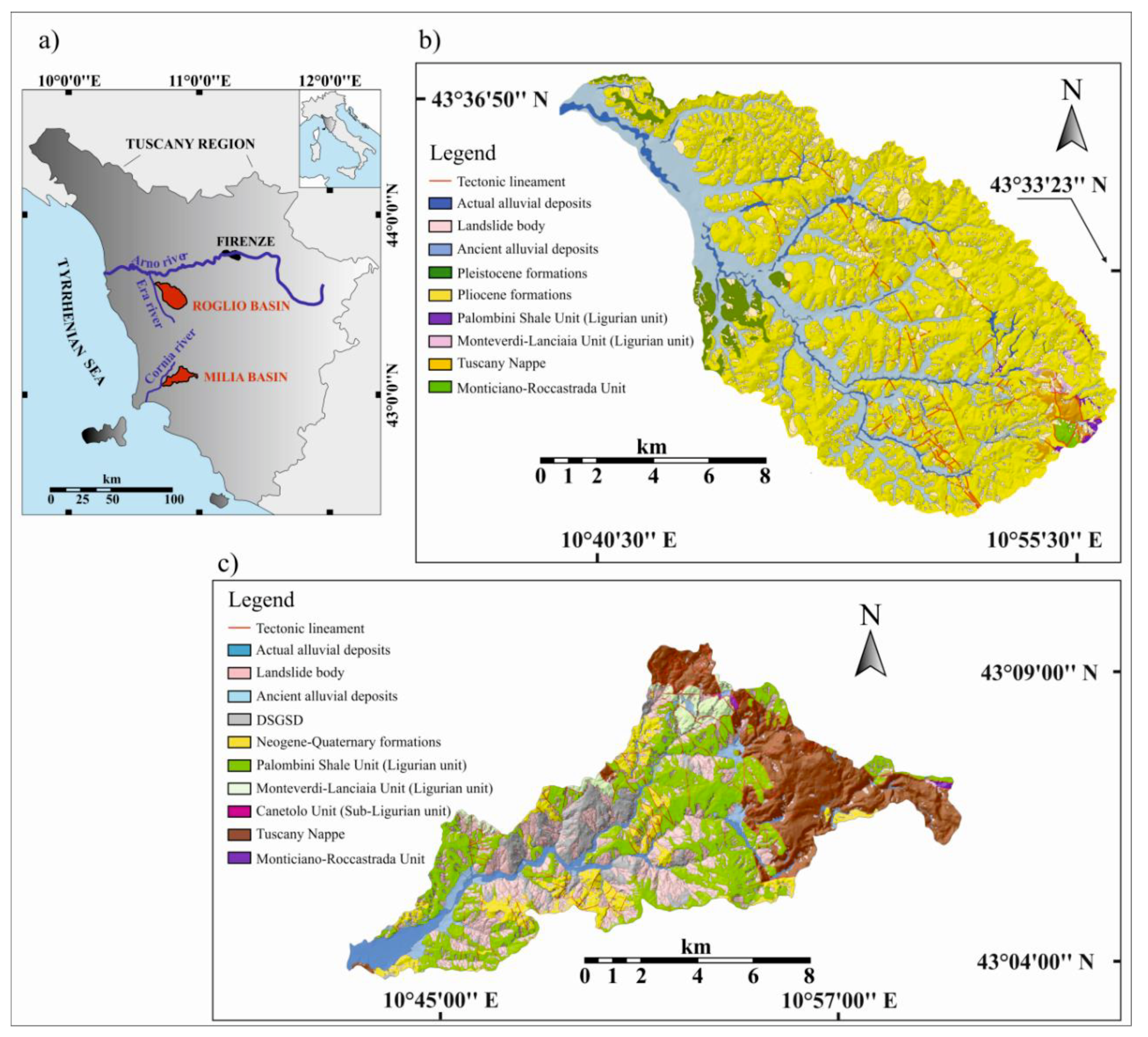
The study areas were the Milia and Roglio basins, situated in southern-central and central Tuscany (Italy), respectively (Figure 1).

The Milia basin has an extension of 101 km² and an elevation ranging from 39 m to 913 m asl, with an average elevation of 336 m (standard deviation = 167.5 m), whereas the catchment area of the Roglio River covers 160 km² with an elevation ranging from 20 m to 500 m asl, with an average of 130.9 m (standard deviation = 72.1 m). The basins have a predominantly hilly morphology, generally with not very steep slopes; the connection areas between the valley floor and the slopes are very extended. In the studied basins, most of the streams show strong vertical and lateral erosion tendencies.

3. Geology and Geomorphology

A complex sheet stack of Ligurian and Sub-Ligurian units emplaced above the Tuscan Nappe is the result of the compressional events that characterized the Apennine tectonic history [26,27]. The units of the Ligurian Domain are representative of distal turbiditic and pelagic environments and of the oceanic crust that formed the ancient Ligurian-Piedmont Basin, while the Tuscany units are mostly represented by the Mesozoic carbonate succession associated with very few outcrops of the cretaceous-tertiary turbiditic and hemipelagic sequence. The Tuscany units are overthrusted above the Monticiano-Roccastrada Unit (Tuscany Autochthonous Metamorphic Unit), which is characterized by an alternation of phyllites, marbles and quartzite lithotypes. On the whole, four major rock and sediment types are present in each basin: (i) marine and continental sediments made up of clay, marly clay, sand, gravel and gravelly sand, (ii) flysch deposits, comprising layered sandstone, marly limestone, and shale, (iii) carbonate rocks, comprising layered and massive limestone, and (iv) metamorphic rocks, made up of quartzite and slate. The Palombini Shale Unit (Ligurian unit) mainly characterizes the Milia basin, instead marine and continental sediments (Pliocene formations) are the most extensive outcrops in the Roglio basin (Figure 1). Each basin experienced an extensional tectonics that highly controlled the post-collisional evolution of this part of the Apennines. This tectonic style began at the end of the Early Miocene [28]. Since the Middle Pleistocene differential uplift, lowering and tilting phenomena of mountain sectors have caused a rapid incision of the hydrographic networks, promoting the formation of several fluvial terraces along both basins.

Translational slides, rotational slides, and flows [29] dominate the morphology of the studied basins. In addition, many Deep-Seated Gravitational Slope Deformations (DSGSDs, [30]) have been identified in the Milia basin. Their occurrence can be related to the Pleistocene tectonics and to the lowering of the local fluvial base level. A Sackung type [31] can be proposed with regard to the movement. 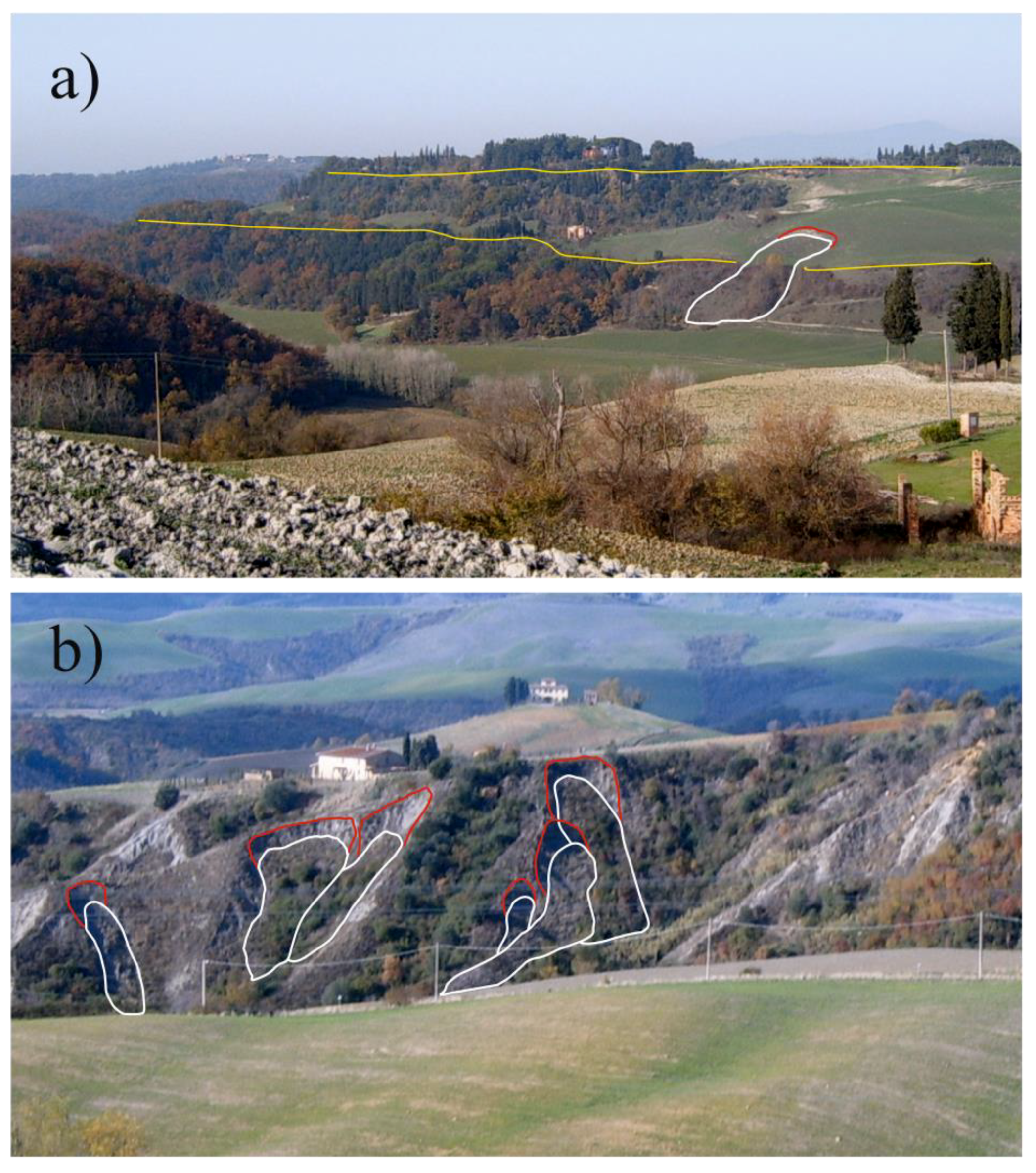According to the authors [32], DSGSDs in the Milia basin played a significant role as landslide-predisposing factor. The presence of clayey and clayey-sandy lithologies in the Roglio basin has promoted the development of badlands and “balze” morphologies. “Balzes” [33] are constituted by a series of degradation scarps, which interrupt the continuity of the slope profile where an alternation of sandy and clay layers has occurred (Figure 2a). The numerous badlands and “balze” morphologies, whose genesis can be correlated to the rainwater erosive action on the Pliocene deposits, are currently affected by slope processes mainly connected with the development of landslides (Figure 2b).

Many translational slides have developed from the bodies of older landslides in both basins.

4. Basic Theory, Database Building and Procedures for LS Zonation

4.1. MSUE-Conditional Analysis Method

The conditional analysis method applied to factor combinations [24] is based on Bayes’ Theorem [34] for which the likelihood of landslide occurrences conditioned by the occurrence of different combinations of environmental factors (conditioning events) can be defined by computing the landslide density within each different conditioning event (Unique Condition Unit, UCU) [14]. More specifically, the method considers a number of environmental factors, thought to be strictly connected with landslide occurrence. The data layers, where each factor is subdivided into classes, are crossed to obtain all possible factor combinations (UCU-maps). For each of these factor combinations, landslide density is then quantified within each UCU by crossing the relative UCU-map with the landslides chosen as model training dataset. Considering that landslide density is assumed to be equivalent to the future landslide probability at a specific UCU [14], from this process we obtain a number of LS models equal to the number of possible factor combinations. The best model is chosen by comparing the distribution of landslides used as validation dataset and of those derived from the models. This method tends to assess the most suitable combination for defining the LS zonation with the highest predictive ability.

In this study the landslides have been identified by the MSUEs. Consequently, to consider the UCUs present in the external neighborhood of the landslide source area (which could be representative of the geo-environmental conditions existing before the development of landslides), an upstream 10 m buffer of is used for each MSUE. This buffer extension is the highest threshold value for which we can avoid the buffer areas passing over the divide line.

Therefore, the method applied to the LS zonation of the Milia and Roglio basins assumes the conditional probability of landslide occurrence for a given UCU as the ratio between the MSUE buffer area affecting UCU and the area of UCU [19].

4.2. Landslide Dataset

Geological and geomorphological field surveys were conducted using the Tuscany Region topographic maps (scale 1:10,000) and the Tuscany Region orthophotos (1 m ground-sample-distance ortho-imagery rectified to a horizontal accuracy of within ±4 m) dating back to 2006 and 2003 for the Milia and Roglio basins, respectively. A geomorphological field survey was also carried out with the aid of GPS point acquisition (accuracy ≤3 m, precision ≤1 m) and of the stereoscopic interpretation of 1975 aerial photographs (flight EIRA75).

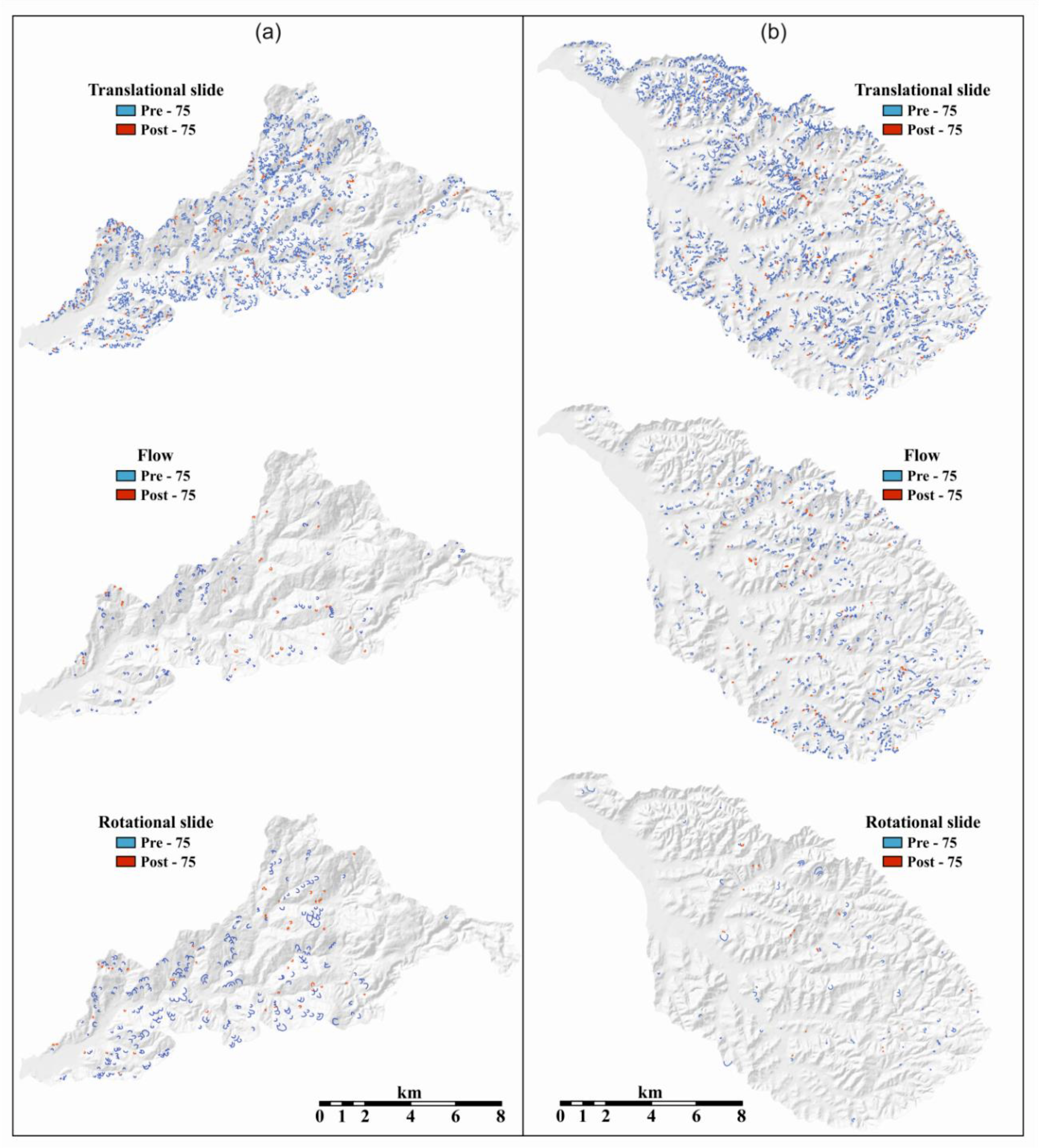
The landslides of each basin were split into two temporal groups by stereoscopic analysis of the aerial photographs relating to 1975 (Figure 3). The landslides that occurred before 1975 were used as a model training set, whereas the landslides that occurred after 1975 have been used as a model validation set. In agreement with Guzzetti et al. [5], LS analysis should be performed for different types of landslides. For this reason, the landslides were grouped into separate datasets based on movement typology. Following the division proposed by Keefer [35], we only considered deep-seated (≥3 m) landslides in order to avoid the introduction of shallow and easily degradable landslides into the model validation dataset.

A total of 2039 landslides were identified in the Milia basin (Figure 3a). The landslides covered a surface of about 22.6 km², representing 22.4% of the whole basin area. On the basis of the observations made during the field work, these 2039 landslides were divided into three typologies: translational slide (1577), flow (155), and rotational slide (307). Among these, 128 translational slides, 31 flow and 46 rotational slides have occurred since 1975.

In the Roglio basin a total of 4137 deep-seated landslides were identified, which occupied a surface of about 20.7 km², representing 12.5% of the whole basin area. The landslides were classified into three typologies: translational slide (3174), flow (873), and rotational slide (90). Among these, 233 translational slides, 109 flow and 19 rotational slides have occurred since 1975 (Figure 3b).

Overall, the studied basins were affected mainly by translational slide-type landslides. The aim of this study was to analyze the applicability of MSUE as dependent variable representation by using a statistical approach. For this reason, only the translational slides were used for analysis, to ensure that the predictive model could be adequately trained because of the abundance of landslides.

For each basin, the maps of the MSUEs relative to the training and validation datasets were obtained from the geomorphological maps previously digitized in ArcGIS (MSUEs pre- and post-1975). The maps of the buffers were achieved in polygonal vector format from the MSUE maps by using the ArcInfo 9.2 (ESRI: Redlands, CA, USA) buffer tool of 9 m. The landslide datasets used in this study can be downloaded from the Supplementary Material. The files can also be unlocked by using open-source GIS software.

4.3. Possible Landslide-Predisposing Factor

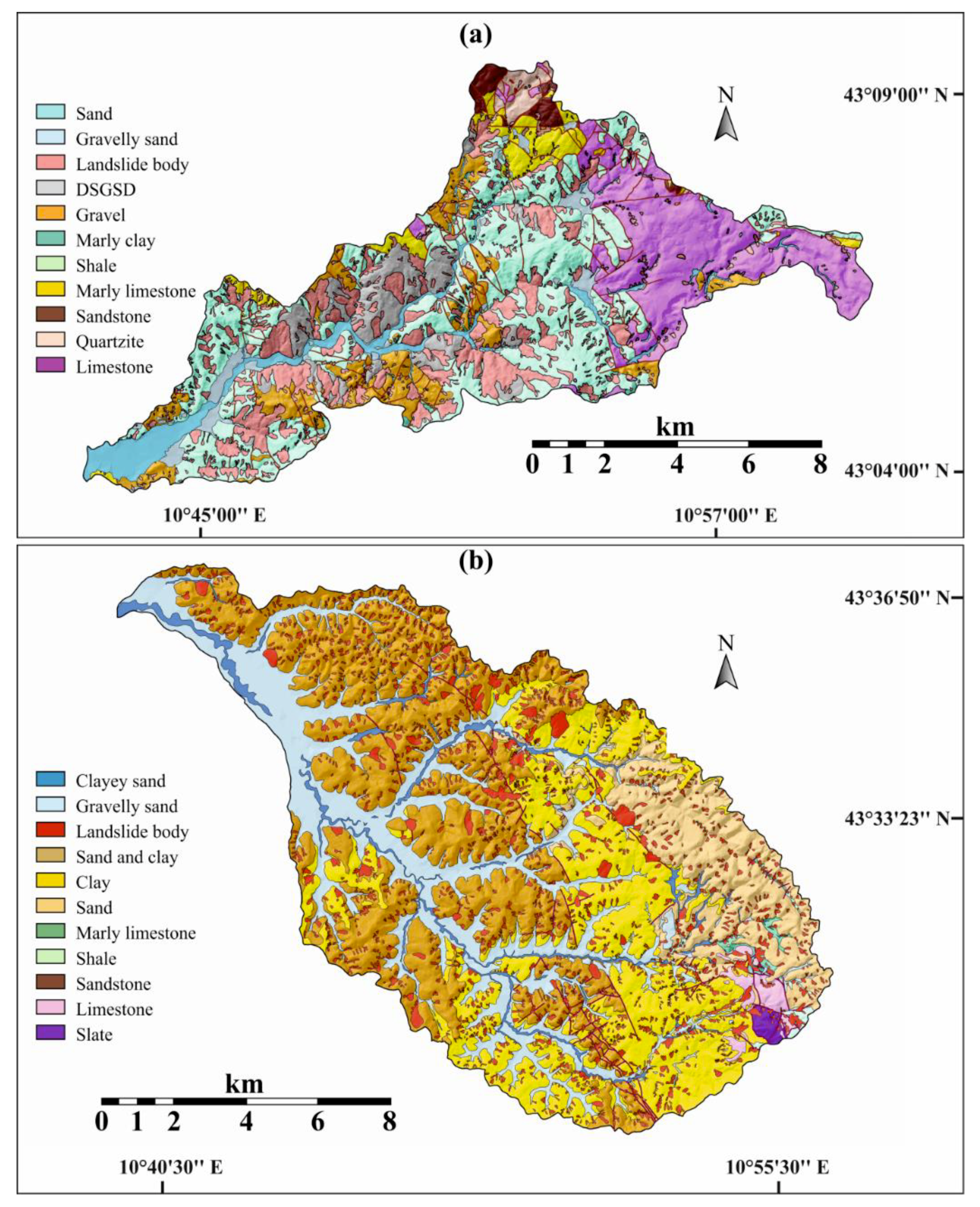
The variables used in this study were selected on the basis of our geomorphological and geological knowledge of the two basins. Lithology, slope angle, slope aspect and distance to hydrographic elements, to tectonic lineaments and to degradation scarps were considered possible landslide-predisposing factors.

The factor maps related to lithology and to the distance from hydrographic elements, from tectonic lineaments and from degradation scarps were attained in vector format from the geological map. For lithology, different classes were extracted from the geological map on the basis of lithological and structural analogies (Figure 4). Considering that many landslides in the study areas occurred from the body of precedent landslides and from DSGSDs [32], it was also necessary to insert these elements into specific classes.

Degradation scarps were indistinctly considered as the edges of the badlands and of the “balze” morphologies. Faults and main thrusts were considered for tectonic lineaments, whereas the main and secondary channels were evaluated for the correlation analysis between landslides and the fluvial activity. The maps related to the distance from hydrographic elements, tectonic lineaments and degradation scarps were performed by subjecting the relative linear feature-class to a process of buffering with the construction of four distance classes based on percentile criteria.

By exploiting the 3D Analyst and Spatial Analyst extensions of ArcInfo, slope angle and slope aspect maps were derived from the 5 × 5 m² pixel resolution DEM, obtained by transforming a TIN (Triangulated Irregular Network) into a GRID. The TIN was generated by the interpolation of digital contour lines and elevation points extracted from the Tuscany Region topographic maps (scale 1:10,000) dating back to 1975. The slope angle was reclassified into six classes with similar areas (percentile criteria), while the slope aspect was reclassified into the eight most frequently adopted classes corresponding to the angular sectors, 45° wide and clockwise from north (equal interval criteria).

Table 1. Area (km²), mean area, area standard deviation (σ), and Main Scarp Upper Edge MSUE density (m²/km²) for each class of the factors used in the analysis. The values are reported for each studied basin.

		Roglio					Milia
Factor	Class	Area (km2)	Mean Area (km2)	σ (km2)	MSUEs Density (103 m2/km2)	Class	Area (km2)	Mean Area (km2)	σ (km2)	MSUEs Density (103 m2/km2)
Lithology (L)	Clayey sand	4.3	0.090	0.197	0	Sand	5.6	0.140	0.701	0
	Gravelly sand	30.3	0.248	1.713	1.0	Gravelly sand	3.1	0.038	0.088	2.6
	Landslide body	16.7	0.004	0.007	8.5	Landslide body	22.4	0.012	0.016	16.7
	Sand and clay	50.6	0.568	1.983	37.7	DSGSD	6.2	0.270	0.468	32.7
	Clay	36.7	0.260	1.194	21.8	Gravel	8.7	0.103	0.143	38.4
	Sand	18.1	0.541	2.643	24.2	Marly clay	0.3	0.018	0.016	52.2
	Marly limestone	0.6	0.021	0.054	23.9	Shale	29.2	0.219	0.922	41.9
	Shale	0.5	0.033	0.040	27.9	Marly limestone	4.0	0.114	0.211	35.3
	Sandstone	0.1	0.005	0.006	28.4	Sandstone	1.5	0.151	0.198	12.0
	Limestone	1.5	0.081	0.142	18.9	Quartzite	1.3	0.262	0.414	7.1
	Slate	0.6	0.312	0.175	26.9	Limestone	19.1	0.515	2.248	5.2
Slope angle (S)	[0–2°]	25.7	0.038	0.122	2.9	[0–4°]	16.5	0.018	0.041	11.1
	[2–7°]	28.2	0.011	0.014	5.4	[4–10°]	16.3	0.034	0.011	16.7
	[7–11°]	26.4	0.063	0.004	10.6	[10–12°]	18.1	0.023	0.005	24.6
	[11–15°]	27.1	0.056	0.003	20.1	[12–15°]	16.6	0.015	0.003	32.3
	[15–21°]	26.2	0.011	0.003	33.4	[15–20°]	17.7	0.018	0.004	31.6
	[21–77°]	26.5	0.057	0.004	55.8	[20–90°]	16.1	0.039	0.040	26.4
Slope aspect (A)	[0–45°]	26.9	0.036	0.017	14.8	[0–45°]	19.6	0.021	0.016	19.0
	[45–90°]	13.8	0.027	0.008	23.7	[45–90°]	6.3	0.018	0.008	37.9
	[90–135°]	13.3	0.039	0.013	28.8	[90–135°]	8.6	0.020	0.002	23.8
	[135–180°]	18.3	0.026	0.012	27.8	[135–180°]	12.9	0.023	0.011	25.0
	[180–225°]	19.1	0.028	0.014	23.5	[180–225°]	13.7	0.021	0.009	25.2
	[225–270°]	22.6	0.018	0.011	18.5	[225–270°]	14.0	0.022	0.011	22.1
	[270–315°]	23.6	0.040	0.013	19.8	[270–315°]	13.6	0.023	0.012	21.8
	[315–0°]	22.7	0.022	0.012	20.1	[315–0°]	12.7	0.024	0.012	27.3
Distance to hydrographic elements (Di)	[0–49 m]	39.5	39.461	0.000	9.1	[0–50 m]	26.6	5.322	9.041	11.1
	[49–105 m]	41.9	0.551	3.409	26.7	[50–110 m]	24.8	0.419	1.242	32.6
	[105–181 m]	40.3	0.183	0.764	25.9	[110–194 m]	25.4	0.153	0.429	25.5
	[181–890 m]	38.6	0.107	0.372	22.9	[194–793 m]	24.5	0.142	0.394	26.3
Distance to tectonic lineaments (Df)	[0–335 m]	39.7	5.763	8.709	23.4	[0–102 m]	24.6	0.491	1.189	29.7
	[335–829 m]	41.5	2.965	8.025	21.1	[102–275 m]	26.3	0.239	0.775	25.4
	[829–1629 m]	40.0	6.671	12.436	20.3	[275–550 m]	24.4	0.669	2.862	23.5
	[1629–7555 m]	38.9	5.563	11.354	20.2	[550–2002 m]	25.1	1.689	2.283	18.1
Distance to degradation scarps (Ds)	[0–60 m]	38.3	0.416	0.803	30.5	N.P.	/	/	/	/
	[60–201 m]	41.9	0.115	0.639	21.3	N.P.	/	/	/	/
	[201–454 m]	40.9	0.584	4.585	17.9	N.P.	/	/	/	/
	[454–1898 m]	39.1	1.563	3.265	15.6	N.P.	/	/	/	/

shows the class extension for each factor and the relative MSUE density.

4.4. Procedure for Selecting the Best LS Model

A Python program (script) in the Model-Builder of ArcInfo was created, in which all the possible combinations of landslide-related factors (UCU maps) were initially computed for each basin. The UCU maps were then intersected with the buffer maps of the MSUEs belonging to the pre-1975 dataset. For each UCU the ratio of the sum of the UCU area that falls within the MSUE buffer and the total area for that UCU can be calculated. The UCUs are thus grouped into five density classes (LS classes) on the basis of the ratio value (UCU density). A similar method, already applied by Clerici et al. [20], is used for class definition. The classes are defined on the basis of MSUE mean density (if, prior probability) obtained by dividing the total MSUE buffer area by the basin area. This value is the middle point of the middle class. More precisely, the class interval on which LS maps are created is Ci = (If/5) × 2 and the susceptibility class intervals are the following: 0–Ci (Very Low), Ci–2Ci (Low), 2Ci–3Ci (Medium), 3Ci–4Ci (High) and 4Ci–5Ci (Very High).

The validation procedure was performed in the Model-Builder to choose the best model. Considering that the validation procedure is based on the “wait and see” concept, the distribution of the pre-1975 MSUEs (training set) is compared to that of the post-1975 MSUEs (validation set). More specifically, the absolute value of the difference between the pre-1975 and post-1975 MSUE percentage is computed for each LS class. The sum of the latter values, Validation Error (VE), is reported for each LS model. The VE assesses the predictive power of each model built and its value ranging from 0 (the best predictive power) to 200 (worst predictive power).

According to Clerici et al. [20], a good model should have a great dispersion around the landslide mean density value to distinguish among significantly different landslide density conditions. Therefore, we computed the mean deviation (MD) of the UCU density for each model and we used the ratio MD/(0.01 + VE) (Best Model Index, BMI) to choose the best LS model, which should have the highest BMI value.

The procedure proposed by Clerici et al. [20] to select the best model is very similar to that proposed by Chung and Fabbri [23], frequently used in recent researches [8,11,36,37]. Considering that UCU ordering within a Success Rate Curve (SRC) should be made according to landslide density (conditional probability), the higher the UCU-density mean deviation (MD), the greater the area under the curve (AUC) of the SRC. Furthermore, the lower the VE model, the smaller the AUC difference between the Prediction Rate Curve (PRC) and the SRC of the model. As a whole, the higher the value of the BMI, the better the fitting performance and prediction skill of the LS model.

However, in areas such as the Roglio and Milia basins, where a large portion of the basin surface is covered by landslides, it is impossible to obtain steep Success Rate Curves [38].

The conditional analysis method applied to factor combinations does not require the inter-correlation analysis between predisposing factors. If some of the factors introduced in the analysis are strictly related to each other, providing redundant information, the models attained from the combination will have a lower BMI than that of the models built from spatial independent predisposing factors.

Since BMI unifies the two types of errors (false positives and false negatives), and false negatives are more dangerous for susceptibility analysis, the validation system proposed by Clerici et al. [20] was here also supported by the analysis of the model receiver operating the characteristic (ROC) curve [12,23,39,40,41].

4.5. Statistical Significance of the Best Model

Independently of the procedure chosen for the best LS model selection, all the methods used to select the LS model performance gave us the best LS model among those built without any clues regarding the possibility of obtaining a better model for the same input landslide datasets (training and validation). More specifically, the procedure chosen for the best LS model selection did not provide us with any information about the possibility of obtaining a better LS model by changing the terrain map unit, factor map quality, and the procedure used for factor-classes subdivision, landslide-predisposing factors, and statistical analysis method. In other words, we cannot define how statistically significant is the assertion according to which the best possible LS model is the one chosen from our study.

An analysis of the reduced chi-square (Ӽ²) was performed to define how the predictive ability of the best model actually represents the Ӽ² maximum likelihood among the landslide groups used for model construction and validation. Independently of the system (statistical methods, landslide-relating factor, model validation procedures and map units) used to divide the territory and to reclassify it into five susceptibility classes, the reduced chi-square allowed us to obtain models with a higher likelihood degree than those obtained in the study. The Ӽ² value for a model defines the probability of finding a likelihood between the observed and the expected probability of a certain event A, which is better than that defined by the model itself [42,43,44]. Considering that the forecasting model should be made by using an older landslide inventory, and that more recent landslides should be used to evaluate the prediction [21,22,23,38], for each model the percentage of landslides belonging to the validation group that fall into a susceptibility class must be necessarily considered as the expected values of the landsliding probability in that class.

Therefore, in this study the chi-square value is calculated as follows:

$${\mathrm{Ӽ}}^2=\frac{1}{\mathrm{n}-1}{{\displaystyle \sum }}_{\mathrm{i}=1}^{\mathrm{n}}\frac{{\left[\left(\%\mathrm{MSUE}\mathrm{buffer}\mathrm{area}\mathrm{pre}-75\right)\mathrm{i}-\left(\%\mathrm{MSUE}\mathrm{buffer}\mathrm{area}\mathrm{post}-75\right)\mathrm{i}\right]}^2}{\left(\%\mathrm{MSUE}\mathrm{buffer}\mathrm{area}\mathrm{post}-75\right)\mathrm{i}}$$

where n is the LS model class number.

5. Results and Discussion

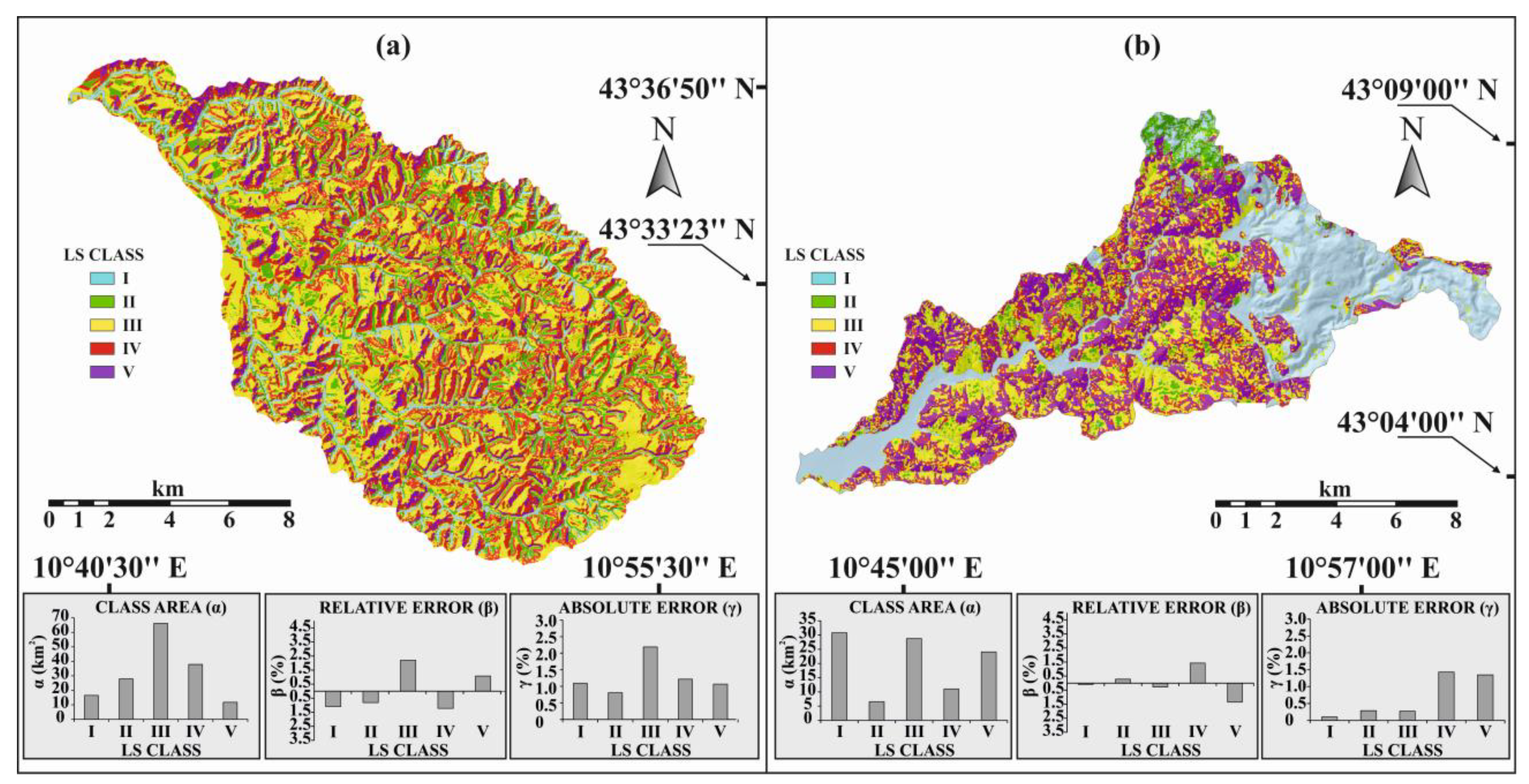
A total of 63 and 31 translational slide susceptibility models were made for the Roglio and Milia basins.

Table 2. The 10 best models of landslide susceptibility obtained for each basin. FC: Factors combination (L: Lithology, S: Slope angle, A: Slope aspect, Di: Distance to hydrographic elements, Df: Distance to tectonic lineaments, Ds: Distance to degradation scarps); VE: Validation error (%); MD: Mean deviation (m²/km²); BMI: Best model index (km²/m²); ROC AUC (%); Area Under the ROC Curve; ROC: receiver operating characteristic curve.

		ROGLIO BASIN					MILIA BASIN
FC	VE	MD	BMI	ROC AUC	FC	VE	MD	BMI	ROC AUC
	(%)	(103 m2/km2)	(102 km2/m2)	(%)		(%)	(103 m2/km2)	(102 km2/m2)	(%)
ADiDf	6.3	3.63	5.75	87.9	LS	3.4	8.57	25.13	87.3
LDiDf	25.2	8.45	3.35	82.1	LDi	9.1	8.78	9.64	85.2
ADi	5.5	2.34	4.25	81.5	LSDf	11.0	8.89	8.07	84.5
LDi	20.5	8.96	4.37	80.1	LDiDf	5.6	9.04	16.11	82.0
LADi	25.5	11.24	4.41	79.1	LA	11.8	8.78	7.43	80.8
LSADi	29.2	14.14	4.84	78.5	LDf	5.5	8.08	14.66	79.9
LADiDf	27.9	10.59	3.79	77.2	LSA	11.7	10.49	8.96	79.6
LSDiDf	25.2	10.31	4.01	75.0	LADi	13.2	10.66	8.07	77.7
ADfDs	12.1	3.52	2.91	71.6	LSDiDf	16.4	11.03	6.72	77.5
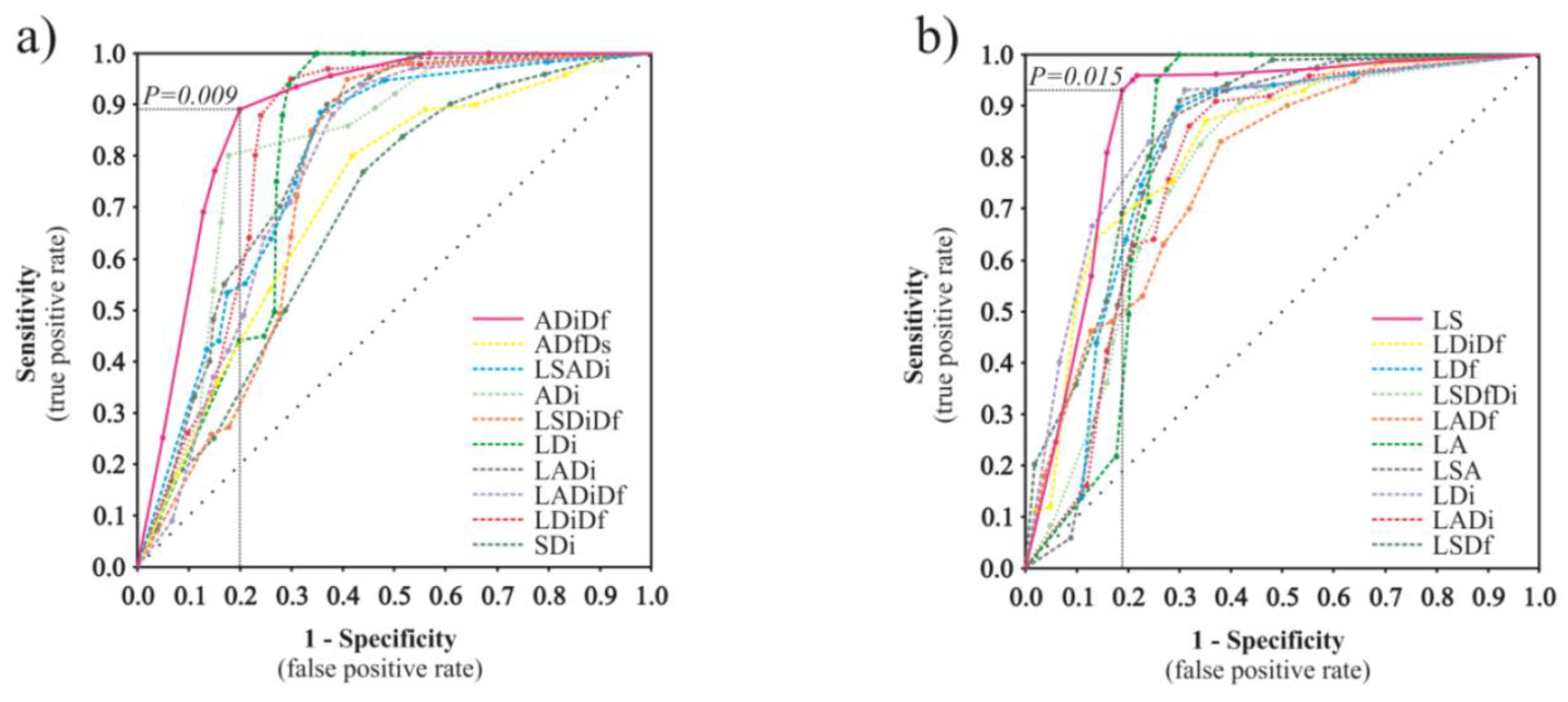
SDi	24.5	8.20	3.34	68.8	LADf	16.0	9.52	5.95	77.3

shows the 10 models with the highest area under the ROC curve (AUC) for both basins. The best model of each basin is related to the environmental factor combination (FC) characterizing the first row of the table, which also shows the highest BMI. In the Milia basin, the combination of the lithology-slope angle (LS) factors represents the best model with an AUC = 87.3 and a BMI = 2513.1 (Table 2). In the Roglio basin, the combination of aspect–distance to hydrographic elements and distance to tectonic lineaments (ADiDf) factors represents the best model with an AUC = 87.9 and a BMI = 575.0 (

Table 3. Chi-square statistics of the best models. The chi-square tests were performed with 4 degree of freedom and 0.05 confidence level (Ӽ²_critic = 0.177) and with 9 degree of freedom and 0.05 confidence level (Ӽ²_critic = 0.369).

		Four Degree of Freedom		Nine Degree of Freedom
Roglio-LS best model	VE	Ӽ2obs.	P (Ӽ2< Ӽ2obs.)	Ӽ2obs.	P (Ӽ2< Ӽ2obs.)
ADiDf	6.3	0.175	< 0.05	0.263	< 0.05
Milia-LS best model	VE	Ӽ2obs.	P (Ӽ2< Ӽ2obs.)	Ӽ2obs.	P (Ӽ2< Ӽ2obs.)
LS	3.4	0.049	< 0.05	0.261	< 0.05

)

The two best models provide satisfactory results (Figure 5). For the first model of the Roglio basin, at the cutoff probability level of 0.009, 84.8% of the UCUs are correctly classified (model efficiency), whereas in the Milia basin, at the cutoff probability level of 0.015, the efficiency of the best model reaches 84.5%. Both cutoff values correspond to the limits between high and very high susceptibility classes of the best two models.

For the translational slides of the Roglio basin, the best model has a reduced ability to discriminate the susceptibility of the UCUs compared to the prior probability, although it is characterized by a low validation error. In this case the MD value equal to 3629 implies a concentration of UCUs in the medium susceptibility class (Figure 6a).

The Ӽ² determination allows us to carry out the consideration about which model approaches the maximum likelihood with an acceptable statistical significance (p [Ӽ² < Ӽ²observed] ≤ 0.05). In addition, as all the chosen models have been created with the same number of degrees of freedom (number of classes of susceptibility −1), the analysis of Ӽ² allows us to compare the predictive capabilities of each of these models. Regardless of how the territory was divided and reclassified into five classes of susceptibility (statistical methods, model validation procedures, and map units used), the likelihood degree of the models is always calculated on the same Ӽ² probability distribution curve (integral function of Pugh and Winslow [42]), which is related to systems with four degrees of freedom (Ӽ²_critic = 0.177 for 0.05 confidence level).

The values obtained were compared to the probability table of Ӽ² with four degrees of freedom [42,44], and the probabilities P(Ӽ² < Ӽ²observed.) have been determined for each best model (Table 3).

From the reduced Ӽ² analysis, it is possible to see how the best models in the Roglio and Milia basins show an acceptable predictive power, where the combination of the factors, slope aspect, distance to the hydrographic elements and distance to tectonic lineaments (ADiDf) for the first, lithology and slope angle (LS) for the second are the best models with a good statistical significance level. In other words, the assertion for which in the Milia and Roglio basins the best LS models are the best possible can be accepted at the 95 percent level.

The good statistical significance level of the two best models does not change by increasing the degrees of freedom of the chi-square test (Table 3). Moving from four to nine degree of freedom, i.e., the maximum value for which we can avoid models class frequency lower than 5%, the probability of obtaining models with a higher likelihood degree than those carried out from this study are yet less than 0.05 (Ӽ²_critic = 0.369 for 0.05 confidence level).

Therefore, for the Milia and Roglio basins we have convincing evidences that MSUE is efficient at yielding relevant LS maps for predicting the translational slide-type landslide.

6. Conclusions

In this study, we analyzed the applicability of the MSUE, as dependent variable representation, in the LS zonation of two Tuscany basins. The results show how for translational slides the use of the MSUE yields models with a very high power prediction. Regardless of the mode (statistical methods, factor map quality, models validation procedures and map units) used to divide the territory and to reclassify it into five susceptibility classes, the probability of obtaining models with a higher likelihood degree than those carried out for the translational slides of the studied basins is lower than 0.05. In particular, the model created for the translational slides of the Milia basin appears surprisingly exceptional in predicting landslide development with a high spatial resolution. In the Roglio basin, slope angle, distance from streams and from tectonic lineaments have demonstrated to be the main controlling factors of translational slides. The high translational slide susceptibility zones are primarily located in the SE-facing slopes adjacent to streams and to tectonic lineaments. In the Milia basin, lithology and slope angle gave more satisfactory results as landslide-predisposing factors. More specifically, the susceptibility map of the translational slides outlines hillslope sections where shale formations outcrop, with a slope gradient above 33%, as very prone to landslides.

Overall, for translational slide-type landslides, the study results show how MSUE can be applied as dependent variable representation to landslide susceptibility zonation with appreciable results.

MSUE applicability to other landslide typologies, however, still remains unresolved and it should be studied in future works together with the MSUE applicability on lithotypes and geomorphological conditions different from those considered in this study.

References

- Bathrellos, G.D.; Gaki-Papanastassiou, K.; Skilodimou, H.D.; Papanastassiou, D.; Chousianitis, G. Potential suitability for urban planning and industry development using natural hazard maps an geological-geomorphological parameters. Environ. Earth Sci. 2012, 66, 537–548. [Google Scholar] [CrossRef]
- Bathrellos, G.D.; Skilodimou, H.D.; Chousianitis, K.; Youssef, A.M.; Pradhan, B. Suitability estimation for urban development using multi-hazard assessment map. Sci. Total Environ. 2017, 575, 119–134. [Google Scholar] [CrossRef] [PubMed]
- Brabb, E. Innovative approaches to landslide hazard mapping. In Proceedings of the IV International Symposium Landslides, Toronto, ON, Canada, 16–21 September 1984; pp. 307–324. [Google Scholar]
- Soeters, R.; van Westen, C.J. Slope instability recognition, analysis, and zonation. In Landslides Investigation and Mitigation; Turner, A.K., Schuster, R.L., Eds.; Special Report 247; Transportation Research Board, National Research Council: Washington, DC, USA, 1996; pp. 129–177. [Google Scholar]
- Guzzetti, F.; Carrara, A.; Cardinali, M.; Reichenbach, P. Landslide hazard evaluation: A review of current techniques and their application in a multi-scale study, Central Italy. Geomorphology 1999, 31, 181–216. [Google Scholar] [CrossRef]
- Regmi, N.R.; Giardino, J.R.; Vitek, J.D. Modeling susceptibility to landslides using the weight of evidence approach: Western Colorado, USA. Geomorphology 2010, 115, 172–187. [Google Scholar] [CrossRef]
- Regmi, N.R.; Giardino, J.R.; Vitek, J.D.; Dangol, V. Mapping landslide hazards in western Nepal: Comparing qualitative and quantitative approaches. Envrion. Eng. Geosci. 2010, 16, 127–142. [Google Scholar] [CrossRef]
- Sterlacchini, S.; Ballabio, C.; Blahut, J.; Beretta, G.; Facchi, A. Spatial agreement of predicted patterns in landslide susceptibility maps. Geomorphology 2011, 125, 51–61. [Google Scholar] [CrossRef]
- Cardinali, M.; Carrara, A.; Guzzetti, F.; Reichenbach, P. Landslide Hazard Map for the Upper Tiber River Basin; Gruppo Nazionale per la Difesa dalle Catastrofi Idrogeologiche Publication: Perugia, Italy, 2002. [Google Scholar]
- Clerici, A.; Perego, S.; Tellini, C.; Vescovi, P. A GIS-based automated procedure for landslide susceptibility mapping by the conditional analysis method: The Baganza valley case study (Italian Northern Apennines). Envrion. Geol. 2006, 50, 941–961. [Google Scholar] [CrossRef]
- Conforti, M.; Robustelli, G.; Muto, F.; Critelli, S. Application and validation of bivariate GIS-based landslide susceptibility assessment for the Vitravo river catchment (Calabria, south Italy). Nat. Hazards 2012, 61, 127–141. [Google Scholar] [CrossRef]
- Conoscenti, C.; Rotigliano, E.; Cama, M.; Caraballo-Arias, N.A.; Lombardo, L.; Agnesi, V. Exploring the effect of absences selection on landslide susceptibility models: A case study of Sicily, Italy. Geomorphology 2016, 261, 222–235. [Google Scholar] [CrossRef]
- Hong, H.; Ilia, I.; Tsangaratos, P.; Chen, W.; Xu, C. A hybrid fuzzy weight of evidence method in landslide susceptibility analysis on the Wuyuan area, China. Geomorphology 2017, 290, 1–16. [Google Scholar] [CrossRef]
- Carrara, A.; Cardinali, M.; Guzzetti, F.; Reichenbach, P. GIS technology in mapping landslide hazard. In Geographical Information Systems in Assessing Natural Hazards; Carrara, A., Guzzetti, F., Eds.; Kluwer Academic Publisher: Dordrecht, The Netherlands, 1995; pp. 135–175. [Google Scholar]
- Süzen, M.L.; Doyuran, V. Data-driven bivariate landslide susceptibility assessment using geographical information systems: A method and application to Asarsuyu catchment, Turkey. Eng. Geol. 2004, 71, 303–321. [Google Scholar] [CrossRef]
- Havenith, H.B.; Strom, A.; Caceres, F.; Pirard, E. Analysis of landslide susceptibility in the Suusamyr region, Tien Shan: Statistical and geotechnical approach. Landslides 2006, 3, 39–50. [Google Scholar] [CrossRef]
- Havenith, H.B.; Torgoev, I.; Meleshko, A.; Alioshin, Y.; Torgoev, A.; Danneels, G. Landslides in the Mailuu-Suu Valley, Kyrgyzstan—Hazards and impacts. Landslides 2006, 3, 137–147. [Google Scholar] [CrossRef]
- Nefeslioglu, H.A.; Duman, T.Y.; Durmaz, S. Landslide susceptibility mapping for a part of tectonic Kelkit Valley (Eastern Black Sea region of Turkey). Geomorphology 2008, 94, 401–418. [Google Scholar] [CrossRef]
- Vergari, F.; Della Seta, M.; Del Monte, M.; Fredi, P.; Palmieri, E. Landslide susceptibility assessment in the Upper Orcia Valley (Southern Tuscany, Italy) through conditional analysis: A contribution to the unbiased selection of causal factors. Nat. Hazards Earth Syst. 2011, 11, 1475–1497. [Google Scholar] [CrossRef]
- Clerici, A.; Perego, S.; Tellini, C.; Vescovi, P. Landslide failure and runout susceptibility in the upper T. Ceno valley (Northern Apennines, Italy). Nat. Hazards 2010, 52, 1–29. [Google Scholar] [CrossRef]
- Guzzetti, F.; Reichenbach, P.; Ardizzone, F.; Cardinali, M.; Galli, M. Estimating the quality of landslide susceptibility models. Geomorphology 2006, 81, 166–184. [Google Scholar] [CrossRef]
- Chung, C.F.; Fabbri, A.G. Predicting landslides for risk analysis—Spatial models tested by a cross-validation procedure. Geomorphology 2008, 94, 438–452. [Google Scholar] [CrossRef]
- Von Ruette, J.; Papritz, A.; Lehmann, P.; Rickli, C.; Or, D. Spatial statistical modeling of shallow landslides—Validating predictions for different landslide inventories and rainfall events. Geomorphology 2011, 133, 11–22. [Google Scholar] [CrossRef]
- Clerici, A.; Perego, S.; Tellini, C.; Vescovi, P. A procedure for landslide susceptibility zonation by the conditional analysis method. Geomorphology 2002, 48, 349–364. [Google Scholar] [CrossRef]
- Chung, C.F.; Fabbri, A.G. Probabilistic prediction models for landslide hazard mapping. Photogramm. Eng. Remote Sens. 1999, 65, 1389–1399. [Google Scholar]
- Costantini, A.; Lazzarotto, A.; Liotta, D.; Mazzanti, R.; Mazzei, R.; Salvatorini, G.F. Note Illustrative Della Carta Geologica d’Italia alla Scala 1:50.000, Foglio 306—Massa Marittima; Servizio Geologico d’Italia: Roman, Italy, 2000; p. 174. [Google Scholar]
- Costantini, A.; Lazzarotto, A.; Mazzanti, R.; Mazzei, R.; Salvatorini, G.F.; Sandrelli, F. Note Illustrative Della Carta Geologica d’Italia alla Scala 1:50.000, Foglio 285—Volterra; Servizio Geologico d’Italia: Roman, Italy, 2002; p. 154. [Google Scholar]
- Carmignani, L.; Decandia, F.A.; Fantozzi, P.; Lazzarotto, A.; Liotta, D.; Meccheri, M. Tertiary extensional tectonics in Tuscany (Northern Apennines, Italy). Tectonophysics 1994, 238, 295–315. [Google Scholar] [CrossRef]
- Cruden, D.M.; Varnes, D.J. Landslide types and processes. In Landslides Investigation and Mitigation; Turner, A.K., Schuster, R.L., Eds.; Special Report 247; Transportation Research Board, National Research Council: Washington, DC, USA, 1996; pp. 36–75. [Google Scholar]
- Dramis, F.; Sorriso-Valvo, M. Deep seated slope deformations, related landslide and tectonics. Eng. Geol. 1994, 38, 231–243. [Google Scholar] [CrossRef]
- Zischinsky, U. Uber Sackungen. Rock Mech. 1969, 1, 30–52. [Google Scholar] [CrossRef]
- Capitani, M.; Ribolini, A.; Federici, P.R. Influence of deep-seated gravitational slope deformations on landslide distributions: A statistical approach. Geomorphology 2013, 201, 127–134. [Google Scholar] [CrossRef]
- Mazzanti, R. Geologia della zona di Montaione tra le valli dell’Era e dell’Elsa (Toscana). Boll. Soc. Geol. Ital. 1961, 73, 37–126. [Google Scholar]
- Morgan, B.W. An Introduction to Bayesian Statistical Decision Process; Prentice-Hall: New York, NY, USA, 1968. [Google Scholar]
- Keefer, D.K. Landslides caused by earthquakes. Geol. Soc. Am. Bull. 1984, 95, 406–421. [Google Scholar] [CrossRef]
- Piacentini, D.; Troiani, F.; Soldati, M.; Notarnicola, C.; Savelli, D.; Schneiderbauer, S. Statistical analysis for assessing shallow-landslide susceptibility in South Tyrol (south-eastern Alps, Italy). Geomorphology 2012, 151, 196–206. [Google Scholar] [CrossRef]
- Poiraud, A. Landslide susceptibility–certainty mapping by a multi-method approach: A case study in the Tertiary basin of Puy-en-Velay (Massif central, France). Geomorphology 2014, 216, 208–224. [Google Scholar] [CrossRef]
- Blahut, J.; van Westen, C.J.; Sterlacchini, S. Analysis of landslide inventories for accurate prediction of debris-flow source areas. Geomorphology 2010, 119, 36–51. [Google Scholar] [CrossRef]
- Fawcett, T. An introduction to ROC analysis. Pattern Recognit. Lett. 2006, 27, 861–874. [Google Scholar] [CrossRef]
- Van Den Eeckhaut, M.; Vanwalleghem, T.; Poesen, J.; Govers, G.; Verstraeten, G.; Vanderkerckhove, L. Prediction of landslide susceptibility using rare events logistic regression: A case-study in the Flemish Ardennes (Belgium). Geomorphology 2006, 76, 392–410. [Google Scholar] [CrossRef]
- Rossi, M.; Guzzetti, F.; Reichenbach, P.; Mondini, A.; Perucacci, S. Optimal landslide susceptibility zonation based on multiple forecasts. Geomorphology 2010, 114, 129–142. [Google Scholar] [CrossRef]
- Pugh, E.M.; Winslow, G.H. The Analysis of Physical Measurements; Addison-Wesley: London, UK, 1966. [Google Scholar]
- Kendall, M.; Stuart, A. The Advanced Theory of Statistics: Inference and Relationship; Griffin: London, UK, 1979. [Google Scholar]
- Buccianti, A.; Rosso, F.; Vlacci, F. Metodi Matematici e Statistici nelle Scienze della Terra. Tecniche Statistiche; Liguori: Napoli, Italy, 2003. [Google Scholar]
© 2018 by the authors. Licensee MDPI, Basel, Switzerland. This article is an open access article distributed under the terms and conditions of the Creative Commons Attribution (CC BY) license (http://creativecommons.org/licenses/by/4.0/).