Article

A Segmented Processing Approach of Eigenvector Spatial Filtering Regression for Normalized Difference Vegetation Index in Central China

1
School of Resource and Environment Science, Wuhan University, Wuhan 430079, China
2
Wuda Geoinformatics Co., Ltd., Wuhan 430000, China
*
Author to whom correspondence should be addressed.
ISPRS Int. J. Geo-Inf. 2018, 7(8), 330; https://doi.org/10.3390/ijgi7080330
Submission received: 5 July 2018 / Revised: 27 July 2018 / Accepted: 7 August 2018 / Published: 17 August 2018

Abstract

:
A segmented processing approach of eigenvector spatial filtering (ESF) regression is proposed to detect the relationship between NDVI and its environmental factors like DEM, precipitation, relative humidity, precipitation days, soil organic carbon, and soil base saturation in central China. An optimum size of 32 × 32 is selected through experiments as the basic unit for image segmentation to resolve the large datasets to smaller ones that can be performed in parallel and processed more efficiently. The eigenvectors from the spatial weights matrix (SWM) of each segmented image block are selected as synthetic proxy variables accounting for the spatial effects and aggregated to construct a global ESF regression model. Results show precipitation and humidity are more influential than other factors and spatial autocorrelation plays a vital role in vegetation cover in central China. Despite the increase in model complexity; the parallel ESF regression model performs best across all performance criteria compared to the ordinary least squared linear regression (OLS) and spatial autoregressive (SAR) models. The proposed parallel ESF approach overcomes the computational barrier for large data sets and is very promising in applying spatial regression modeling to a wide range of real world problem solving and forecasting.

1. Introduction

Vegetation cover is one of the most important indicators for ecological environment. Thus, it is important to study vegetation cover indicators and their relations with the influenced factors. Normalized Difference Vegetation Index (NDVI) has been proved to be an effective indicator for green vegetation cover on the earth surface, which is defined as NDVI = (NIR − Red)/(NIR + Red), in which NIR is the reflectance of the near-infrared wavelength band and Red is the reflectance of the red wavelength band [1]. The relationship has been established well between NDVI and vegetation cover [2]. Environmental factors for green vegetation growth and the relationship between NDVI and other factors have been detected. Possible factors come as precipitation, elevation, moisture, soil compositions, and so on [3,4,5,6]. The correlation between NDVI, temperature, and precipitation varies considerably in different places and in different seasons [3,7,8,9,10]. However, conventional analysis methods are often based on regression analysis with observation data from meteorological stations or sampling schemes like random, regular, and stratified, which take a subset out to represent the population from remote sensing imagery data. Absence of spatial information in regression models may cause variance inflation and increase model uncertainty [11,12]. For example, an algorithm was reported to predict NDVI using precipitation data and air temperature data on the earth surface with a spatial resolution of 0.25° × 0.25° on the globe [13]. However, it has limited values for inference and prediction, as the model does not account for spatial autocorrelation; it works only in arid and semi-arid regions, and the resolution is too coarse for a broad application [13].
In recent years, spatial statistics models considering spatial autocorrelation are being used by econometrics scientists. From the dynamic classification pattern based on formal concept analysis for spatial statistics services, the Spatial Autoregressive (SAR) model and Spatial Filtering model can be used to deal with regression matters containing spatial autocorrelation [14]. However, the usefulness of the SAR model is limited for large datasets, because the maximum likelihood estimation for parameters may be computationally prohibitive for large datasets [15]. Eigenvector Spatial Filtering provides a flexible approach with which to solve the problem of spatial autocorrelation in regression by separating spatial effects from the variables’ total effects [16]. In spatial data analysis, enhanced and robust results can be obtained by spatial filtering [17]. Not only trends and spatially structured random components can be decomposed from the variable, but spatial noise can be filtered out. Griffith proposed eigenvector spatial filtering (ESF) methodology to filter out spatial autocorrelation from the variables’ total effects. Filtering is based on a decomposition of the spatial weights matrix used for computing the Moran Coefficient (MC) [18]. Spatial autocorrelation can be accounted for successfully by the ESF method, which can be incorporated to not only OLS but also Generalized Linear Models and Generalized Linear Mixed Models [19,20]. The usefulness of separating spatial effects from variables’ total effects by ESF approach has been demonstrated in ecological and socio-economic fields [21,22,23] in which ESF regression analysis usually takes administrative units as the study unit or sampling points to represent the study region. In other words, these applications are vector-based and today’s computers can handle the amount of computation. Modeling with NDVI, however, is best done in the raster data model, which in turn is facing the computational problem as the spatial weights matrix is prohibitively large, because for an n-by-n image, the SWM is n 2 × n 2 . Even though one can use analytical methods to approximate the eigenfunction for regular lattices [24], the selection of eigenvectors would take too long to complete within a reasonable duration. A temporal filtering algorithm was reported to minimize the contamination by cloud and noise in the NDVI time series, but it does not deal with spatial effects in regression modeling and is suitable in Australia [25]. Although a Fourier Filter was applied to minimize the influence of high-frequency noise in NDVI classification, it does not take environmental factors into consideration [26].
We explored a parallel ESF method to address the computational problem. The parallel ESF method resolves the large datasets to smaller ones and utilizes the multicore CPU of personal computers as workers to construct a cluster to execute the ESF regression process simultaneously [27]. An optimum segmented size of 32 × 32 is selected through experiments as the basic unit for image segmentation. The large datasets are segmented to a group of datasets of the same size 32 × 32 and launched together with a new copy of ESF regression code to each worker in the cluster. After the compute tasks for each segments are completed, the client will collect the results from all worker sessions [28]. In this way, the resolved smaller datasets can be calculated easily, and the compute process is accelerated efficiently.
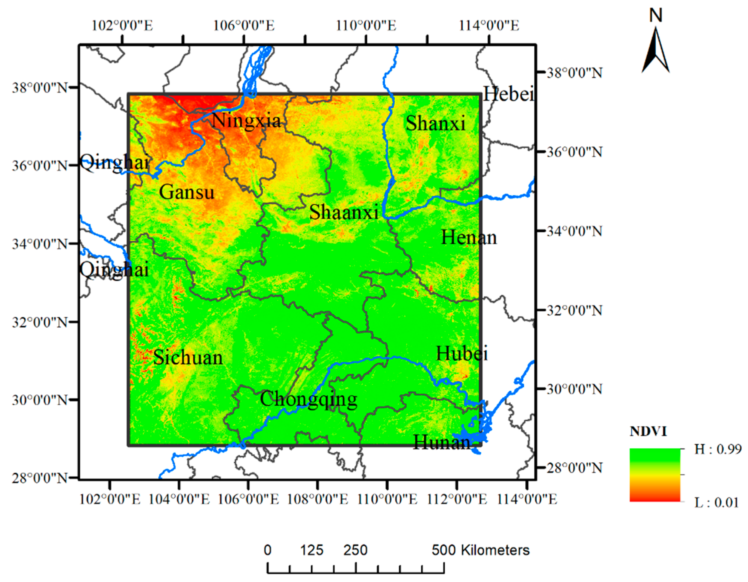
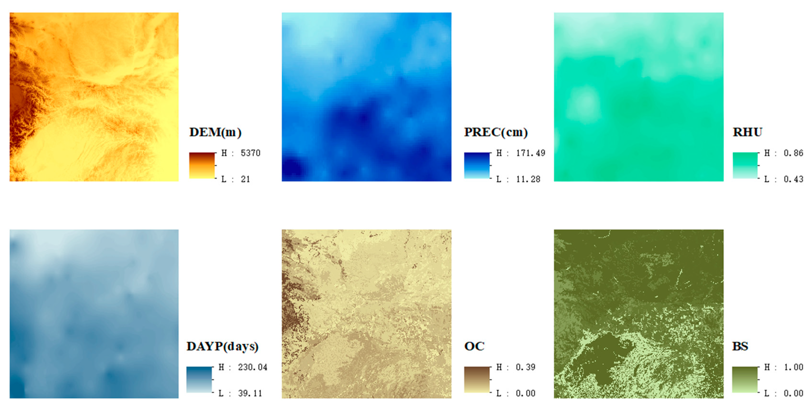
In this study, raster datasets of NDVI and environmental factors including DEM, precipitation (PREC), relative humidity (RHU), precipitation days greater than 0.1 mm (DAYP), soil organic carbon (OC), and soil base saturation (BS) content in central China are employed and segmented to squared blocks to construct the Parallel-ESF regression model. This method is expected to improve the goodness of fit of the regression model by taking the spatial autocorrelation of variables into consideration and accelerating the computation process for large raster datasets. The aim is to study the correlation of environmental factors for NDVI in central China, which will consider the spatial effects that existed in variables. Moreover, this paper attempts to provide the feasible access of the segmented processing approach to solve the problem of spatial autocorrelation and the memory insufficiency of eigenvectors generation using the ESF regression approach for large size raster datasets.

2. Methodology

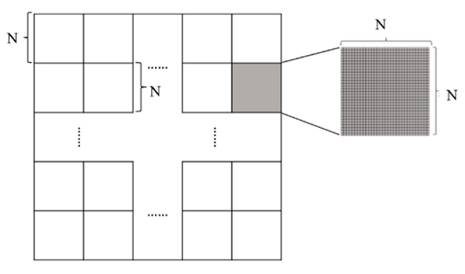
The proposed methodology contains 4 steps in this study. The first step is to estimate the optimum size of the N × N image blocks and segment the large datasets in a mutually exclusive and collectively exhaustive manner. The second step is to construct the spatial weights matrix based on contiguity relation for N × N squared blocks and its eigenfunction. The third step is to estimate regression model with selected eigenvectors included for each segmented blocks. The last step is to compare the model performance of the local ESF regression models with the conventional multiple linear regression model and the spatial autoregressive model.

2.1. Raster Segmentation

As indicated earlier, calculation of the eigenfunction and selection of eigenvector through step-wise regression can be very time consuming, especially for raster data. Tests of linear ESF are conducted on various size such as 8 × 8, 16 × 16, 32 × 32, 64 × 64, and so on, as Figure 1 shows. The optimum subset size takes both time costs of eigenvectors selection for a single block and the number of all segmented blocks into consideration. Smaller size of subsets is more efficient for calculation, but more subsets mean more information loss from more separated pixels. Time costs of eigenvector selection in various size images are obtained to choose acceptable elapsed time for a single image block. The result shows that the computer is stress-free for the raster of the sizes 8 × 8, 16 × 16, and 32 × 32 to generate eigenvectors from spatial weights matrix, and it takes a few minutes for size 64 × 64 to generate eigenvectors. However, in the process of identifying eigenvectors, especially the permutation test in stepwise regression, the computer exports no result, causing computers to halt for the size 64 × 64. Considering the number of segmented blocks and loss of efficiency in task and data transmitting procedure, size 32 × 32 is selected as the basic unit for image segmentation. Once the optimum subset size is determined, the image datasets representing the dependent variable and the predictor variables are segmented to a group of squared blocks. Note that preprocess of resize should be conducted to ensure all datasets have the same resolution.

2.2. Eigenvector Generation Based on SWM

Topology-based spatial weights matrix for the image block serves as the base for representing spatial relationship in regression models [18]. For square tessellations, queen contiguity is adopted to construct the binary spatial weights matrix C with c i j = 1 if the two cells are neighbors and c i j = 0 otherwise [29]. The spatial weights matrices are the same for all segmented blocks and can be calculated only once, because the image blocks have identical spatial weights matrices. The spatial weights matrix is subsequently centered through the projection matrix as follows:
( I 11 T / n ) C ( I 11 T / n )
in which 1 is an n × 1 vectors of ones. The symbol T donated the matrix transpose operator.
The eigenfunction, containing eigenvectors and associated eigenvalues, is calculated from decomposition of the modified spatial weights matrix [30]. The decomposition can be expressed as
MCM = E Λ E T
in which M = ( I 11 T / n ) . The character Λ is an n × n diagonal matrix of eigenvalues ( λ 1 , λ 2 , , λ n ) in descending order. E = ( E 1 , E 2 , , E n ) are the eigenvectors corresponding to the eigenvalues Λ [22]. For being orthogonal and uncorrelated, each eigenvector can portray distinct map patterns with achievable level of spatial autocorrelation for a given geographic landscape [31]. The function relation has been detected between MC value for a mapped eigenvector and its corresponding eigenvalue as follows:
MC j = n 1 T C 1 λ j
Based upon these properties, the eigenvectors can be interpreted as follows: The first eigenvector E 1 is the set of real numbers that has the largest MC achievable by any set for the geographic arrangement defined by the spatial connectivity matrix C . The second eigenvector E 2 is the set of real numbers that has the largest achievable MC by any set that is orthogonal and uncorrelated with E 1 . So on through the nth eigenvector E n , which is the set of real numbers that has the largest negative MC achievable by any set that is orthogonal and uncorrelated with the preceding ( n 1 ) eigenvectors [32]. Being mutually orthogonal and uncorrelated, these eigenvectors can cause the emergence of latent spatial autocorrelation in variables [21], and those eigenvectors that are significant can be filtered out and act as proxies in explanatory variable to capture its spatial stochastic component [19].

2.3. Parallel Eigenvector Filtering

Since the eigenvectors of spatial weights matrix portray a different map pattern exhibiting a specified level of spatial autocorrelation, a parallel processing approach is adopted to select the significant eigenvectors E k in each block as control variables in a linear combination and construct a global ESF regression model for all the segmented blocks. The identification of E k can be achieved by a forward stepwise selection procedure. The criteria to identify eigenvectors contain significance level of the estimated coefficients and Akaike Information Criteria (AIC) of model at each step.
Before the stepwise selection, a candidate set of eigenvectors, a smaller subset of the entire eigenvectors, can be demarcated by the properties of eigenvectors to reduce workload. Eigenvectors whose MC values can be eliminated, because these eigenvectors do not explain much spatial variation. Second, eigenvectors that represent negative SA can be excluded, because empirical NDVI displays positive SA. A feasible criterion for eigenvectors identification is λ divided by the largest eigenvalue λ m a x that is greater than 0.25 [33].
The parallel processing approach takes segmented dataset in each block and the candidate set of eigenvectors together to run the stepwise process. For each block, eigenvectors are selected via conventional stepwise regression procedures from the candidate set of eigenvectors. AIC is a criterion for stepwise selection that takes both goodness of fit and complexity of the model into consideration. The parallel ESF regression is conducted simultaneously in each worker and each task for each block is distributed to workers automatically to search for the model that has the lowest AIC. Forward selection adds the variable whose inclusion gives the lowest AIC value and repeats this process until none improves the model to a statistically significant extent. A global ESF model specification exists as follows. The item E ki β i stands for the eigenvectors spatial filters in each block.
Y = { X β 1 + E k 1 β 1 + ε 1 X β 2 + E k 2 β 2 + ε 2 X β 3 + E k 3 β 3 + ε 3 X β i + E ki β i + ε i
After all the blocks finishing the forward selection procedure, the ESFs item E ki β i are added to the regression model with a linear combination as missing proxies. The coefficients are estimated by OLS (ordinary least squared) method and returned to construct global ESF model.

2.4. Validation

Variable selection should be conducted to select explanatory variables with higher correlation for NDVI before the parallel ESF regression. The raster datasets of the environmental variables, together with dependent variable of the whole region, are transferred to a column vectors for convenience. Both Pearson correlation coefficient and stepwise selection are conducted. The stepwise regression can choose the predictive variables by an automatic procedure. For forward selection, the procedure starts with no variables in the model. Each variable is considered for addition using a chosen model fit criterion, and the process is repeated until there are no improvements for the chosen criterion. Pearson correlation coefficient is selected to measure the linear dependence correlation between NDVI and other factors, and is defined as
C o r r C o e f ( A , B ) = 1 N 1 i = 1 N ( A i μ A ¯ σ A ) ( B i μ B σ B )
in which μ and σ are the mean and standard deviation and N is the scalar observations of the A and B variable. The value of correlation coefficient varies from +1 to −1 corresponding to a high positive correlation to a high negative linear correlation. While the coefficient relates to 0, it means there is nearly no linear correlation between X and Y [34].
Conventional ordinary least squared multiple linear regression (OLS) model and Spatial Autoregressive (SAR) model are selected to compare with ESF model. To ensure consistency and comparability for the same number of observations, OLS model and SAR model are performed in segmented block groups. Another reason is that a spatial weights matrix of 65,536 (256 × 256) observations is extremely large for SAR model. SAR model combines a spatially lagged dependent item ρ W y in the standard regression to account for the influence of nearby in surface scale [35]. The SAR model takes the form
Y = ρ W Y + X β + ε ε N ( 0 , σ 2 I n )
in which W is spatial weights matrix and β represents the influence of the explanatory variables X to the dependent variable Y . The parameter ρ(rho) in SAR model can reflect the level of spatial dependence in dependent variable [36]. Moran Coefficient (MC) is also selected to measure the extent of spatial autocorrelation in the residuals before and after adding the selected eigenvectors into the regression model.
RSE (residual standard error) is a criterion evaluating the difference between the observed value and the estimated value of dependent variable. In this study, RSE is calculated to measure the difference between the exact values and the estimated values by OLS, ESF, and SAR model. R-Squared, also being called coefficient of determination, can represent the ratio of the dependent variable fitted from the model. Adjusted R-Squared can take account of the increase by adding extra explanatory variable, the filtered eigenvectors, to the model. This study takes both R-Squared and Adjusted R-Squared to represent the goodness of fit of the three regression models. AIC is also taken to estimate relative information loss in regression models, which is based on information theory. A smaller AIC value represents a better model for relative information lost. All these criteria are adopted to evaluate the performance of parallel ESF model.

3. Experiment

3.1. Study Area and Datasets

The region is a squared region in central China, between 100–115° east longitude and 25–40° north latitude, covering most Shaanxi province and part of Gansu, Ningxia, Shanxi, Sichuan, Chongqing, Hubei, and Hunan province, containing Loess Plateau and part of Qinling Mountains and covering two main basins in China. The region covers an area of 1000 km × 1000 km under the WGS 1984 UTM Zone 48N projection coordinate system and contains plains, basins, hills, mountains, and lakes, and lies across the Yangtze River Basin and the Yellow River Basin. The climate in the study area is classified as humid subtropical [37], with NDVI ranges from 0.01 to 0.99 whose period is from 1 October to 1 September in 2009.
The study area is selected for its coverage of vegetation and wide range of terrain and climate, which ranges from loess plateau with arid climate and poor vegetation cover to Sichuan Basin with abundant precipitation and fertile soil [38]. Qinling Mountains, located in the central part of the study area, is the transitional zone from subtropical region to temperate and boundary of the climate both north and south China [39]. The region is mainly covered by cultivation and broadleaf shrubs and woodlands, partly covered by evergreen broadleaf forest, deciduous broadleaf forest, broadleaf and needle-leaf mixed forests, evergreen needle-leaf forests, and temperate grasslands [40,41]. Location of the study area and NDVI distribution are shown in Figure 2. Some details of original datasets used in the experiment are described in Table 1.
The original NDVI is from monthly compositing datasets of MODIS/Terra (MOD13A3) in August 2009. Pixels of water body are removed and interpolated by the average of the nearest 8 pixels for a more accurate regression analysis. There are monthly and seasonal variations for NDVI; hence, we take the monthly NDVI of August to substitute yearly NDVI, because monthly NDVI reaches maximum values in August in China [42], so as to keep the same time frame with meteorological datasets. DEM is from the SRTM (NASA Shuttle Radar Topographic Mission), which has a resolution of 90 m at the equator. No-data regions of DEM have been filled by a hole-filling algorithm [43]. The dataset of precipitation (PREP), relative humidity (RHU), and daily precipitation ≥ 0.01 mm days (DAYP) are downloaded from Dataset of Yearly Values from China Meteorological Data Service Center. 569 surface meteorological stations are selected within and around the study area from the Surface Meteorological Stations, and 555 stations remain after data cleaning. Kriging Interpolation Tool in ArcToolBox is utilized to generate raster datasets for PREP, RHU, and DAYP from points of meteorological stations. These meteorological datasets are interpolated by ordinary Kriging method with spherical semivariogram model and search radius of 12 points.
Soil Organic carbon (OC) has a close relationship with vegetation, because the abundance of organic carbon in the soil affects and is affected by plant production and organic carbon as soil fertility for vegetation growth in return [44]. Soil Base Saturation (BS) is calculated as a percentage of total cation exchange capacity [45]. OC and BS are downloaded from Harmonized World Soil Database (HDWS) to act as factors to fit regression model for NDVI [46]. The preprocessed datasets are loaded in ArcMap software like Figure 3 shows.
Images of all variables are resampled to the same size raster of 256 × 256 pixels by ArcToolBox for the convenience of segmentation. Datasets of all variables are resampled by bilinear technique, which is suitable for continuous data. After the resampling, the cell size has a resolution of 3.91 km × 3.91 km.

3.2. Variable Selection

A stepwise regression procedure is conducted to select significant environmental variables. The result of stepwise is shown in Table 2. From the table, the 6 variables are all statistically significant, since the p-value for t-statistics of coefficient estimates is less than 0.05 at 95% confidence level.
Pearson Correlation Coefficient of each primary variable from the global observations of the whole study area is shown in Table 3. The result of correlation analysis shows that the correlation between (NDVI and PREC), (NDVI and RHU), and (NDVI and DAYP) is positive and higher than others. The correlation coefficient of (NDVI and DEM) has a negative correlation. The correlation of (NDVI and BS) is negative, while the correlation of (NDVI and OC) is positive but not significant. Only precipitation, relative humidity, and precipitation days are relatively significant in the factors that we assumed relating to vegetation cover before. So, all these environmental factors are included in explanatory variables.

3.3. Parallelization of ESF

In this study, the resized image datasets are all 256 rows × 256 columns, since 32 × 32 size is selected as the basic unit for image segmentation; that is to say, the whole raster data of both independent and explanatory variables is segmented into image blocks of the size 32 × 32, which is mutually exclusive and collectively exhaustive. Thus, there are 64 groups of image blocks of 32 × 32 pixels.
R software provides feasible and simple API interface, not only for statistics application but for parallelization as well. The “parallel” package in R software provides simple parallel programming approach by mapping structure. The identification procedure of ESFs is conducted by parLapply function in R software. Before the parallel identification, a cluster for distributed computation should be constructed by makeCluster function in R software, and the number of workers is confirmed by cores of personal computer. The forward selection procedure for ESF regression and model fitting procedure for the other two regression models OLS and SAR are encapsulated into a new function. When run the code for parallel computation; the computer makes new copies of the new function and distributes them automatically to the workers in the cluster, together with segmented datasets. After the parallel computation for all workers has been completed, the results of each segmented dataset can be collected together and stored in computer. The eigenvectors extracted from the candidate set of each segmented block are added to the explanatory variables as synthetic proxy variables with a linear combination. All blocks are summarized simultaneously to construct a global ESF regression model. Criteria of both segmented regression models and global models are compared in the following section.

4. Results

4.1. Comparison of 3 Models in Each Block

The number of filtered eigenvectors is shown as Table 4. Only part of the ESF model of the segmented blocks and filtered eigenvectors is selected to the table due to there being limited space. The procedure selects an average of 92 eigenvectors for all blocks.
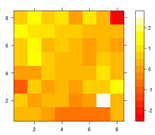
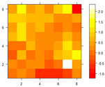
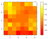
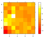
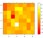
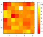
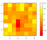
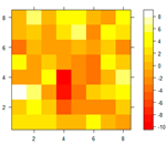
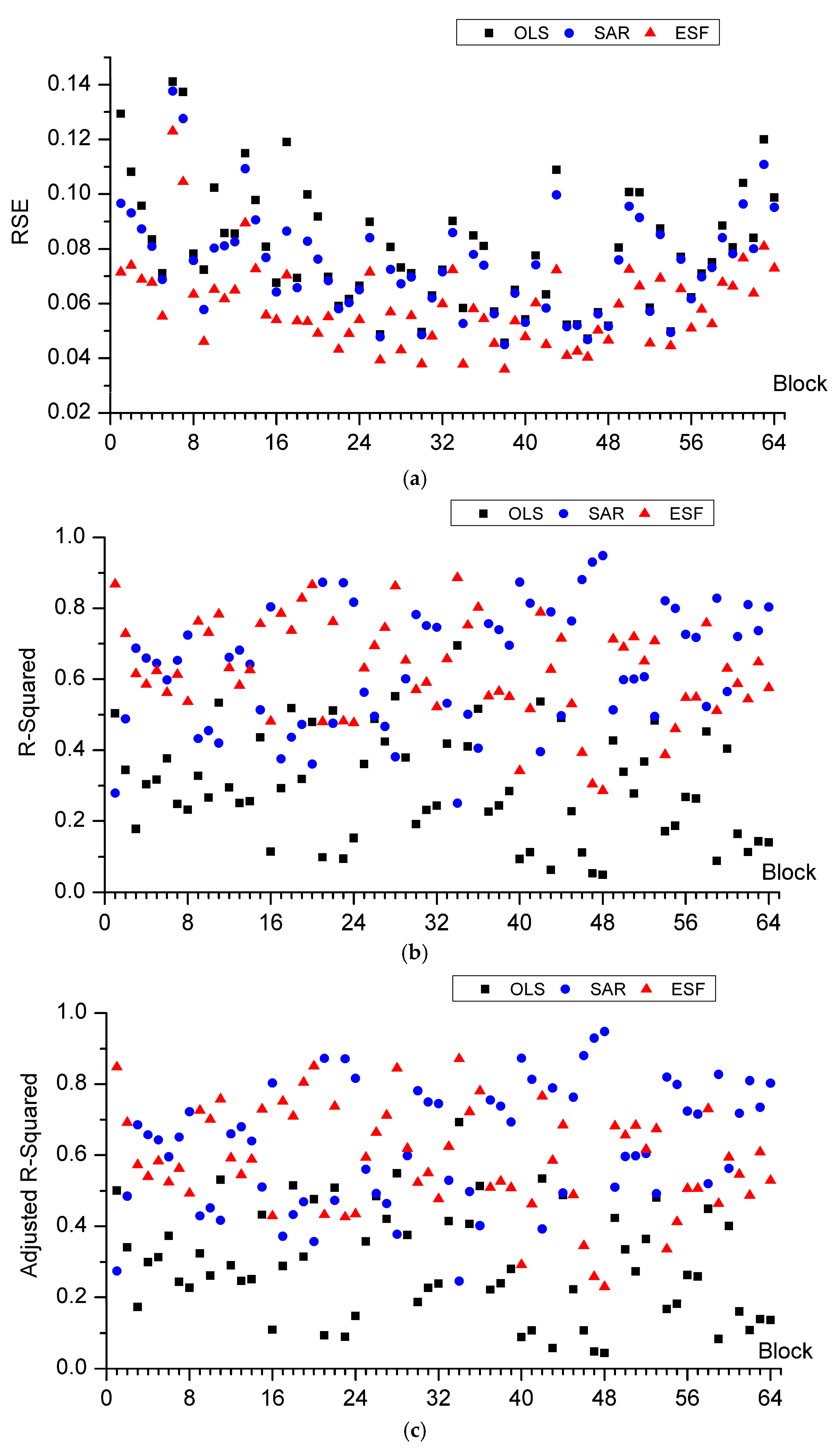
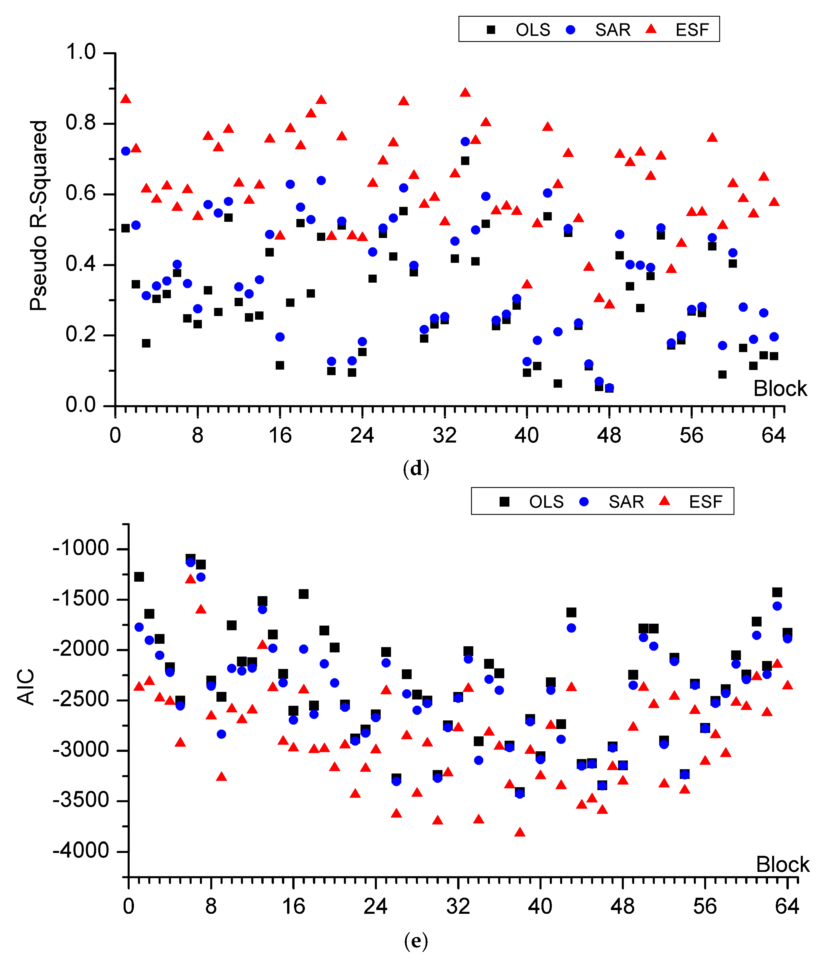
Criteria of OLS, SAR, and ESF for the segmented raster image blocks are computed to validate the goodness of fit for the three models as 
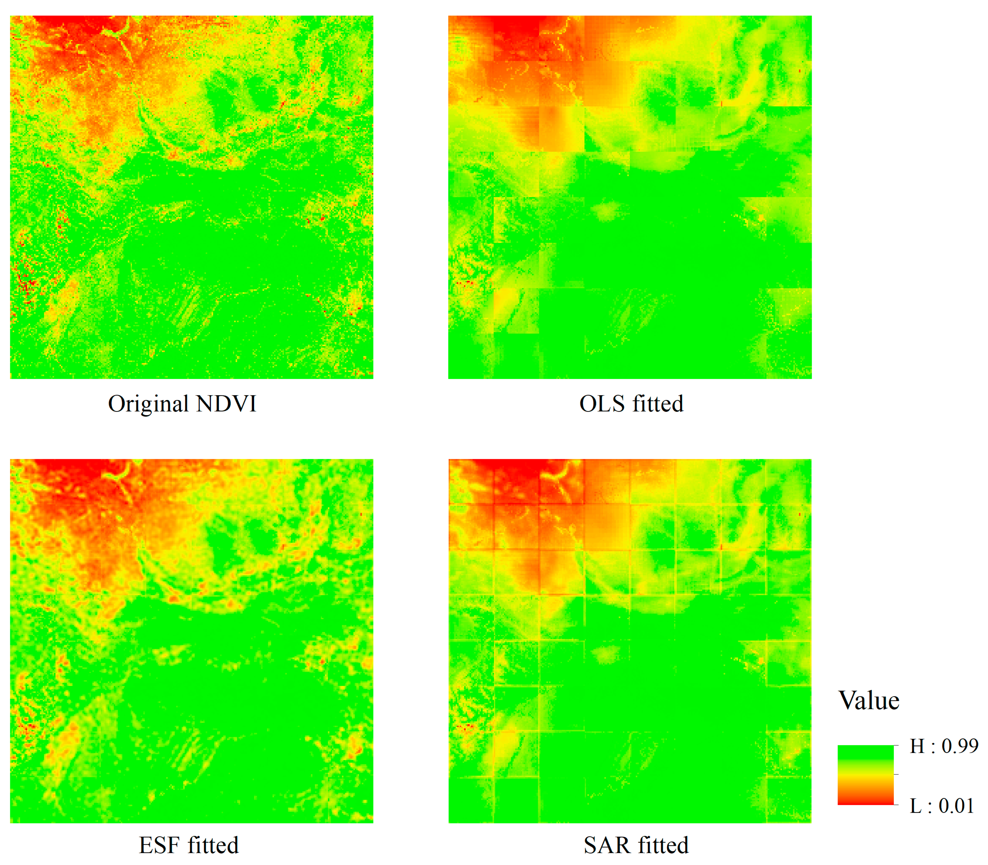
Figure 4 shows. The RSE of ESF model is smaller than SAR and much smaller than OLS model. ESF model almost gets the minimum RSE value among the three models, which means less difference between observed value and predicted value. R-Squared of both ESF model and SAR model is greater than OLS model, mainly because of the filtered eigenvectors and spatial interaction component explaining the spatial effects in the regression model. For some blocks, the R-Squared of SAR is greater than ESF, while in other blocks it is the opposite. Considering the spuriously increasing effects by adding extra explanatory variables to the model, Adjusted R-Squared are calculated to modify R-Squared. Adjusted R-Squared of ESF decrease a little bit compared to the other two models, due to a set of synthetic proxy variables, the filtered eigenvectors, being added to the explanatory variables. For R-Squared and Adjusted R-Squared, it is hard to say whether SAR is better than ESF or not. However, what is certain is that both of the R-Squared and Adjusted R-Squared show an increased proportion of the dependent variable that can be explained by explanatory variables of regression model. Pseudo R-Squared for the 3 models are calculated, which can measure the goodness of fit between fitted values and observed values. It is obvious that ESF model gets the greatest value in all blocks. AIC of the three models are compared, which takes both model complexity and goodness of fit into consideration. Lower AIC represents better model. ESF model gets the smallest AIC, while OLS gets the greatest AIC in all blocks. Considering all these criteria, ESF and SAR models are much better than OLS, owing to their consideration of spatial dependent component. ESF model is better than SAR model for its better fit and relative high comprehensive comparison.

4.2. Summarized Results

Table 5 summarizes criterion of the three models by calculating mean of parameters from the segmented blocks. Due to the variations of ESFs in ESF model, only coefficients of environmental factors are calculated for global ESF model.
The coefficients estimated for explanatory variables vary in the three models. For DEM, the average estimated coefficients of the three models are similar, together with a similar standard error average. The p value for SAR and ESF models is less than 0.05, which means a significant relationship under 95% confidence level. For PREC, the coefficient estimates for OLS model and SAR model are similar and greater than ESF model. The average standard error for ESF is better than the other two models. The p values for PREC of the three models are all greater than 0.05, representing no significance.
For RHU and DAYP, ESF model produces the largest slope value among all three models but gets a higher standard error for estimated coefficients. The p values are similar and not significant. For OC, the estimated coefficients show difference, while the standard errors of SAR and ESF models decrease. The p values of the three models for BS are not significant. Residuals’ MC is an indicator to detect spatial autocorrelation in residuals. The smaller residuals’ MC means more spatial structure components are interpreted by regression model. The residuals’ MC for SAR model decreases compared to OLS model, but for ESF it decreases nearly to excepted level ( E ( M C ) = 1 n 1 = 9.78 × 10 4 ). The p values of residuals’ MC for OLS and SAR are significant but no more significant for ESF.
Table 6 shows the parameter estimation result in Block Group 35 randomly selected. There are several differences between the average of all blocks and Block 35. The estimated coefficient for DAYP is much larger in Block 35. The p value of estimated coefficients for all three models is significant, except for OC in OLS and SAR, and RHU in ESF.
Criteria of all blocks are summarized to compare the parallel ESF model with OLS and SAR model. The RSE, R-Squared, Adjusted R-Squared, and Pseudo R-squared are recalculated from the estimated value and observed value. The mean of AIC value, Residuals’ MC, and degree of freedom (DF) are calculated. The results are shown in Table 7.
Compare the results from the table, what the integrated results show is in accordance with the segmented results. The RSE of SAR model is smaller than OLS and for ESF is much smaller, which shows less difference between fitted values and observed values using the SAR model and ESF model. Residuals’ MC is an indicator to detect spatial autocorrelation in residuals. It is obvious that ESF is much more effective than the other two models. R-Squared of SAR model and ESF model increases compared to OLS model. These environmental factors explain only 30% of the variation in NDVI, while spatial autocorrelation captured by ESF term explains addtional 30%. This is mainly because new variables that explain spatial effects are added to global ESF model. Considering the automatically and spuriously increasing effect by adding extra explanatory variable to regression model, Adjusted R-Squared of ESF model decreases slightly, because its number of variables is more than the other two models. The average DF is calculated, representing good performance for OLS and SAR. Pseudo R-Squared is also calculated, which can reflect the goodness of fit between observed values and fitted values. It is obvious than ESF model is better than SAR and much better than OLS. Taking both model complexity and goodness of fit into consideration, AIC gives the best choice. AIC for ESF is smaller than SAR and much smaller than OLS. Considering all these criteria, it is obvious that ESF is relatively better than SAR and much better than OLS.

4.3. Time Cost Comparison in Parallel Computation

In this study, parallel computation based on different clusters of different number of cores is conducted to verify the speed-up ratio. The experiment is conducted on an ordinary PC configured with 4 cores in total. The time cost of parallel computation on different number of workers is shown as Table 8. It is obvious that the calculation procedure can be accelerated dramatically by adding workers to cluster; cluster with 4 workers can be 3.2 times faster than cluster with only one worker or serial computation.

5. Discussion

In this study, a parallel ESF regression approach for large size raster datasets of NDVI and its environmental factors based on segmentation is proposed to solve the problem of inaccuracy and uncertainty for regression model caused by spatial autocorrelation and insufficiency of calculating ability for large size raster datasets. The influence of environmental factors and spatial effects to NDVI in central China is discussed by OLS, SAR, and proposed parallel ESF model.

5.1. Influence for NDVI Distribution

The correlation coefficient in Table 3 shows the correlation of variables for the whole region. However, the performance in the segmented blocks is not necessarily the same with the whole data. Strong positive correlations between NDVI and metrological factors (precipitation, humidity, and precipitation days) are not that strong and are even negative in some segmented blocks. The p values of estimated coefficient for OLS of the whole region are less than 0.05, and statistical significant, but insignificant p values exist in some segmented blocks. Therefore, the number of blocks whose p-value is less than 0.05 in all blocks is counted to see the performance of environmental variables in each segmented blocks. The percentage of these blocks is also calculated as Table 9 shows.
From Table 9, the percentage of environmental variables whose p value for coefficient estimation is similar among the three models, except for PREC and BS in ESF model, which is less than 50%. Table 10 shows the estimated coefficients for all blocks using the OLS, SAR, and ESF models. Cells in images represent the estimated coefficients of the block corresponding to the site. A red cell stands for a higher value of estimated coefficient. From the table, OLS and SAR models portray similar distribution for environmental variables, while the ESF model displays a slightly different distribution. Both of the high values and low values estimated by the three models for each variable almost have similar distributions.

5.2. Implementation of Parallel ESF

Parallel ESF regression model is proposed by image segmentation. The segmentation of large raster datasets to smaller ones with the same size of 32 × 32 provides a feasible approach to solve the incapable computation of ESF for large raster datasets limited by the computing power of computers. The eigenvectors spatial filtering procedure can be accelerated remarkably by parallel computation based on multi-core cluster. Figure 5 shows fitted images for the three models fitted values. The parallel ESF regression model performs closest to the original NDVI and presents the most similar characteristics compared with the other two models. Although SAR model is fitted similarly to the original image, the boundary pixels of each segmented block present obvious differences, which look like lines segmenting the whole image. OLS model is fitted the worst, both in terms of integrality and goodness of fit.

5.3. Drawback

A drawback is that there is no consideration of the contiguity of border pixels between segmented blocks. The accuracy of regression analysis might have been affected by the isolation between blocks from segmentation, which may have influenced the estimation of the fitted dependent variable for the border pixels. Although the influence has not been evaluated, it is likely that the error would decrease if additional rows and columns included in the segmented blocks. The study of this issue will be continued in future works.

6. Conclusions

In this study, the influence of environmental factors and spatial effects on vegetation cover in central China are studied. A parallel ESF regression model based on raster segmentation is proposed for regression analysis of large, regular-squared raster datasets and applied to NDVI and its factors of DEM, PREC, RHU, DAYP, OC, and BS. The influences on NDVI distribution are studied that regional effects can influence the correlation relation between NDVI and environmental variables. The result shows that goodness of fit for the parallel ESF model is greatest compared to the conventional OLS model and the SAR model. Moreover, spatial effects account for nearly 32% variation for NDVI distribution. By using the proposed parallel ESF regression approach, a more accurate model is constructed for NDVI and its environmental factors in central China. That is to say, spatial effects, especially spatial autocorrelation, plays an important role in vegetation cover distribution in central China. Despite the filtered eigenvectors added to regression model that cause an increase of model complexity, the parallel ESF model still has the best goodness of fit and the best performance by criteria as R-Squared, Adjusted R-Squared, Pseudo R-Squared, and AIC, interpreting spatial autocorrelation and improving the goodness of fit.
The ESF approach can account for influence caused by spatial autocorrelation and improve the degree of fitting, but it produces no results for large size rasters because of the calculation bottleneck of eigenvector generation and eigenvector selection. In this study, the parallel approach is proposed for the long-consuming stepwise process for large size eigenvectors derived from SWM responding to spatial relation among pixels in the raster image. The large datasets are segmented to smaller ones and distributed to a multi-core cluster for parallel computation of eigenvector spatial filtering in each segmented block, which can be extended to a cluster with more cores to improve the computing speed for much larger datasets. The parallel technique for ESF regression provides a feasible approach to solve the problem of inaccuracy and uncertainty caused by spatial autocorrelation in regression analysis for large raster datasets and computational burdens of the eigenvector spatial filtering algorithm, which can be used not only in NDVI analysis but also to construct more accurate regression models for variables of large size raster datasets, which is very promising for applying spatial regression modeling to a wide range of real world problem solving and forecasting.

Author Contributions

Conceptualization, J.Y. and Y.C.; Data curation, M.C. and F.Y.; Formal analysis, M.C., F.Y. and M.Y.; Methodology, J.Y. and Y.C.; Resources, J.Y.; Software, J.Y. and M.Y.; Validation, J.Y.; Writing—original draft, J.Y.; Writing—review & editing, Y.C.

Funding

This research was funded by [the National Key S&T Special Projects of China] grant number (2017YFB0503704) and [the National Nature Science Foundation of China] grant numbers (41671380, 41531180).

Acknowledgments

This research was funded by [the National Key S&T Special Projects of China] grant number (2017YFB0503704) and [the National Nature Science Foundation of China] grant numbers (41671380, 41531180). The authors sincerely acknowledge their financial support for this research.

Conflicts of Interest

The authors declare no conflict of interest.

References

  1. Rouse, J.W. Monitoring vegetation systems in the Great Plains with ERTS. NASA Spec. Publ. 1974, 351, 309. [Google Scholar]
  2. Pettorelli, N.; Vik, J.O.; Mysterud, A.; Gaillard, J.M.; Tucker, C.J.; Stenseth, N.C. Using the satellite-derived ndvi to assess ecological responses to environmental change. Trends Ecol. Evol. 2005, 20, 503–510. [Google Scholar] [CrossRef] [PubMed]
  3. Nicholson, S.E.; Farrar, T.J. The influence of soil type on the relationships between ndvi, rainfall, and soil-moisture in semiarid Botswana. I. Ndvi response to rainfall. Remote Sens. Environ. 1994, 50, 107–120. [Google Scholar] [CrossRef]
  4. Di, L.P.; Rundquist, D.C.; Han, L.H. Modeling relationships between ndvi and precipitation during vegetative growth cycles. Int. J. Remote Sens. 1994, 15, 2121–2136. [Google Scholar] [CrossRef]
  5. Chamailléjammes, S.; Fritz, H. Precipitation-ndvi relationships in eastern and southern African savannas vary along a precipitation gradient. Int. J. Remote Sens. 2009, 30, 3409–3422. [Google Scholar] [CrossRef]
  6. Padmanaban, R.; Bhowmik, A.K.; Cabral, P. A remote sensing approach to environmental monitoring in a reclaimed mine area. Int. J. Geo-Inf. 2017, 6, 401. [Google Scholar] [CrossRef]
  7. Schultz, P.A.; Halpert, M.S. Global correlation of temperature, ndvi and precipitation. Adv. Space Res. 1993, 13, 277–280. [Google Scholar] [CrossRef]
  8. An, C.; Fan, J.; Zhang, Y.; Yan, D. Characterizing the responses of vegetation to climate change in the Tibet Plateau using remote sensing data. J. Appl. Remote Sens. 2018, 12, 016035. [Google Scholar] [CrossRef]
  9. Guo, H.; Lei, L. Vegetation greenness trend (2000 to 2009) and the climate controls in the Qinghai-Tibetan Plateau. J. Appl. Remote Sens. 2013, 7, 3572. [Google Scholar]
  10. Hou, W.; Gao, J.; Wu, S.; Dai, E. Interannual variations in growing-season ndvi and its correlation with climate variables in the southwestern karst region of China. Remote Sens. 2015, 7, 11105–11124. [Google Scholar] [CrossRef]
  11. Griffith, D.A. Positive spatial autocorrelation impacts on attribute variable frequency distributions. Chil. J. Stat. 2011, 2, 3–28. [Google Scholar]
  12. Griffith, D.; Chun, Y. Spatial autocorrelation and uncertainty associated with remotely-sensed data. Remote Sens. 2016, 8, 535. [Google Scholar] [CrossRef]
  13. Iwasaki, H. Ndvi prediction over mongolian grassland using gsmap precipitation data and jra-25/jcdas temperature data. J. Arid. Environ. 2009, 73, 557–562. [Google Scholar] [CrossRef]
  14. Chen, Y.; Zhou, J.; Wilson, J.P.; Wu, J.; Wu, Q.; Yang, J. A dynamic classification pattern of spatial statistical services using formal concept analysis. Geogr. Anal. 2018. [Google Scholar] [CrossRef]
  15. Burden, S.; Cressie, N.; Steel, D.G. The SAR model for very large datasets: A reduced rank approach. Econometrics 2015, 3, 317–338. [Google Scholar] [CrossRef]
  16. Griffith; Daniel, A. Spatial Statistics & Geostatistics; Sage: Newcastle upon Tyne, UK, 2013; pp. 314–322. [Google Scholar]
  17. Griffith, D.A.; Paelinck, J.H.P. An equation by any other name is still the same: On spatial econometrics and spatial statistics. Ann. Reg. Sci. 2007, 41, 209–227. [Google Scholar] [CrossRef]
  18. Griffith, D.A. Spatial autocorrelation and eigenvectors of the geographic weights matrix accompanying geo-referenced data. Can. Geogr. 1996, 40, 351–367. [Google Scholar] [CrossRef]
  19. Chun, Y.; Griffith, D.A.; Lee, M.; Sinha, P. Eigenvector selection with stepwise regression techniques to construct eigenvector spatial filters. J. Geogr. Syst. 2016, 18, 67–85. [Google Scholar] [CrossRef]
  20. Griffith, D.A.; Paelinck, J.H.P. Non-Standard Spatial Statistics and Spatial Econometrics; Springer Science & Business Media: Berlin, Germany, 2011. [Google Scholar]
  21. Patuelli, R.; Griffith, D.A.; Tiefelsdorf, M.; Nijkamp, P. The use of spatial filtering techniques: The spatial and space-time structure of german unemployment data. SSRN Electron. J. 2006. [Google Scholar] [CrossRef]
  22. Griffith, D.A.; Peres-Neto, P.R. Spatial modeling in ecology: The flexibility of eigenfunction spatial analyses. Ecology 2006, 87, 2603–2613. [Google Scholar] [CrossRef]
  23. Xiao, Y.; Chen, X.; Li, Q.; Yu, X.; Chen, J.; Guo, J. Exploring determinants of housing prices in Beijing: An enhanced hedonic regression with open access poi data. Int. J. Geo-Inf. 2017, 6, 358. [Google Scholar] [CrossRef]
  24. Griffith, D.A. Eigenfunction properties and approximations of selected incidence matrices employed in spatial analyses. Linear Algebra Appl. 2000, 321, 95–112. [Google Scholar] [CrossRef]
  25. Lovell, J.L.; Graetz, R.D. Filtering pathfinder avhrr land ndvi data for Australia. Int. J. Remote Sens. 2001, 22, 2649–2654. [Google Scholar] [CrossRef]
  26. Geerken, R.; Zaitchik, B.; Evans, J.P. Classifying rangeland vegetation type and coverage from ndvi time series using fourier filtered cycle similarity. Int. J. Remote Sens. 2005, 26, 5535–5554. [Google Scholar] [CrossRef]
  27. Mccallum, Q.E.; Weston, S. Parallel R; O’Reilly Media, Inc.: Newton, MA, USA, 2011. [Google Scholar]
  28. Zhao, P. R with parallel computing from user perspectives. In Parallel R; O’Reilly Media, Inc.: Newton, MA, USA, 2016; Volume 2016. [Google Scholar]
  29. Helbich, M.; Griffith, D.A. Spatially varying coefficient models in real estate: Eigenvector spatial filtering and alternative approaches. Comput. Environ. Urban 2016, 57, 1–11. [Google Scholar] [CrossRef]
  30. Griffith, D.A. Spatial Autocorrelation and Spatial Filtering: Gaining Understanding through Theory and Scientific Visualization; Springer Science & Business Media: Berlin, Germany, 2013. [Google Scholar]
  31. Tiefelsdorf, M.; Boots, B. The exact distribution of Moran’s I. Environ. Plan. A 2000, 27, 985–999. [Google Scholar] [CrossRef]
  32. Fischer, M.M.; Nijkamp, P. Handbook of Regional Science; Springer: Berlin/Heidelberg, Germany, 2014; pp. 1419–1434. [Google Scholar]
  33. Griffith, D.A. Spatial Autocorrelation and Spatial Filtering; Springer: Berlin/Heidelberg, Germany, 2013; pp. 633–635. [Google Scholar]
  34. Benesty, J.; Chen, J.; Huang, Y.; Cohen, I. Pearson correlation coefficient. In Noise Reduction in Speech Processing; Springer: New York, NY, USA, 2009; pp. 1–4. [Google Scholar]
  35. LeSage, J.P. An introduction to spatial econometrics. Rev. D’économie Industrielle 2008, 123, 19–44. [Google Scholar] [CrossRef]
  36. Ward, M.D.; Gleditsch, K.S. Spatial Regression Models; Sage: Newcastle upon Tyne, UK, 2008; Volume 155. [Google Scholar]
  37. Wikipedia. Hunan#geography. Available online: https://en.wikipedia.org/wiki/Hunan#Geography (accessed on 28 July 2014).
  38. Chenghu, Z.; Weimin, C. 1:1 Million Digital Geomorphologic Data Sets in Western China; Environmental and Ecological Science Data Center for West China, National Natural Science Foundation of China: Beijing, China, 2007. [Google Scholar]
  39. Domrös, M.; Gongbing, P. The Climate of China; Springer: New York, NY, USA; Berlin, Germany, 2011; pp. 265–266. [Google Scholar]
  40. Fu, C.; Jiang, Z.; Guan, Z.; He, J.; Xu, Z. Regional Climate Studies of China; Springer: Berlin/Heidelberg, Germany, 2008. [Google Scholar]
  41. Defries, R.; Townshend, J. Ndvi-derived land cover classification at global scales. Int. J. Remote Sens. 1994, 15, 3567–3586. [Google Scholar] [CrossRef]
  42. Piao, S.; Fang, J.; Zhou, L.; Guo, Q.; Henderson, M.; Ji, W.; Li, Y.; Tao, S. Interannual variations of monthly and seasonal normalized difference vegetation index (ndvi) in China from 1982 to 1999. J. Geophys. Res. Atmos. 2003, 108. [Google Scholar] [CrossRef]
  43. Reuter, H.I.; Nelson, A.; Jarvis, A. An evaluation of void-filling interpolation methods for srtm data. Int. J. Geogr. Inf. Sci. 2007, 21, 983–1008. [Google Scholar] [CrossRef]
  44. Jobbagy, E.G.; Jackson, R.B. The vertical distribution of soil organic carbon and its relation to climate and vegetation. Ecol. Appl. 2008, 10, 423–436. [Google Scholar] [CrossRef]
  45. Ruggiero, P.G.C.; Batalha, M.A.; Pivello, V.R.; Meirelles, S.T. Soil-vegetation relationships in cerrado (Brazilian Savanna) and semideciduous forest, Southeastern Brazil. Plant Ecol. 2002, 160, 1–16. [Google Scholar] [CrossRef]
  46. Fischer, G.; Nachtergaele, F.; Prieler, S.; Van Velthuizen, H.; Verelst, L.; Wiberg, D. Global Agro-Ecological Zones Assessment for Agriculture (GAEZ 2008); IIASA: Laxenburg, Austria; FAO: Rome, Italy, 2008; Volume 10. [Google Scholar]
Figure 1. An illustration of image segmentation. (The large datasets are segmented to smaller ones with the size N × N. The optimum N is determined by tests of linear ESF for a single small block.).
Ijgi 07 00330 g001
Figure 2. The study area and NDVI distribution (NDVI is from monthly compositing dataset of MODIS Terra (MODND1D) in August 2009, which takes the maximum from 1 August to 1 September in 2009. The datasets are provided by International Scientific & Technical Data Mirror Site, Computer Network Information Center, Chinese Academy of Sciences. Projection Coordinate System: WGS 1984 UTM Zone 48N).
Ijgi 07 00330 g002
Figure 3. Raster data after preprocessed (DEM dataset was released in 2008, PREC, RHU, and DAYP datasets are yearly value of 2009, and OC and BS datasets were released in 2008).
Ijgi 07 00330 g003
Figure 4. (a) Comparison of RSE between OLS, SAR, and ESF; (b) comparison of R-Squared between OLS, SAR, and ESF; (c) comparison of Adjusted R-Squared between OLS, SAR, and ESF; (d) comparison of Pseudo R-Squared between OLS, SAR, and ESF; (e) comparison of AIC between OLS, SAR, and ESF. The X-axis means the serial number of segmented blocks by column.
Ijgi 07 00330 g004aIjgi 07 00330 g004b
Figure 5. Original NDVI image and fitted NDVI image of the three models.
Ijgi 07 00330 g005
Table 1. The details of original data sets for study area.
VariableMeaningResolutionRaster SizeSource
NDVIassess the cover level of green vegetation on the earth surface1 km848 × 848 pixelsMODIS/Terra
DEMa digital representation of ground-surface topography or terrain90 m6001 × 6001 pixelsSTRM
PRECthe total quantity of rainfall to the ground at a site within a year, which supplies most of the water that plants need to absorb1 km848 × 848 pixelsMeteorological Stations
RHUmoisture in the atmosphere, which influences the exchange of water between plants and atmosphere1 km848 × 848 pixelsMeteorological Stations
DAYPthe number of days for daily precipitation ≥ 0.1 mm1 km848 × 848 pixelsMeteorological Stations
OCa good indicator to access health condition of the soil, a good criterion for soil fertility30 arc seconds601 × 601 pixelsHDWS
BStotal ratio of exchangeable cations (nutrients) Na, Ca, Mg, and K. Access the capacity of absorbing nutrients in the soil30 arc seconds601 × 601 pixelsHDWS
Note: PREC standard for sum of precipitation of the year 2009. HUMI is abbreviation of average relative humidity of the year 2009. DAYP is abbreviation for number of daily precipitations more than 0.1 mm. PREC, RHU, and DAYP image data are interpolated from 555 surface meteorological stations within and around the study area by Kriging method under WGS-84 Coordinate System.
Table 2. Stepwise regression for variable selection results. All criteria calculated here are from global observations of the whole study area.
VariableβSEtStatp-ValueResidualRSERSquAdj.R2F-Statp-Value
MCp
Intercept0.150.0122.870.000.700.000.130.510.511148<2.2 × 10⁻¹⁶
DEM0.040.008.300.00
PREC0.480.0171.180.00
DAYP0.470.0138.470.00
RHU0.060.023.480.00
OC0.170.044.310.00
BS0.040.0014.850.00
Table 3. The correlation matrix among all variables.
NDVIDEMPRECRHUDAYPOCBS
NDVI1
DEM−0.261
PREC0.70−0.441
RHU0.66−0.360.851
DAYP0.62−0.010.810.821
OC0.070.170.070.080.191
BS−0.290.11−0.44−0.42−0.44−0.171
Table 4. Filtered eigenvectors (partly) and number of eigenvectors selected in each block.
Block No.Filtered EigenvectorsCounts
1 E V 6 , E V 2 , E V 8 , E V 3 , E V 33 , E V 11 , , E V 77 , E V 207 , E V 74 , E V 39 129
2 E V 32 , E V 5 , E V 17 , E V 21 , E V 9 , E V 23 , , E V 107 , E V 33 , E V 98 , E V 106 113
3 E V 1 , E V 14 , E V 24 , E V 16 , E V 10 , E V 17 , , E V 210 , E V 89 , E V 8 , E V 5 94
4 E V 3 , E V 32 , E V 17 , E V 10 , E V 14 , E V 45 , , E V 72 , E V 123 , E V 64 , E V 90 95
……
63 E V 1 , E V 15 , E V 9 , E V 12 , E V 6 , E V 5 , , E V 59 , E V 175 , E V 150 , E V 84 98
64 E V 2 , E V 7 , E V 14 , E V 4 , E V 13 , E V 38 , , E V 215 , E V 10 , E V 114 , E V 49 95
Table 5. Parameter estimate (mean) for the three models.
VariableOLSSARESF
βSEtStatp-ValueResidualβSEzp-ValueResidualβSEtStatp-ValueResidual
MCpMCpMCp
Intercept0.430.172.960.070.310.000.370.172.650.140.200.000.260.221.980.13−0.090.93
DEM0.360.096.410.070.370.085.850.050.350.094.660.04
PREC0.430.182.470.110.450.172.130.140.200.240.150.23
RHU0.010.270.010.16−0.020.26−0.300.110.280.360.410.12
DAYP0.320.361.330.120.210.341.150.120.460.481.670.13
OC0.560.990.820.210.330.930.580.200.650.840.730.20
BS0.010.030.010.220.010.02−0.010.260.020.020.520.26
Notes: Parameter estimate in this table is calculated by mean of the parameters from the 64 groups of image blocks. β is the estimated coefficient value of explanatory variables. SE is abbreviation for standard error of the estimate. The parameter tStat is t-statistic for a test that the coefficient is zero. MC is the Moran Coefficient of residuals and p is p-value for residuals’ MC.
Table 6. Parameter estimate for the three models in Block Group 35.
VariableOLSSARESF
βSEtStatp-ValueResidualβSEzp-ValueResidualβSEtStatp-ValueResidual
MCpMCpMCp
Intercept−1.060.11−9.610.000.390.00−0.050.11−4.790.000.230.000.660.135.230.00−0.110.98
DEM0.610.0610.680.000.330.066.040.000.250.083.150.00
PREC2.510.1220.500.001.590.1612.660.000.440.133.520.00
RHU2.440.317.980.003.050.2810.740.000.630.361.860.08
DAYP−8.160.50−16.220.00−7.950.46−17.180.00−6.200.73−8.490.00
OC1.311.540.850.390.911.410.650.522.671.292.080.04
BS0.110.042.850.000.080.042.300.020.070.032.290.02
Table 7. Summarized criteria of OLS, SAR, and ESF. The criteria here are calculated by observed value and fitted value of the model from the global observations.
CriteriaOLSSARESF
RSE0.15760.07460.0593
Residual’s MC0.310.2−0.09
R-Squared0.29930.63230.6268
Adjusted R-Squared0.29520.63010.5891
Pseudo R-squared0.300.370.63
DF10171017925
AIC (Akaike information criterion)−2234.94−2441.44−2847.47
Table 8. Time cost and speed up ratio of clusters containing different cores. The PC is equipped with Intel(R) Core(TM) i5-4590 CPU @ 3.30 GHz processor, 8.0 GB RAM, and Windows 10 Operating System.
Number of CoresTime Cost (Seconds)Speed-Up Ratio
14770.201
22621.021.8
41470.163.2
Table 9. Number of blocks and percentage whose p-value < 0.05 in all 64 blocks.
VariableOLSSARESF
NumberPercentNumberPercentNumberPercent
Intercept5382.81%4570.31%4367.19%
DEM5789.06%5585.94%5687.50%
PREC4976.56%4468.75%3148.44%
RHU4468.75%4468.75%4976.56%
DAYP4773.44%4062.50%4468.75%
OC3656.25%3453.13%3453.13%
BS3656.25%3453.13%2843.75%
Table 10. Image of estimated coefficients for OLS, SAR, and ESF models. The X and Y-axis represent the position of segmented datasets corresponding to the original large dataset.
OLSSARESF
DEM Ijgi 07 00330 i001 Ijgi 07 00330 i002 Ijgi 07 00330 i003
PREC Ijgi 07 00330 i004 Ijgi 07 00330 i005 Ijgi 07 00330 i006
RHU Ijgi 07 00330 i007 Ijgi 07 00330 i008 Ijgi 07 00330 i009
DAYP Ijgi 07 00330 i010 Ijgi 07 00330 i011 Ijgi 07 00330 i012
OC Ijgi 07 00330 i013 Ijgi 07 00330 i014 Ijgi 07 00330 i015
BS Ijgi 07 00330 i016 Ijgi 07 00330 i017 Ijgi 07 00330 i018

