A Methodology for Planar Representation of Frescoed Oval Domes: Formulation and Testing on Pisa Cathedral

 ,
,  ,
, 
Abstract
1. Introduction
- performing the development (more appropriately termed as projection and pseudo-development for non-directly developable surfaces) of geometric shapes;
- applying a reference system (u,v) to geometric shapes in order to retain their association with textures.
2. Materials
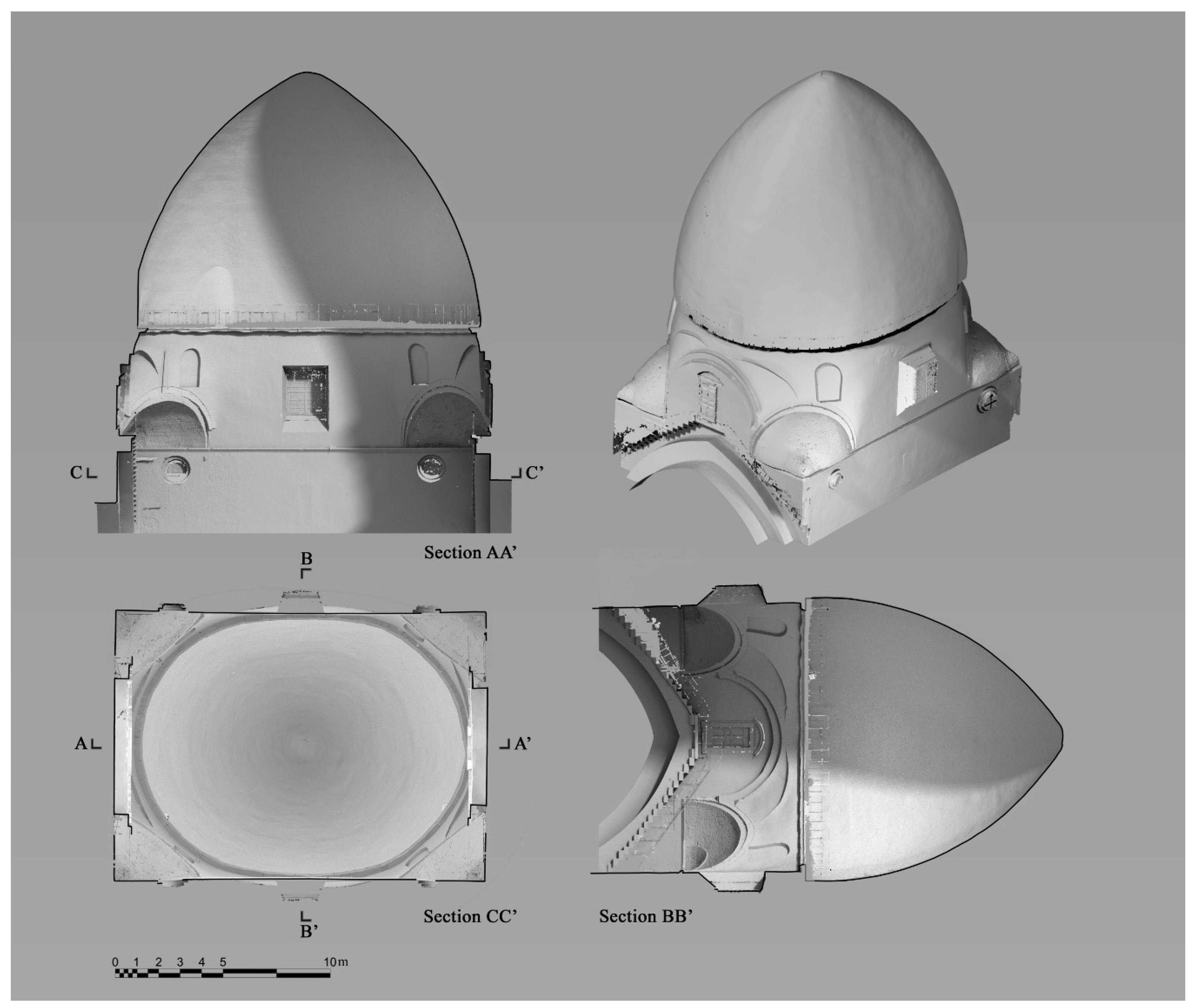
Surveying
- Topographical survey of a support network, at ground level.
- Laser scanning and photogrammetry of the intrados, at ground level.
- Laser scanning and photogrammetry of the intrados, at matroneum level.
- Topographical survey of an internal support network, at springer level.
- Laser scanning and photogrammetry of the intrados, at springer level.
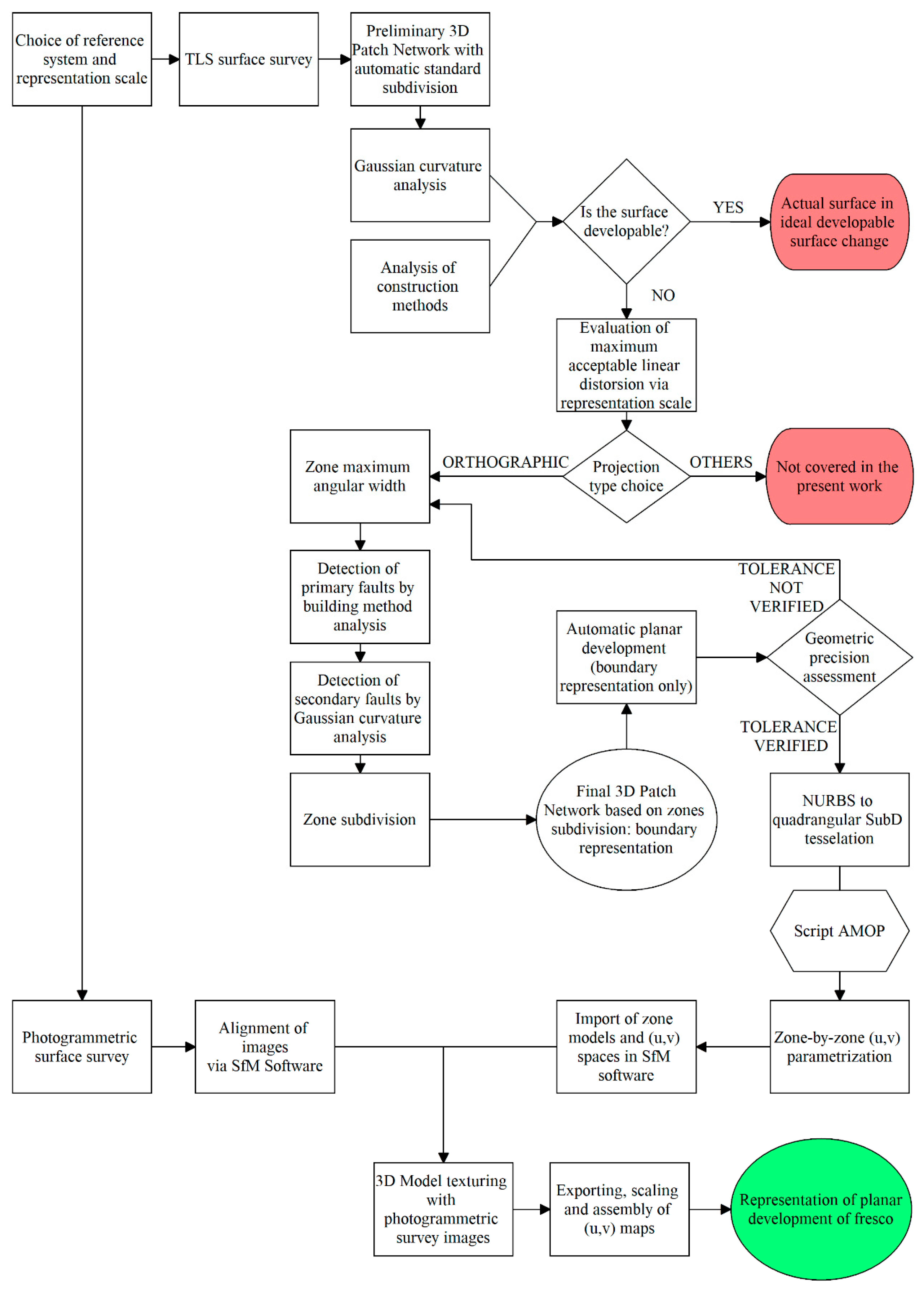
3. Methods
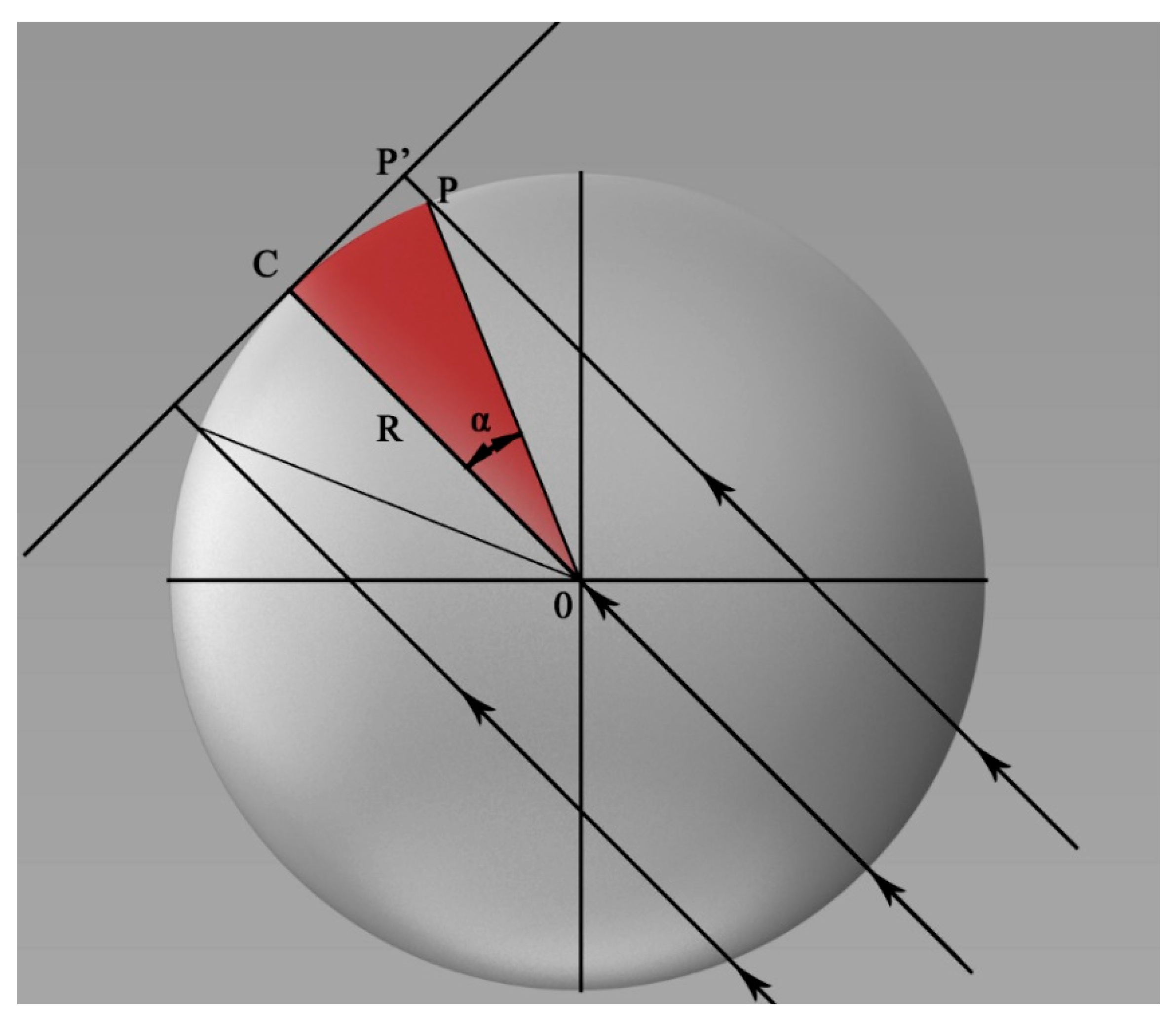
3.1. Geometry Pseudo-Development
- simple curvature surfaces: k1 = 0, k2 ≠ 0; or k1 ≠ 0, k2 = 0.
- double curvature surfaces: k1 ≠ 0, k2 ≠ 0.
- k > 0 define ellipsoids, which can be concave (k1 > 0 and k2 > 0) or convex (k1 < 0 and k2 < 0);
- k = 0 further distinguishes between k1 = k2 = 0 (plane) and either k1 or k2 ≠ 0 (cylinder);
- with k < 0, the two main curvatures have opposite signs, identifying a saddle surface.
3.2. Geometry Pseudo-Development
3.3. Design Analysis and Constructive Issues
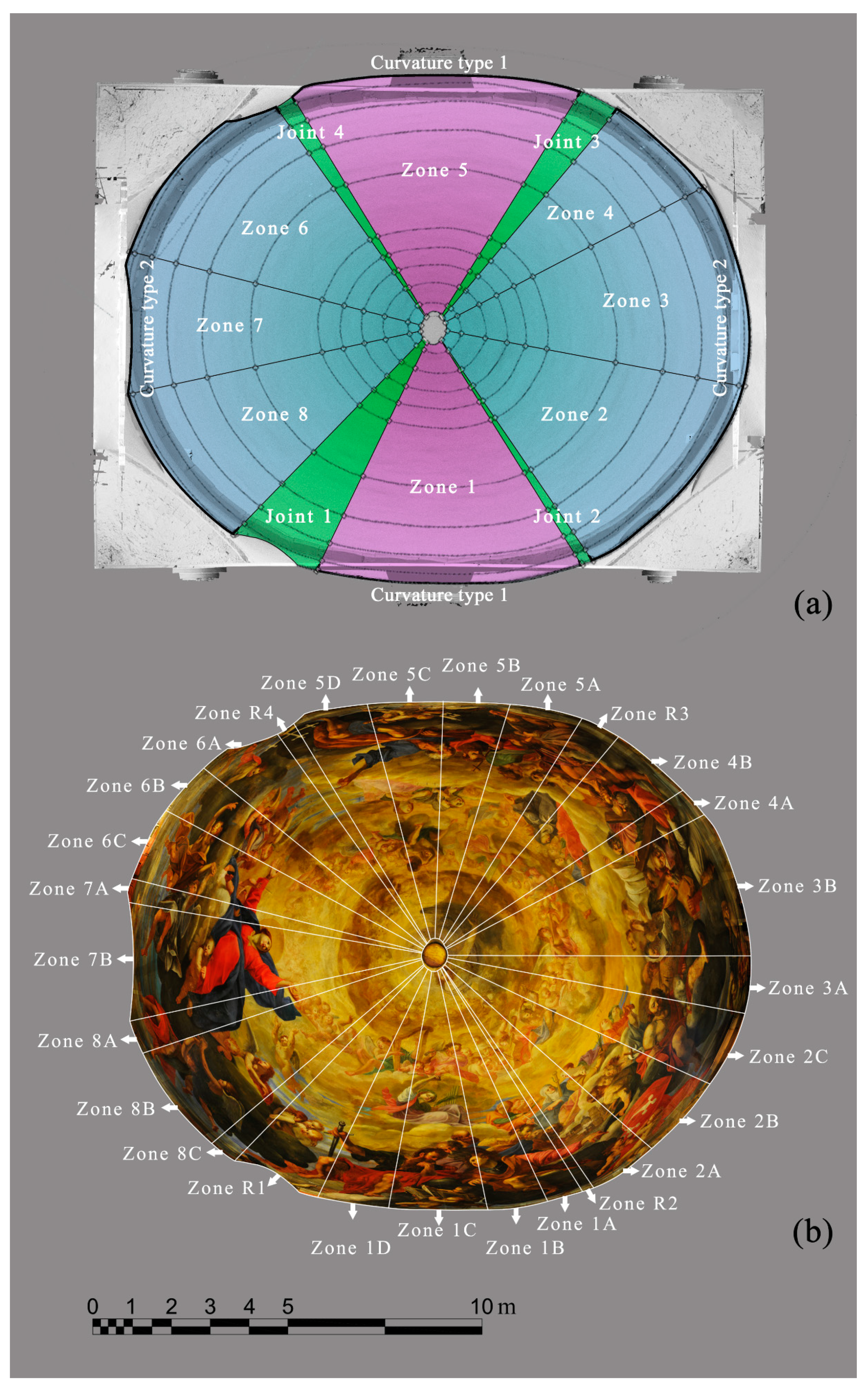
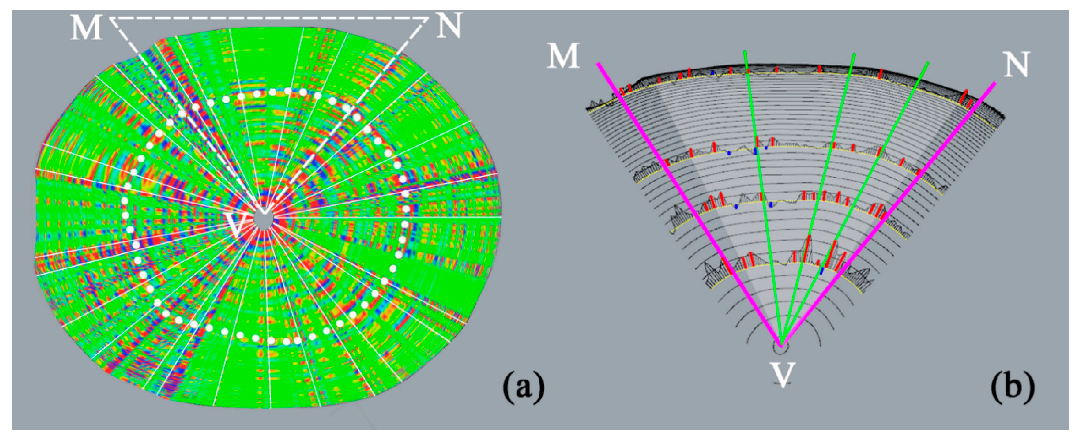
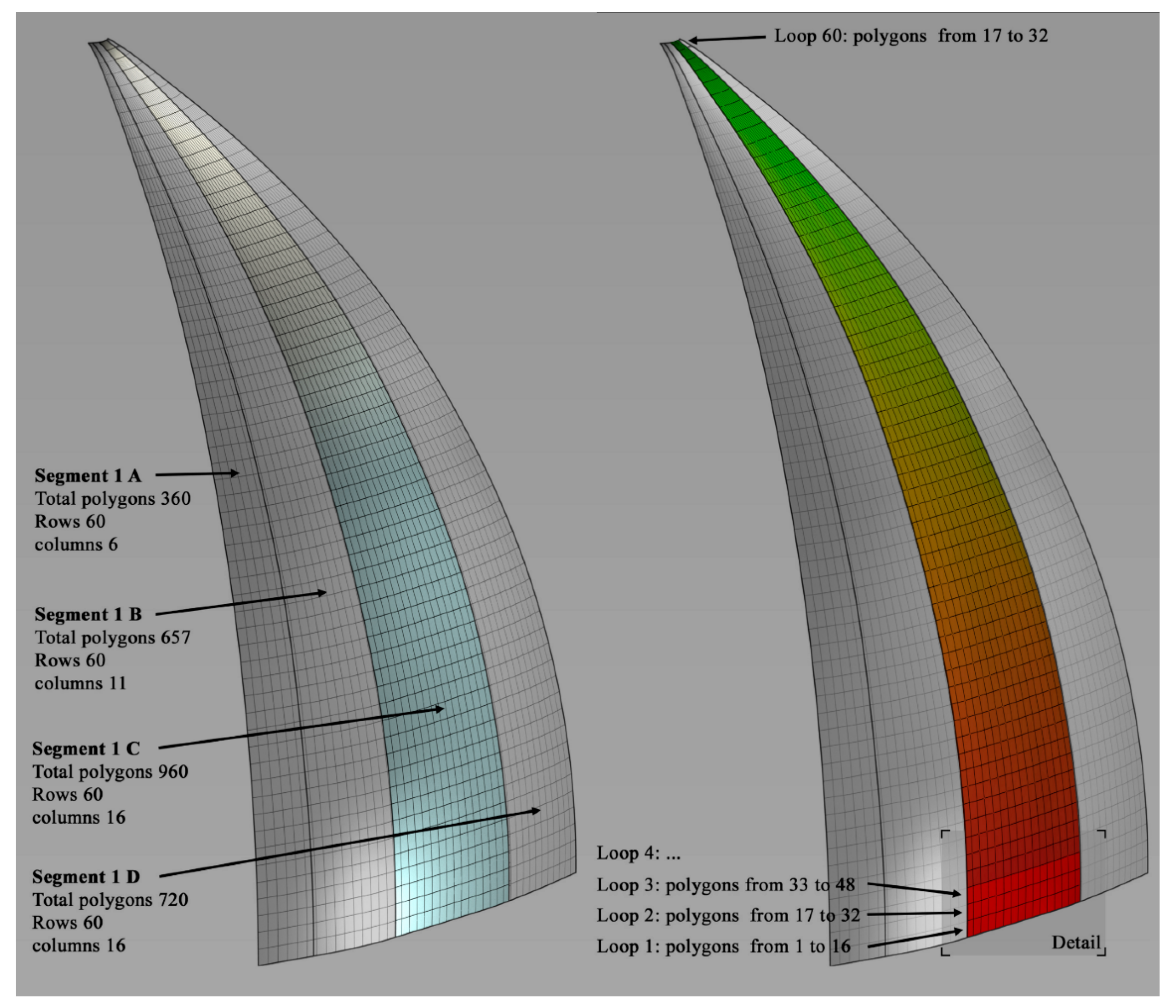
3.4. Segmentation of the Cupola
- identification in the macro-sector of positive “peaks” of the curvature (red color);
- identification of areas with low and constant curvature (blue);
- identification of inflection point areas (change from concave to convex, or vice versa): blue color abruptly alternated with red.
- Use of Rhinoceros to obtain the measurable surface for validation of the process and to determine whether it is developable or not. If it is not, a further partition of the piece is carried out according to the stated method.
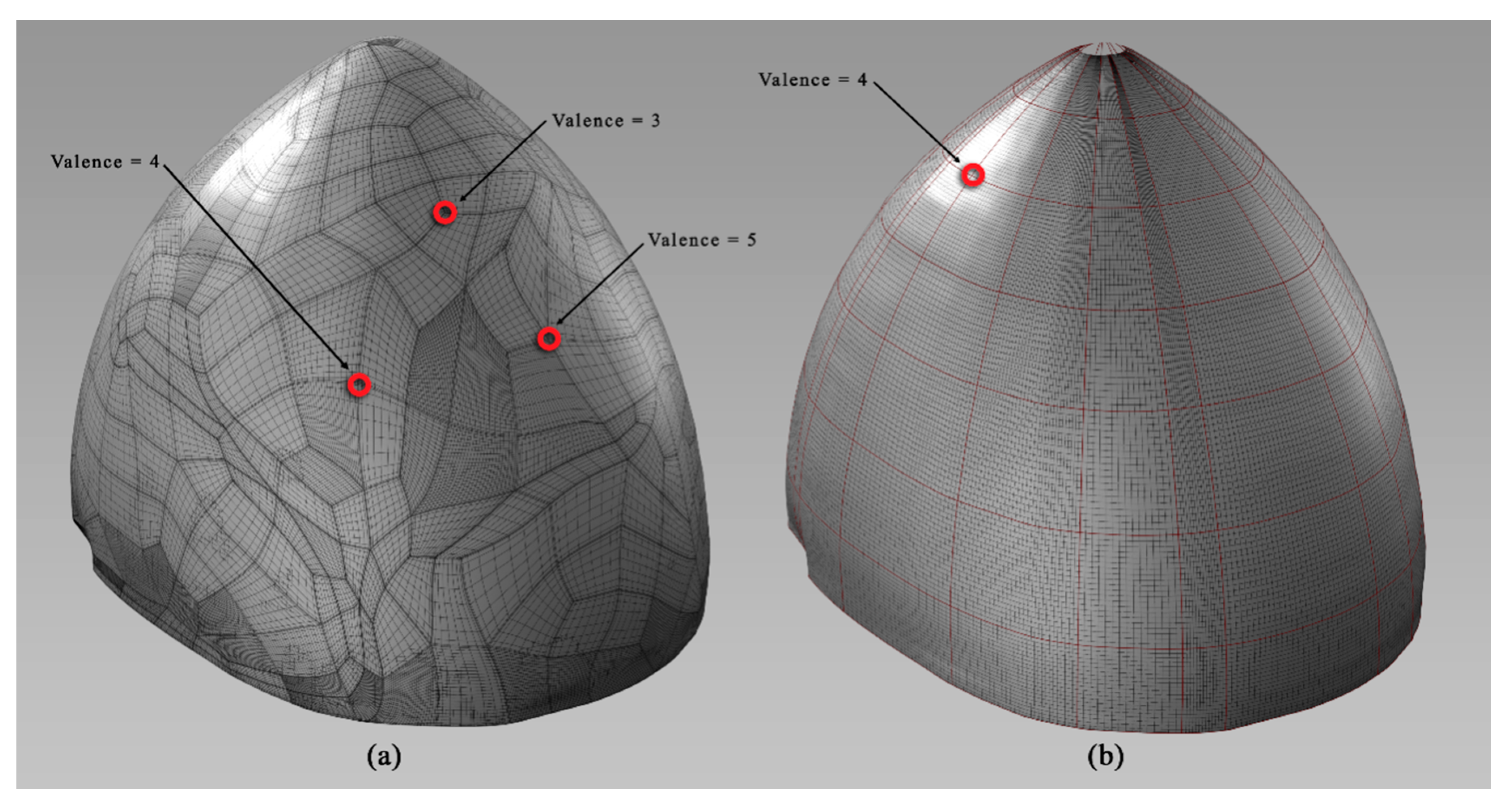
- Export of the single NURBS patches into a modeler equipped with a robust polygonal modeling kernel. The model is tessellated so as to maintain quadrangular topology, namely with all vertex valences equal to 4, with the only exception of the vertices forming part of the outer edge of the patch (valence equal to 2 or 3).
- Projection of each piece in the parameter space (u,v) through a script.
- Conversion of the (u,v) parameterized version into a mesh belonging to the reference system (x, y, z) and export towards NURBS modeling application.
- 2D polygon mesh conversion—obtained from parameterization—into NURBS model. This process takes place through the transformation of each cell (polygonal) of an equivalent patch (NURBS). This way, it will be possible to check the metric reliability of the projection operation.
- Model comparison and error evaluation— areas and lengths of the edges of the patch.
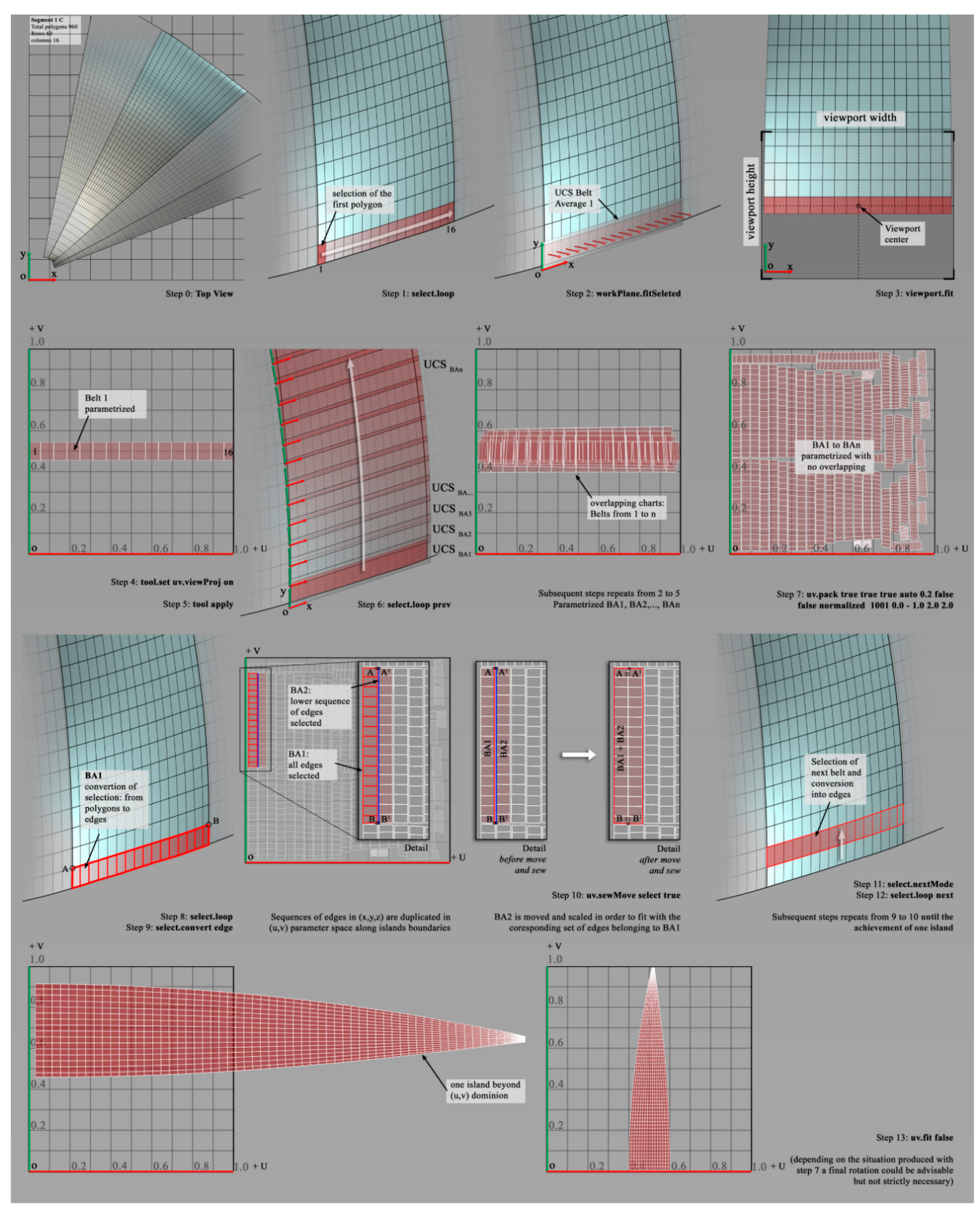
3.5. Automatic Multicenter Orthographic Projection (AMOP) Script
- 0.
- The necessary starting condition is that the model of each segment is displayed autonomously and in a single viewport, which must be strictly the orthographic view indicated with the name TOP (Top View). The first polygon in the lower left corner of the structured mesh of quadrangular polygons must be selected.
- 1.
- The script is launched, and it automatically selects the entire horizontal band of polygons (Belt 1): select.loop.
- 2.
- A drawing reference plane (UCS) is automatically set up; its normal vector is determined by the program through the average of the set of normals belonging to Belt 1, which we will call UCSBA1, i.e., UCS Belt Average 1: workPlane.fitSelect.
- 3.
- The initial TOP view (which allowed visualization of the segment from above) is now oriented in space in a congruent way with the normal outgoing from the plane defined by UCSBA1, which is centered on the selection together with the zoom value: viewport.fit.
- 4.
- A command is launched that makes a projection (central or parallel; in this case parallel) of the set of polygons selected in (x, y, z) onto the parameter space (u,v) using the view determined in the previous step: tool.setuv.viewProj on.
- 5.
- A one-to-one correspondence is established between the set of polygons of Belt 1 in (x, y, z) and an island in space (u,v): tool.apply.
- 6.
- The next band of polygons is automatically selected (Belt2): select.loop prev. From this point on, the sequence is repeated (Belt3, …, Beltn) until all the horizontal bands of polygons forming the segment are projected. These will appear superimposed in the parameter space (u,v) and therefore do not result as one-to-one correspondence with the whole set of points of the model in R3: a necessary and sufficient condition for correct texturing.
- 7.
- The biunique relationship is re-established by assigning ∀ Belt1, …, n a specific space in (u,v): uv.pack true false true auto 0.2 false false nearest 1001 0.0 −1.0 2.0 2.0.
- 8.
- The first polygon on the bottom left is selected by the user that launches the second script that selects the entire horizontal band of polygons (Belt 1): select.loop.
- 9.
- The selection of Belt 1 is converted from polygons into edges: select.convert edge.
- 10.
- The one-to-one correspondence between the bands in R3 (Belt1, …, n) and their counterparts in (u,v) is not verified along the edges of the single islands of the Belts. The outlines of the islands are partly duplicated (see image) since they will belong to the previous and the next band. Since the program highlights this duplication, it is possible to exploit it to automate the “stitching” of the adjacent belts through the command: uv.sewMove select true.
- 11.
- From here on, the script repeats the operation of the previous point, changing first the selection filter: select.NextMode.
- 12.
- The next band is selected: select.loop next.
- 13.
- Upon merging all the belts into one island, a fitting is necessary in order not to extend the patch beyond the boundaries of the (u,v) space: uv.fit false.
3.6. Associating Textures with Geometry Pseudo-Development
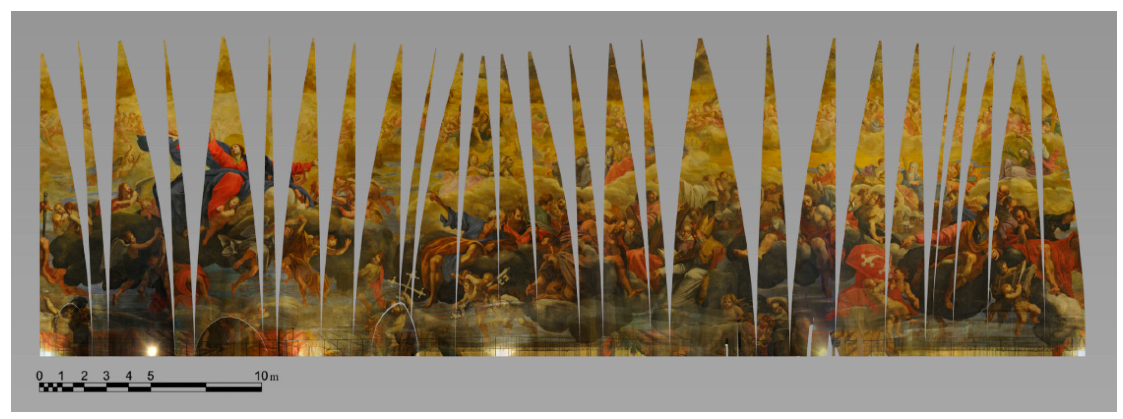
4. Results and Discussion
5. Conclusions
Author Contributions
Funding
Acknowledgments
Conflicts of Interest
References
- Robleda, P.G.; Caroti, G.; Martínez-Espejo Zaragoza, I.; Piemonte, A. Computational vision in UV-mapping of textured meshes coming from photogrammetric recovery: Unwrapping frescoed vaults. ISPRS Int. Arch. Photogramm. Remote Sens. Spat. Inf. Sci. 2016, XLI-B5, 391–398. [Google Scholar] [CrossRef]
- Caroti, G.; Martínez-Espejo Zaragoza, I.; Piemonte, A. Range and image based modelling: A way for frescoed vault texturing optimization. ISPRS Int. Arch. Photogramm. Remote Sens. Spat. Inf. Sci. 2015, XL-5/W4, 285–290. [Google Scholar] [CrossRef]
- Chiabrando, F.; Rinaudo, F. Recovering a collapsed medieval fresco by using 3D modeling techniques. ISPRS Ann. Photogramm. Remote Sens. Spat. Inf. Sci. 2014, II-5, 105–112. [Google Scholar] [CrossRef]
- Bevilacqua, M.G.; Caroti, G.; Piemonte, A.; Ruschi, P.; Tenchini, L. 3D survey techniques for the architectutal restoration: The case of St. Agata in Pisa. ISPRS Int. Arch. Photogramm. Remote Sens. Spat. Inf. Sci. 2017, XLII-5/W1, 441–447. [Google Scholar] [CrossRef]
- Clini, P.; Frontoni, E.; Quattrini, R.; Pierdicca, R. Augmented Reality Experience: From High-Resolution Acquisition to Real Time Augmented Contents. Adv. Multimed. 2014, 2014, 597476. [Google Scholar] [CrossRef]
- Sammartano, G.; Spanò, A. High scale 3D modelling and orthophoto of curved masonriesfor a multipurpose representation, analysis and assessment. ISPRS Int. Arch. Photogramm. Remote Sens. Spat. Inf. Sci. 2017, XLII-5/W1, 245–252. [Google Scholar] [CrossRef]
- Rieck, B.; Mara, H.; Krömker, S. Unwrapping highly-detailed 3d meshes of rotationally symmetric man-made objects. ISPRS Ann. Photogramm. Remote Sens. Spat. Inf. Sci. 2013, II-5/W1, 259–264. [Google Scholar] [CrossRef]
- Carli, E. Il Duomo Di Pisa. Collana Chiese Monumentali d’Italia; Nardini Collana: Firenze, Italy, 1989. [Google Scholar]
- Sanpaolesi, P. Il restauro delle strutture della cupola della Cattedrale di Pisa. Bolletino d’Arte 1959, 44, 199–230. [Google Scholar]
- Venditelli, L. Il Mausoleo Di Sant’Elena. Gli Scavi; Mondadori Electa: Firenze, Italy, 2011. [Google Scholar]
- Rakob, F. Römische Kuppelbauten in Baiae. In Mitteilungen Des DeutschenArchäologischenInstituts; Römische Abteilung: Mainz, Germany, 1988. [Google Scholar]
- Cipriani, L.; Fantini, F.; Bertacchi, S. The Geometric Enigma of Small Baths at Hadrian’s Villa: Mixtilinear Plan Design and Complex Roofing Conception. Nexus Netw. J. 2017, 19, 427–453. [Google Scholar] [CrossRef]
- WardPerkins, J.B. Architettura Romana; Mondadori Electa: Firenze, Italy, 1974. [Google Scholar]
- Aita, D.; Barsotti, R.; Bennati, S.; Caroti, G.; Piemonte, A. 3-dimensional geometric survey and structural modelling of the dome of Pisa cathedral. ISPRS Int. Arch. Photogramm. Remote Sens. Spat. Inf. Sci. 2017, XLII-2/W3, 39–46. [Google Scholar] [CrossRef]
- Guidi, G.; Remondino, F. 3D Modelling from Real Data. In Modeling and Simulation in Engineering; InTech: Munich/Garching, Germany, 2012. [Google Scholar] [CrossRef]
- Remondino, F.; Spera, M.G.; Nocerino, E.; Menna, F.; Nex, F. State of the art in high density image matching. Photogramm. Rec. 2014, 29, 144–166. [Google Scholar] [CrossRef]
- Karras, G.E.; Patias, P.; Petsa, E. Digital monoplotting and photo-unwrapping of developable surfaces in architectural photogrammetry. Int. Arch. Photogramm. Remote Sens. 1996, 31, 290–294. [Google Scholar]
- Karras, G.E.; Patias, P.; Petsa, E.; Ketipis, K. Raster projection and development of curved surfaces. Int. Arch. Photogramm. Remote Sens. 1997, XXXII, 179–185. [Google Scholar]
- Verhoeven, G.J.; Missinne, S.J. Unfolding leonardo da Vinci’s globe (AD 1504) to reveal its historical world map. ISPRS Ann. Photogramm. Remote Sens. Spat. Inf. Sci. 2017, IV-2/W2, 303–310. [Google Scholar] [CrossRef]
- Grafarend, E.W.; Krumm, F.W. Map Projections; Springer: Berlin/Heidelberg, Germany, 2006. [Google Scholar]
- Massarwi, F.; Gotsman, C.; Elber, G. Papercraft Models using Generalized Cylinders. In Proceedings of the 15th Pacific Conference on Computer Graphics and Applications (PG’07), Maui, HI, USA, 29 October–2 November 2007; pp. 148–157. [Google Scholar]
- Bevilacqua, M.; Caroti, G.; Martínez-Espejo Zaragoza, I.; Piemonte, A. Frescoed Vaults: Accuracy Controlled Simplified Methodology for Planar Development of Three-Dimensional Textured Models. Remote Sens. 2016, 8, 239. [Google Scholar] [CrossRef]
- Ciarloni, R. La logica delle forme. In La Ricerca Nell’ambito Della Geometria Descrittiva; Gangemi: Roma, Italy, 2016. [Google Scholar]
- Gaiani, M. La Rappresentazione Riconfigurata. Un Viaggio Lungo Il Processo Di Produzione Del Progetto Di Disegno Industriale; POLI. Design: Milan, Italy, 2006. [Google Scholar]
- Lai, Y.-K.; Kobbelt, L.; Hu, S.-M. An incremental approach to feature aligned quad dominant remeshing. In Proceedings of the 2008 ACM Symposium on Solid and Physical Modeling (SPM’08), Stony Brook, NY, USA, 2–4 June 2008; p. 137. [Google Scholar]
- Jakob, W.; Tarini, M.; Panozzo, D.; Sorkine-Hornung, O. Instant field-aligned meshes. ACM. Trans. Graph. 2015, 34, 1–15. [Google Scholar] [CrossRef]
- Shen, J.; Kosinka, J.; Sabin, M.; Dodgson, N. Converting a CAD model into a non-uniform subdivision surface. Comput. Aided Geom. Des. 2016, 48, 17–35. [Google Scholar] [CrossRef]
- Valerio, V. La forma dell’ellisse. In Arte e Matematica: Un Sorprendente Binomio; Arte Tipografica: Napoli, Italy, 2006; pp. 241–262. [Google Scholar]
- Scalzo, M.S. Agata a Pisa. In Rotonde d’Italia. Analisi Tipologica Della Pianta Centrale; Volta Valentino: Milano, Italy, 2008. [Google Scholar]
- Filkins, P.C.; Tuohy, S.T.; Patrikalakis, N.M. Computational methods for blending surface approximation. Eng. Comput. 1993, 9, 49–62. [Google Scholar] [CrossRef]
- Verhoeven, G.J. Computer graphics meets image fusion: The power of texture baking to simultaneously visualise 3D surface features and colour. ISPRS Ann. Photogramm. Remote Sens. Spat. Inf. Sci. 2017, IV-2/W2, 295–302. [Google Scholar] [CrossRef]


| Boundary Segment | La [m] | Las [m] | La-Las [m] | Ld [m] | Lds [m] | Ld-Lds [m] | |
|---|---|---|---|---|---|---|---|
| Zone | |||||||
| R1 | 14.014 | 14.013 | 0.002 | 2.356 | 2.351 | 0.005 | |
| R2 | 13.954 | 13.954 | 0.000 | 0.304 | 0.304 | 0.000 | |
| R3 | 14.053 | 14.053 | 0.000 | 1.059 | 1.058 | 0.001 | |
| R4 | 13.932 | 13.932 | 0.000 | 0.529 | 0.529 | 0.000 | |
| S2A | 13.987 | 14.002 | −0.015 | 1.825 | 1.806 | 0.019 | |
| S2B | 14.109 | 14.104 | 0.005 | 2.263 | 2.257 | 0.007 | |
| S2C | 14.281 | 14.280 | 0.001 | 2.044 | 2.033 | 0.011 | |
| S3A | 14.456 | 14.465 | −0.010 | 1.505 | 1.501 | 0.004 | |
| S3B | 14.440 | 14.443 | −0.002 | 3.905 | 3.882 | 0.023 | |
| S4A | 14.261 | 14.269 | −0.008 | 0.834 | 0.834 | 0.000 | |
| S4B | 14.212 | 14.210 | 0.001 | 2.174 | 2.170 | 0.004 | |
| S5A | 13.930 | 13.942 | −0.012 | 1.893 | 1.890 | 0.003 | |
| S5B | 13.676 | 13.688 | −0.012 | 1.744 | 1.746 | −0.001 | |
| S5C | 13.559 | 13.563 | −0.004 | 1.975 | 1.975 | 0.000 | |
| S5D | 13.631 | 13.629 | 0.002 | 2.010 | 2.000 | 0.010 | |
| S6A | 14.007 | 14.006 | 0.001 | 2.086 | 2.070 | 0.016 | |
| S6B | 14.225 | 14.217 | 0.008 | 1.474 | 1.473 | 0.001 | |
| S6C | 14.318 | 14.310 | 0.008 | 1.975 | 1.968 | 0.007 | |
| S7A | 14.412 | 14.421 | −0.009 | 0.622 | 0.618 | 0.004 | |
| S7B | 14.423 | 14.438 | −0.015 | 3.104 | 3.103 | 0.000 | |
| S8A | 14.396 | 14.404 | −0.008 | 0.896 | 0.895 | 0.000 | |
| S8B | 14.333 | 14.346 | −0.012 | 2.959 | 2.941 | 0.018 | |
| S8C | 14.084 | 14.086 | −0.002 | 0.750 | 0.748 | 0.002 | |
© 2018 by the authors. Licensee MDPI, Basel, Switzerland. This article is an open access article distributed under the terms and conditions of the Creative Commons Attribution (CC BY) license (http://creativecommons.org/licenses/by/4.0/).
Share and Cite
Piemonte, A.; Caroti, G.; Martínez-Espejo Zaragoza, I.; Fantini, F.; Cipriani, L. A Methodology for Planar Representation of Frescoed Oval Domes: Formulation and Testing on Pisa Cathedral. ISPRS Int. J. Geo-Inf. 2018, 7, 318. https://doi.org/10.3390/ijgi7080318
Piemonte A, Caroti G, Martínez-Espejo Zaragoza I, Fantini F, Cipriani L. A Methodology for Planar Representation of Frescoed Oval Domes: Formulation and Testing on Pisa Cathedral. ISPRS International Journal of Geo-Information. 2018; 7(8):318. https://doi.org/10.3390/ijgi7080318
Chicago/Turabian StylePiemonte, Andrea, Gabriella Caroti, Isabel Martínez-Espejo Zaragoza, Filippo Fantini, and Luca Cipriani. 2018. "A Methodology for Planar Representation of Frescoed Oval Domes: Formulation and Testing on Pisa Cathedral" ISPRS International Journal of Geo-Information 7, no. 8: 318. https://doi.org/10.3390/ijgi7080318
APA StylePiemonte, A., Caroti, G., Martínez-Espejo Zaragoza, I., Fantini, F., & Cipriani, L. (2018). A Methodology for Planar Representation of Frescoed Oval Domes: Formulation and Testing on Pisa Cathedral. ISPRS International Journal of Geo-Information, 7(8), 318. https://doi.org/10.3390/ijgi7080318