Grid-Based Crime Prediction Using Geographical Features

Abstract

Machine learning is useful for grid-based crime prediction. Many previous studies have examined factors including time, space, and type of crime, but the geographic characteristics of the grid are rarely discussed, leaving prediction models unable to predict crime displacement. This study incorporates the concept of a criminal environment in grid-based crime prediction modeling, and establishes a range of spatial-temporal features based on 84 types of geographic information by applying the Google Places API to theft data for Taoyuan City, Taiwan. The best model was found to be Deep Neural Networks, which outperforms the popular Random Decision Forest, Support Vector Machine, and K-Near Neighbor algorithms. After tuning, compared to our design’s baseline 11-month moving average, the F1 score improves about 7% on 100-by-100 grids. Experiments demonstrate the importance of the geographic feature design for improving performance and explanatory ability. In addition, testing for crime displacement also shows that our model design outperforms the baseline.

1. Introduction

This study focuses on Taoyuan, one of Taiwan’s largest cities with a population of 2.1 million in 2018. Police statistics from 2015 to 2016 indicate an annual average of about 20,000 crimes occur in Taoyuan, including approximately 6000 cases of theft or burglary (Police Administration Annual Statistics of Taoyuan City: http://www.tyhp.gov.tw/newtyhp/upload/cht/article/file_extract/C0065.pdf). According to the Crime Index 2018 in NUMBEO, the crime score of Taoyuan is 27.5 (NUMBEO Crime in Taoyuan, Taiwan: https://www.numbeo.com/crime/in/Taoyuan), which is higher than the average in Taiwan (20.74) (NUMBEO Crime Index for Country 2018: https://www.numbeo.com/crime/rankings_by_country.jsp). Government policies encourage the retirement of older officers and their younger replacements lack their experience and knowledge of local conditions and case histories. This experience, if maintained and used correctly, allows police to more effectively identify possible suspects and to increase patrols to prevent crime from occurring in the first place, but the constant replacement of experienced officers deprives municipalities of this experience. In addition, younger officers have come of age in different circumstances than their older peers, are more dependent on information technology, and are more skilled in applying information systems and data processing. However, they lack the ability of their older counterparts to operate traditional information-gathering networks. Given police understaffing, and the challenges of transferring experience and skills, this study proposes to use information technology to reinforce traditional policing methods for enhanced crime prevention.

First, we consider two traditional approaches: spatial-temporal models and empirical models. Spatial-temporal models are commonly used for crime prevention, including Kernel Density Estimation (KDE) and Time Series. However, these two methods only consider time or space independently, but crime is affected by more than one factor.

Empirical models are similar in some ways to machine-learning models. When we consider each person’s experience as a model, we can use machine learning to consider certain issues, such as the amount of training time required for the models, the effectiveness of model learning, and the various types and scope of learning. Training a senior police officer takes significant amounts of time, and is restricted by limited time and learning capacity. In random decision forests, a given tree only deals with certain features. A senior police officer who is familiar with their own jurisdiction can effectively work to prevent and investigate crime. However, an officer without this local knowledge and familiarity must develop it. This analogy helps to promote a holistic perspective for crime prevention, which is beyond the scope of any single empirical model. Thus, how can empirical models best be used to guide policing? A commonly used approach is to expose police offers to key features from typical cases, but this approach is time- and labor-intensive, and outcomes are dependent on individual learning capacity. The requirements of citywide crime prevention emphasize the difficulty of integrating empirical models. The value of empirical models is beyond question, as is their ability to assess complex heterogeneous data, but we hope to make more efficient use of individual experience by gradually transforming the experience of front-line law enforcement officers and criminology theory into machine-processible features.

The above methods only examine factors such as time, space, and type of crime, but the geographic characteristics of the grid are rarely discussed. To this end, this study integrates experiential aspects with additional geographic features to simulate the criminal environment and allow grid-based crime prediction models to deal with the problem of crime transfer. A range of spatial-temporal features based on 84 types of geographic information is established by applying the Google Places API to theft data for Taoyuan City, Taiwan. The best model was found to be Deep Neural Networks, which outperforms our design’s baseline 11-month moving average and three popular machine-learning algorithms, with an F1 score improvement of about 7% on 100-by-100 grids. Experimental results also indicate the importance of the geographic feature design for improving performance and explanatory ability.

The remainder of this study is organized as follows. Section 2 reviews the relevant literature. Section 3 describes the research method, including model construction, data sources and tools, feature construction, baseline selection, and the integration of machine-learning techniques. Section 4 discusses experimental results and the importance of geographic features in model optimization for predicting crime displacement.

2. Related Work

Crime analysis, such as criminal behaviors in the personal level [1,2] and spatial-temporal models [3], has been extensively studied in recent years. These methods can be generally divided into two categories: the development of new algorithms and optimizing feature design to improve model prediction performance. Traditional crime prediction methods include grid mapping, covering ellipses, and kernel density estimation, which produce predictions based on the lack of uniform crime distribution. However, these methods typically only consider time or space factors separately, and are thus very sensitive to time and space selection, which can result in prediction results that do not outperform a simple linear regression [4]. Many subsequent studies concurrently consider time and space factors [5,6], and gradually explore the integration of additional features, including type of crime [7], footprint and GDP [8], Twitter comments [9,10,11], and explain correlations between features [12]. Some studies [13,14] noted the impact of geographical features on crime, but few studies have attempted to apply geographical features to crime prediction. Therefore, this study proposes combining time and space features along with new geographic features obtained from the Google Place API to improve predictive performance.

In terms of algorithms, various machine-learning models, such as Naïve Bayes [15,16], Ensemble [17], or Deep Learning Structure [18] have been used for crime prediction, but Deep Neural Networks (DNN) provided better results in our previous experiments. This study uses DNN because it reflects representation learning and has been used in crosslingual transfer [19], speech recognition [20,21,22,23], image recognition [24,25,26,27], sentiment analysis [28,29,30,31,32], and biomedical [33]. Although the upper bound of the prediction performance still depends on the problem and the data themselves, DNN’s auto-feature extraction [34] allows us to use rapid model building without feature processing, thus reducing the application threshold due to feature processing.

3. Methods

3.1. Data and Analysis Tools

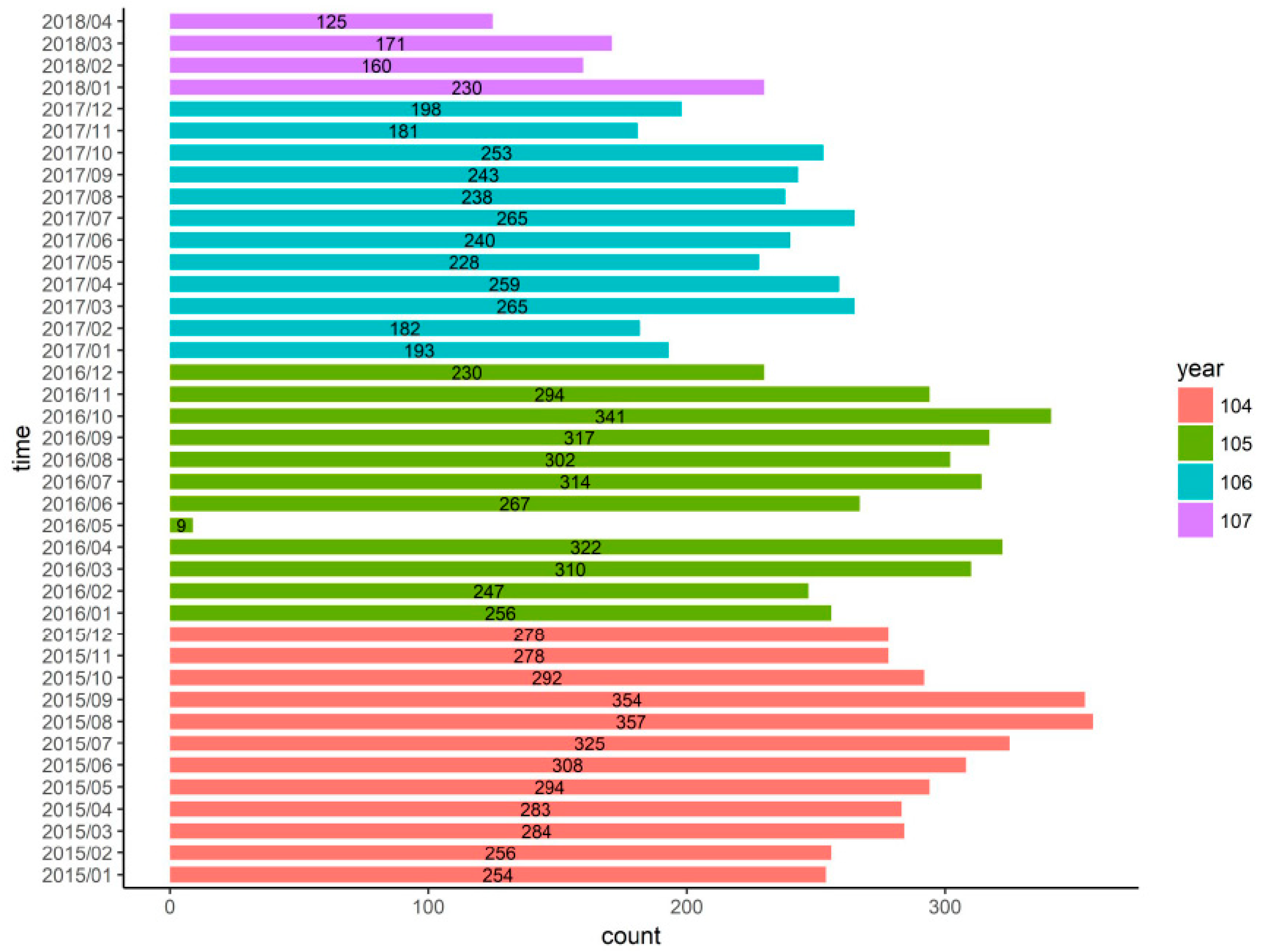
Vehicle Theft data for Taoyuan City was sourced from an open data platform (Open Data Platform of Taiwan: https://data.gov.tw). We chose the Vehicle Theft to be our prediction target because it is obviously affected by environment factors [35]. We used a data period from January 2015 to April 2018, with about 220 criminal incidents occurring each month. The model was used to produce forecasts from January 2017 to April 2018. The collected data were subjected to a simple narrative statistical analysis, with the monthly distributions of reported crimes shown in Figure 1. While the collected open data included some mistakes for May 2016, our experiment used time shift design for validation, thus minimizing the impact of such errors.

We then applied the Google Place API to conduct a landmark radar search of Taoyuan City, using the default support settings to eliminate search results unrelated to Taoyuan City, and produce 84 types of geographic data. Experiments were run using the R language for analysis, while DNN is constructed using the H₂O.ai release package, and the experimental coding and data were placed in GitHub (Project code in GitHub: https://goo.gl/VTWUsY).

3.2. System Workflow

Our system workflow begins with the spatial and temporal. A set of features is then constructed to simulate the crime environment such that these features can be utilized by machine-learning algorithms for crime prediction.

Table 1. Workflow pseudocode.

Workflow Pseudocode

#data preprocessing 1  Create grids from the map’s limited latitude and longitude. The number of grids is the square of n. 2  Let the grids intersect to map M and remove the grids not in map o, M = {g1, g2, g3, …, gn-o}. 3  Crimes which occur in the following month are denoted as y. If no crime occurs in the grid, y = 0. Otherwise, y = 1 and is called a hotspot. 4  If the grid’s y equals zero every month it is called an empty grid and should be removed. Thus, M = {g1, g2, g3, …, gn-(o+e)}. 5  Each grid includes features x. Features are sets of spatial-temporal convolutions (ex. recent 3 months, surround grids) and memory (ex. last year), and count of landmarks called geographical features. 6  In conclusion, g = {y, x1, x2, x3, …, xi}. Note that y is crimes that will occur in the following month, assuming some pattern exists that will produce the probability of crimes occurring. #build models 7  Use machine learning algorithms to learn the pattern, and predict crime for the following month for each gird. 8  Evaluate performance.

shows the workflow pseudocode of the proposed method.

3.3. Models Design

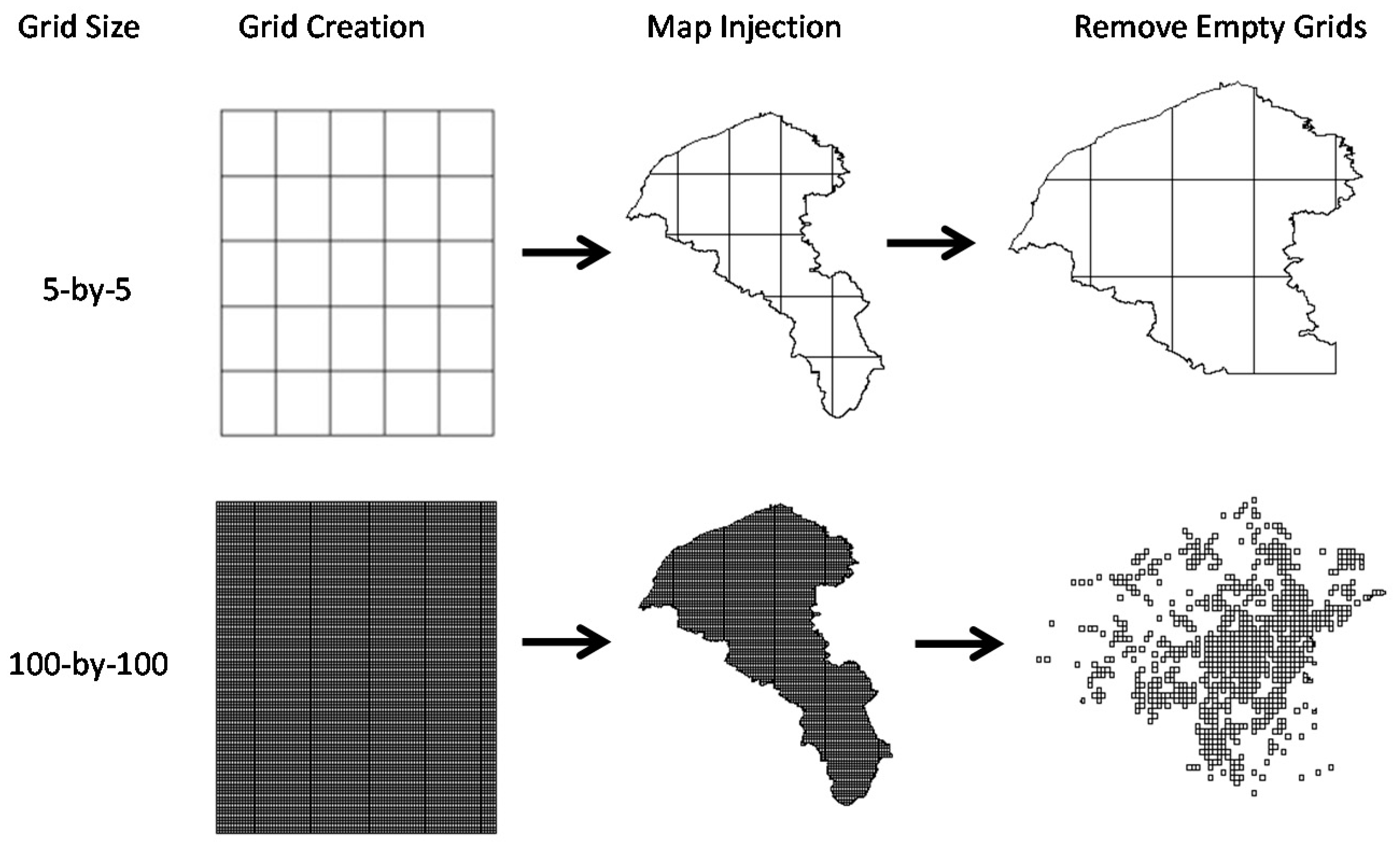
The grid-based space design first defined the borders of Taoyuan City on a map, and then divided the area into 5-by-5 to 100-by-100 grids to produce a grid-based map of the city. We then calculated car and motorcycle thefts for each grid. To optimize the use of computing resources and prevent category imbalance, we then eliminated crime-free grids [17], which typically were located in sparsely-populated suburbs and mountainous areas. This prevents nonoccurring crime categories from exceeding those of crimes which do occur. Specifically, increased grid segmentation will result in increased unbalance, which can lead to the algorithm using the overall learning trend to only predict nonoccurring crimes. While this results in very high accuracy levels, if only nonoccurring crimes are predicted, the model cannot be applied with any meaning; thus, the empty grids must be removed. Sampling techniques can be used to increase categories with low sample numbers, reduce categories with high sample numbers, or produce better virtual samples. However, the application of these methods is no simpler than removing the empty grids, and offers no significant performance advantage. Figure 2 shows the spatial processing flow.

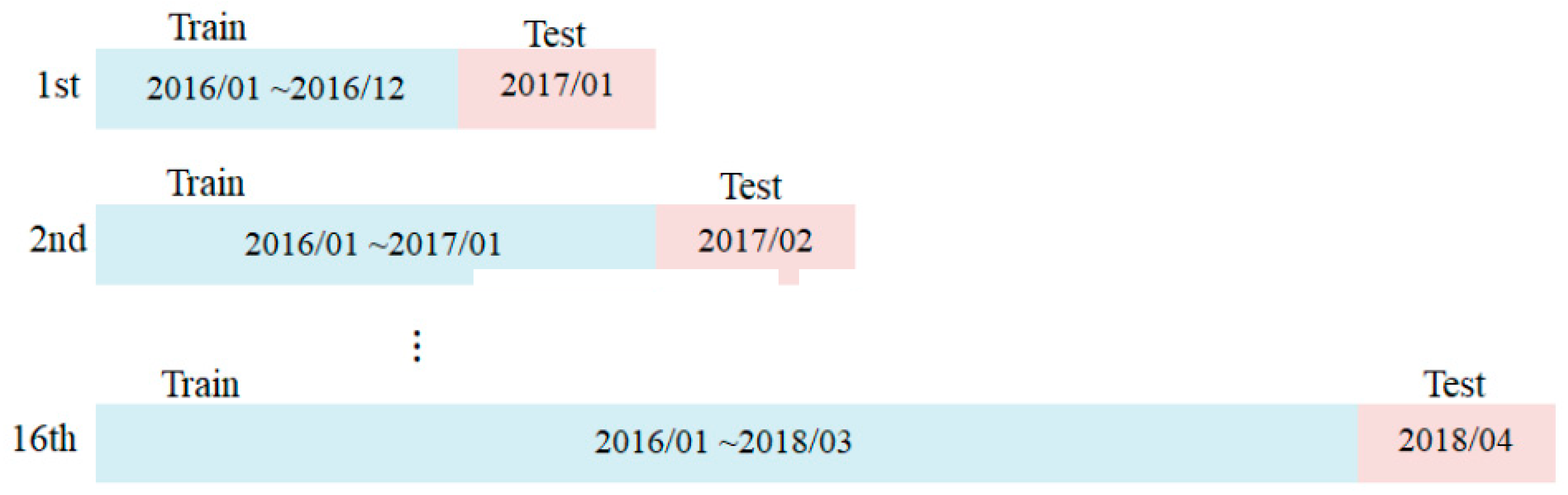
The time design uses individual months as the basic time unit. Supervised learning requires accumulated training samples and lack of sufficient training samples is more likely to produce prediction errors under unknown conditions. Previous experiments have verified that accumulating training samples will enhance model performance [36]. Likewise, the importance of the accumulated data for DNN is discussed in another study [37]. Figure 3 thus shows the time-sliding model design.

3.4. Features Construction

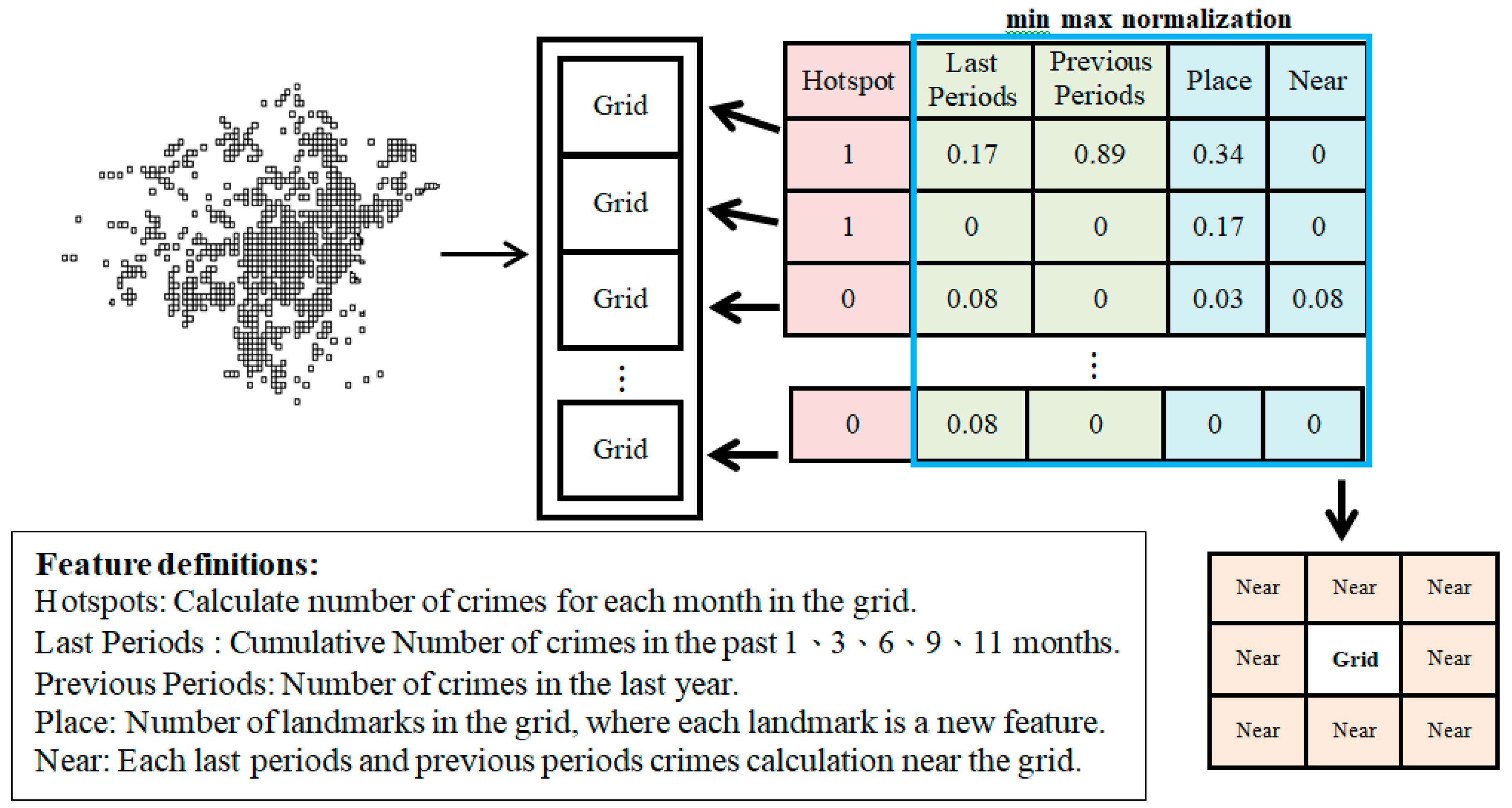
In terms of structural features, we simultaneously consider time and spatial factors, splitting time features into two types: (1) We calculate the accumulated instances of crimes in certain time periods, reflecting the uneven distribution of crime. Broken Windows theory suggests that areas with higher population density or increased presence of gangs or parolees may be correlated with increased crime rates. A current high incidence of crime in an area suggests an increased probability of crime in that area in the near future. (2) Calculating number of crimes committed at the same time in the previous year considers that crimes occur in specific time frames. For example, summer school holidays release large numbers of young people from the constraints of daily school activity, increasing opportunities to form gangs and engage in crime. This design complements the lack of time periodicity considerations in the first feature design.

There are also two kinds of spatial factors, both designed based on a perpetrator’s tendency to commit crimes in a familiar environment: (1) We account for the time and space factors of neighboring grids and make use of the neighborhood characteristics to make predictions [38]. In other words, given the diffuse nature of crime, there is a high likelihood that police activity in one crime-ridden area will push criminals into neighboring areas. (2) In the proposed novel method, we use the Google Place API to generate geographic information queries to simulate the unique environment of each grid area. This considers displacement of criminals [39,40,41] in response to increased localized police activity, assuming that criminals who do shift locations will likely move to areas adjacent to their original location and will follow main roads to the next township. Therefore, the use of geographical features to simulate similar areas can compensate for lack of information in adjacent areas. Figure 4 illustrates the feature calculation and framework.

Finally, a large disparity may occur between features in the same grid, or between different grids with the same feature. To avoid learning being dominated by features with large numbers, we use feature scaling to unify units of measurement for each feature. In this study, min max normalization is used to convert features into values between 0 and 1.

3.5. Baseline

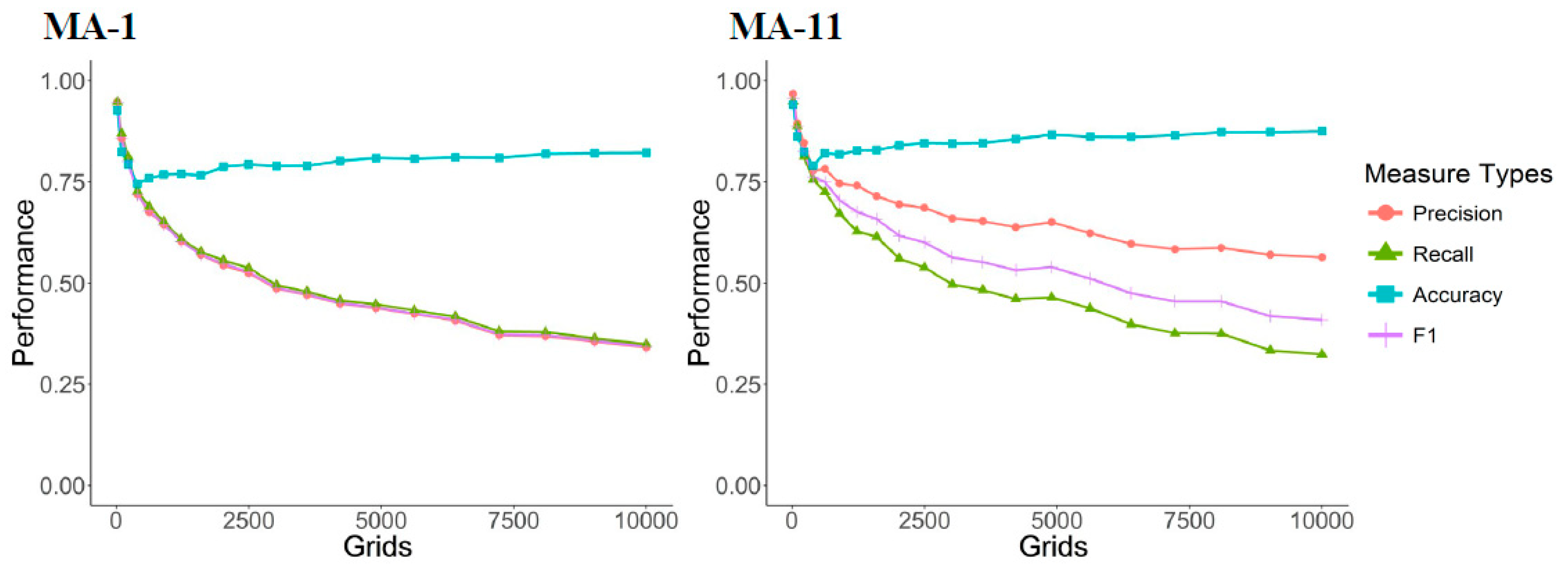
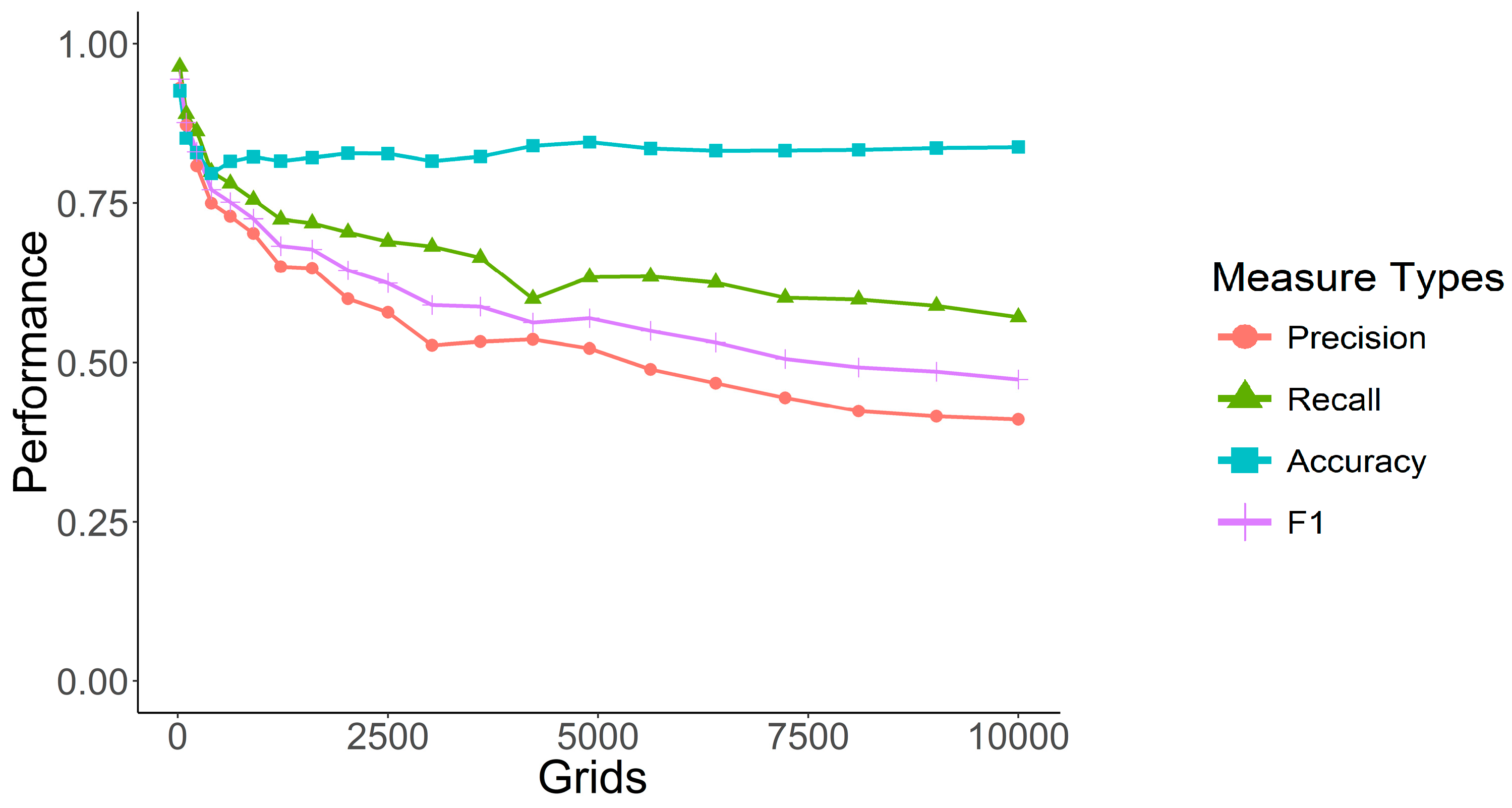
Verifying the performance of the proposed model requires a comparable baseline. Different data sets and design approaches lead to different baselines. This paper uses time series analysis to design the baseline. The most primitive method for time series analysis uses the results from the previous month to predict the subsequent month; however, the results are typically unsatisfactory, and a Moving Average (MA) is used to improve results, with prediction performance shown in Figure 5. Car and motorcycle theft is subject to time and space characteristics. Inputted in the grid, we use the moving average to identify the grid with highest theft incidence. For example, the moving average of the previous 11 months is used to predict the 12th month. If more than half the grid-months show criminal activity, we can predict that grid will also have criminal activity in the 12th month. Precision increases with the MA time interval, but recall will fall; as hot spot prediction accuracy increases, the absolute number of hot spots found falls and will be concentrated in the grids with the highest incidence of crime.

In addition, Figure 5 explains issues related to grid size selection problems. Prediction performance increases with grid size. However, while the largest grid takes the entire city as a single grid, this provides no meaningful prediction. For police purposes, smaller grid sizes are more useful in terms of narrowing the area of interest. However, if the grid size is too small, the likelihood of a crime occurring in a specific place is very low: with a cumulative number in grid close to 0, the data matrix is too sparse to contribute to useful forecasting, thus suitable grid size selection is a critical issue. This study seeks to minimize grid size while meeting specified model performance standards. The baseline is a 100-by-100 grid, which can maintain an F1 score of about 0.4. The F1 standard is used as the performance criterion mainly due to the category imbalance mentioned above. Accuracy will still be high even if the model predicts large numbers of crimes that will not occur. Therefore, it is more appropriate to use the F1 score to reconcile precision and recall. The lower bound of projected performance uses the 11-month MA’s F1 score as a baseline.

3.6. Machine Learning Algorithms

In designing experiments for the crime prediction model, we use DNN-tuning as the main algorithms to compare crime hotspot forecasting performance against other algorithms, including K-Nearest Neighbor (KNN), Support Vector Machine (SVM), and Random Decision Forest (RF).

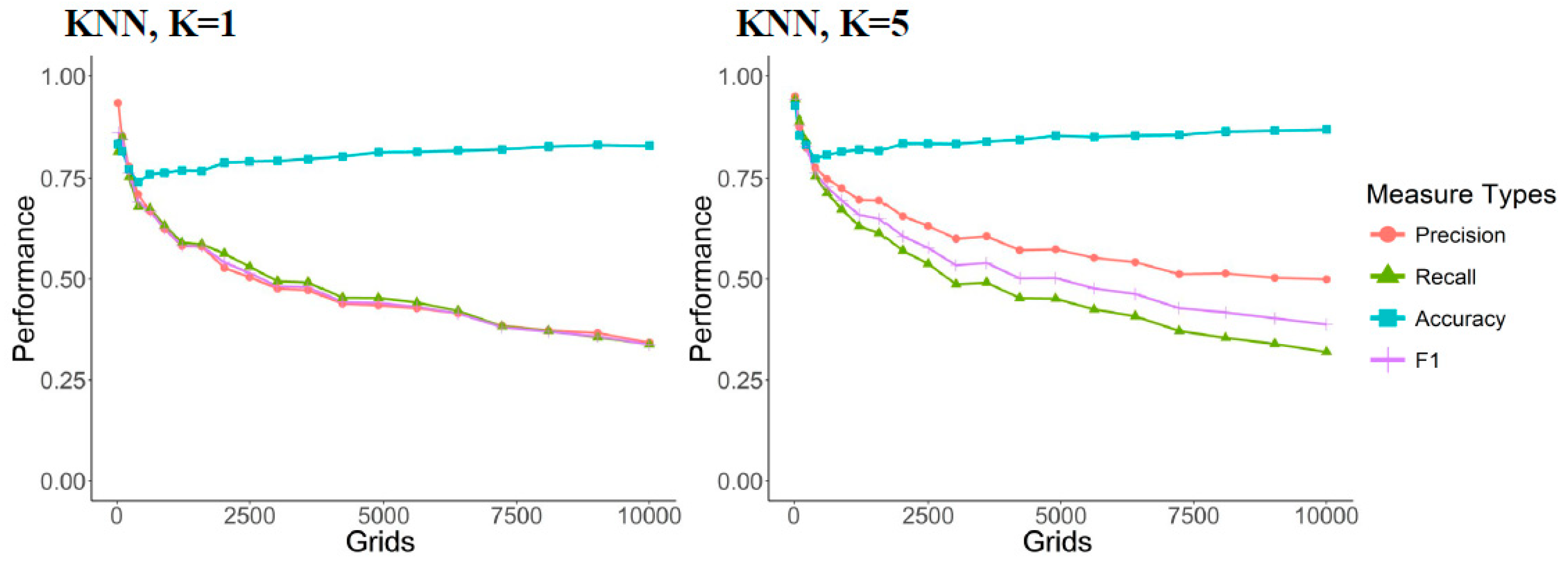
The selection of the KNN algorithm for k is similar to that for MA for the number of months. As shown in Figure 6, as k increases, it gives greater consideration to the nearest neighbors. Through voting, it gradually converges on the most frequently appearing hotspots, thus precision increases while recall decreases, slightly increasing the F1 score. Here we select k = 5 as the control.

Both the SVM and RF algorithms are widely used for classification. SVM uses different types of points to map to high-dimensional space to construct hyperplane separations, mainly to remedy low-dimensional linear inseparability issues and achieve good performance with feature selection [42,43,44]. RF is a classical ensemble algorithm that constructs a random tree by sampling data and features. Finally, random tree predictions are aggregated through voting. Such a structure can reduce the impact of unimportant features, and is well suited to processing unbalanced data sets [45,46].

In DNN-tuning, to prevent overfitting following DNN learning through deeper hidden layers, we use the dropout mechanism [47,48], which has been shown to improve model robustness [49]. We set the dropout to 0.2, i.e., 20% of nodes are randomly discarded at each layer. Each hidden layer is set to 100 neurons, with a total of 9 layers, and uses ReLu as the activation function. Experiments showed ReLu to generally outperform sigmoid [50], and we achieve optimal search results with a learning rate of 0.001, and epochs set to 45. These parameter settings provide some performance improvement.

4. Experiments

4.1. Performance Comparison

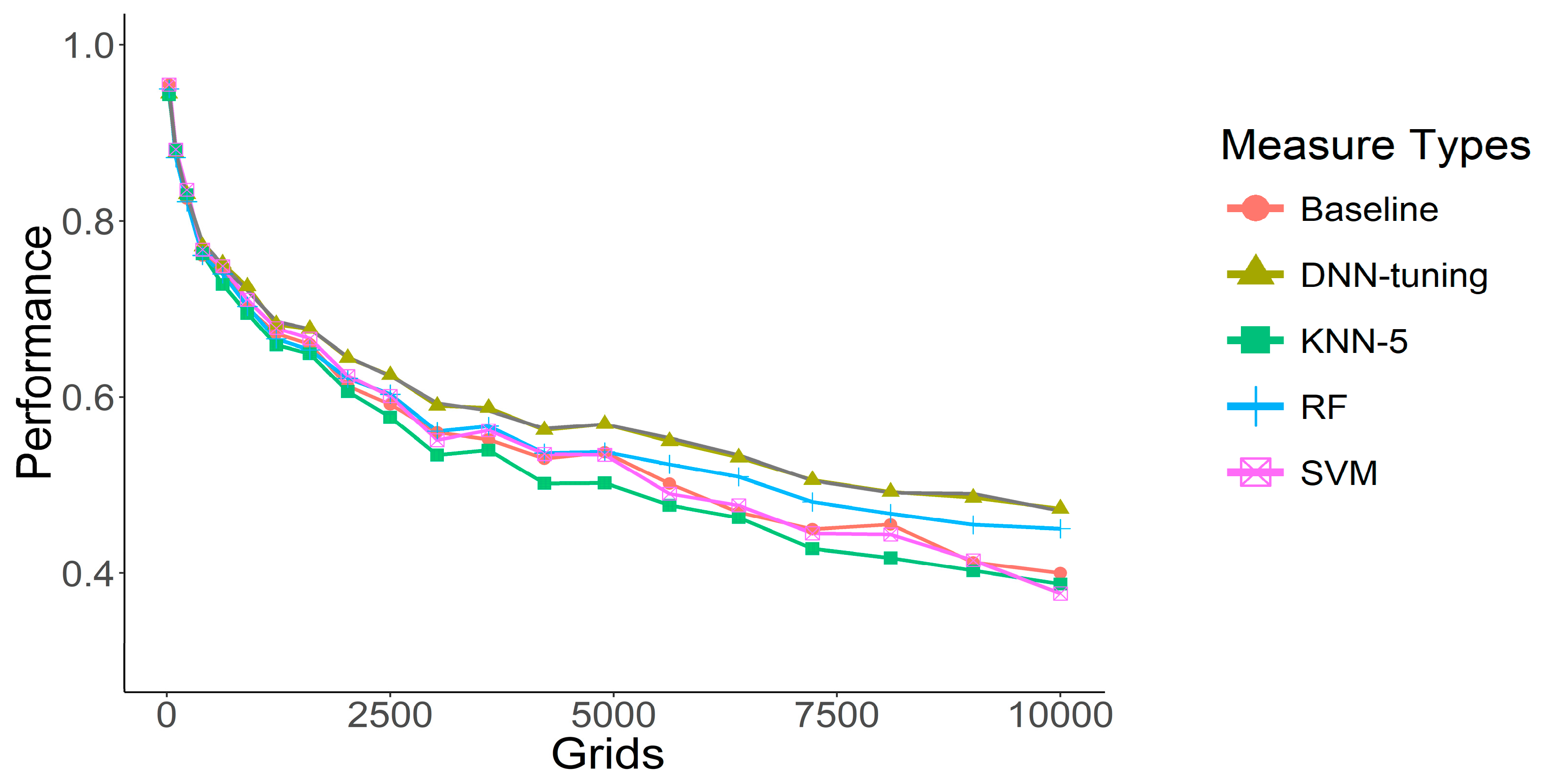
Figure 7 compares the performance of the various algorithms. A t-test was used to determine whether the performance difference among these methods was statistically significant. DNN-tuning provides the best performance for different grid sizes. As shown in

Table 2. Models’ average performance (100-by-100).

Algorithms	F1 Score	Accuracy	Precision	Recall
DNN-tuning	0.4734 *	0.8376	0.4107	0.5708
RF	0.4503 *	0.8197	0.3727	0.5768
baseline	0.4000	0.8784	0.5533	0.3162
SVM	0.3770	0.8810	0.5844	0.2802
KNN, k = 5	0.3877	0.8706	0.4994	0.3194

* DNN-tuning, RF vs. baseline significantly different.

, a 100-by-100 grid produces an F1 score of 0.4734. RF is ranked 2nd, and both algorithms outperform the baseline. The predictive performance of KNN and SVM is lower than the baseline, which can be inferred to be related to the proposed feature design. Both CNN and RF allow for feature adjustment, while KNN and SVM do not. Because this study does not perform feature selection, KNN and SVM underperform the baseline. The detailed performance of DNN-tuning is shown in

Table 3. DNN-tuning performance (100-by-100).

Time	F1 Score	Accuracy	Precision	Recall
2017/01	0.4383	0.8149	0.3308	0.6493
2017/02	0.4326	0.8324	0.3598	0.5423
2017/03	0.5089	0.8398	0.4608	0.5682
2017/04	0.4965	0.8216	0.4109	0.6272
2017/05	0.4411	0.8149	0.3534	0.5867
2017/06	0.5305	0.8531	0.4902	0.5780
2017/07	0.5343	0.8365	0.4768	0.6075
2017/08	0.5355	0.8589	0.5185	0.5537
2017/09	0.4667	0.8274	0.4272	0.5141
2017/10	0.5248	0.8407	0.5146	0.5354
2017/11	0.4644	0.8315	0.3713	0.6197
2017/12	0.4260	0.8390	0.3789	0.4865
2018/01	0.4674	0.8373	0.4322	0.5089
2018/02	0.4146	0.8407	0.3269	0.5667
2018/03	0.4500	0.8539	0.3789	0.5538
2018/04	0.4430	0.8581	0.3400	0.6355
Average	0.4734	0.8376	0.4107	0.5708

.

As shown in Figure 8, DNN-tuning provides optimal predictive performance, showing opposite effects from the baseline and KNN models. It provides better recall performance, but lower precision while still providing a better F1 score than the other models. Note that higher recall is useful to law enforcement for improved crime prediction, thus supporting the main crime prevention strategies despite the lower precision. This allows predeployment of police to prevent crime from occurring, thus recall should be prioritized over precision.

4.2. Variable Importance

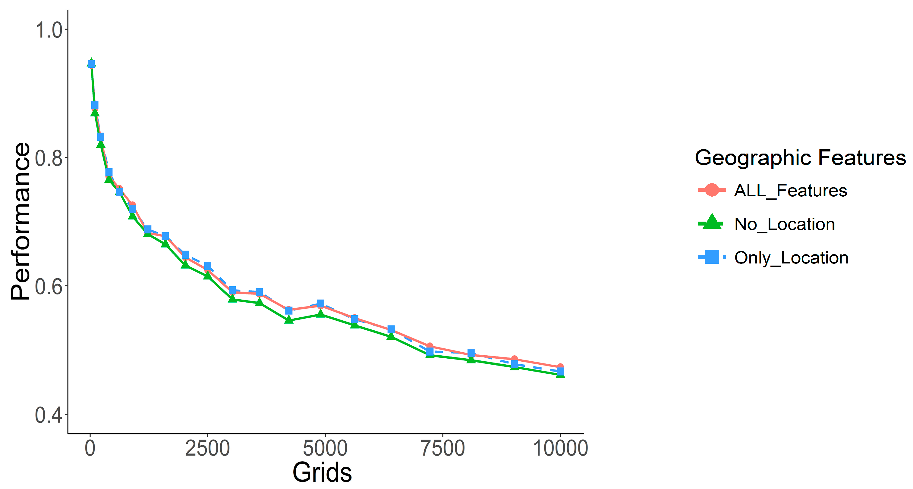
To observe the impact of geographical features on the model, we compared the F1 score performance with different feature designs using DNN-tuning. Figure 9 shows optimal performance for each feature design without considering the lowest performance for geographical features. ALL_Features denotes the prediction model with all design features, No_Location denotes the exclusion of the geographical features, and Only_Location denotes using the geographical features alone. The results of the model that only uses geographic features are little different from that using all features, indicating the high contribution of geographic features for model design in this experiment.

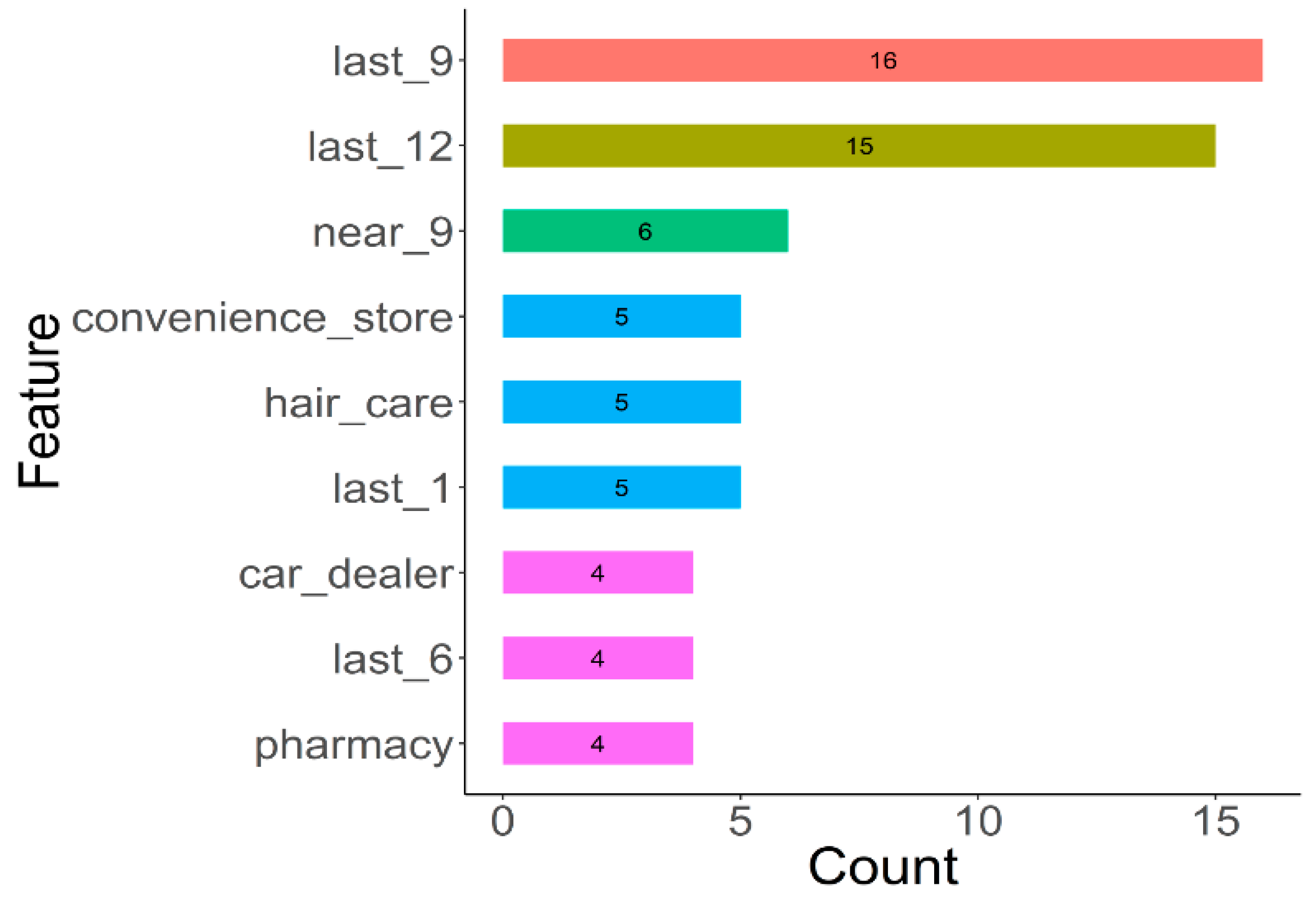
We then eliminate the importance of features in DNN-tuning, calculating the cumulative sum of the 10 most important features of a 16-month period. Figure 10 shows that the time space factors are still the most influential in the grid: over the previous 9 months and previous 12 months. In addition, the surrounding grids also contribute to the DNN-tuning model, while other important features are all geographic features, including convenience stores, hair salons, car dealerships, and pharmacies, all of which are important landmarks given to heavy pedestrian traffic. Note that, in grid-based research, it is very difficult to obtain correct higher-order features for each grid, such as economic level. Data taken from open data or other sources will encounter data granularity problems. Lacking sufficiently detailed information, constructing a grid for each feature is typically accomplished by splitting the average, but this feature does little to distinguish between different grids. However, feature extraction can provide higher-level features [51,52]. Therefore, combining DNN with geographic features better allows us to solve problems for which low-level features are difficult to obtain.

4.3. Detection Crime Displacement

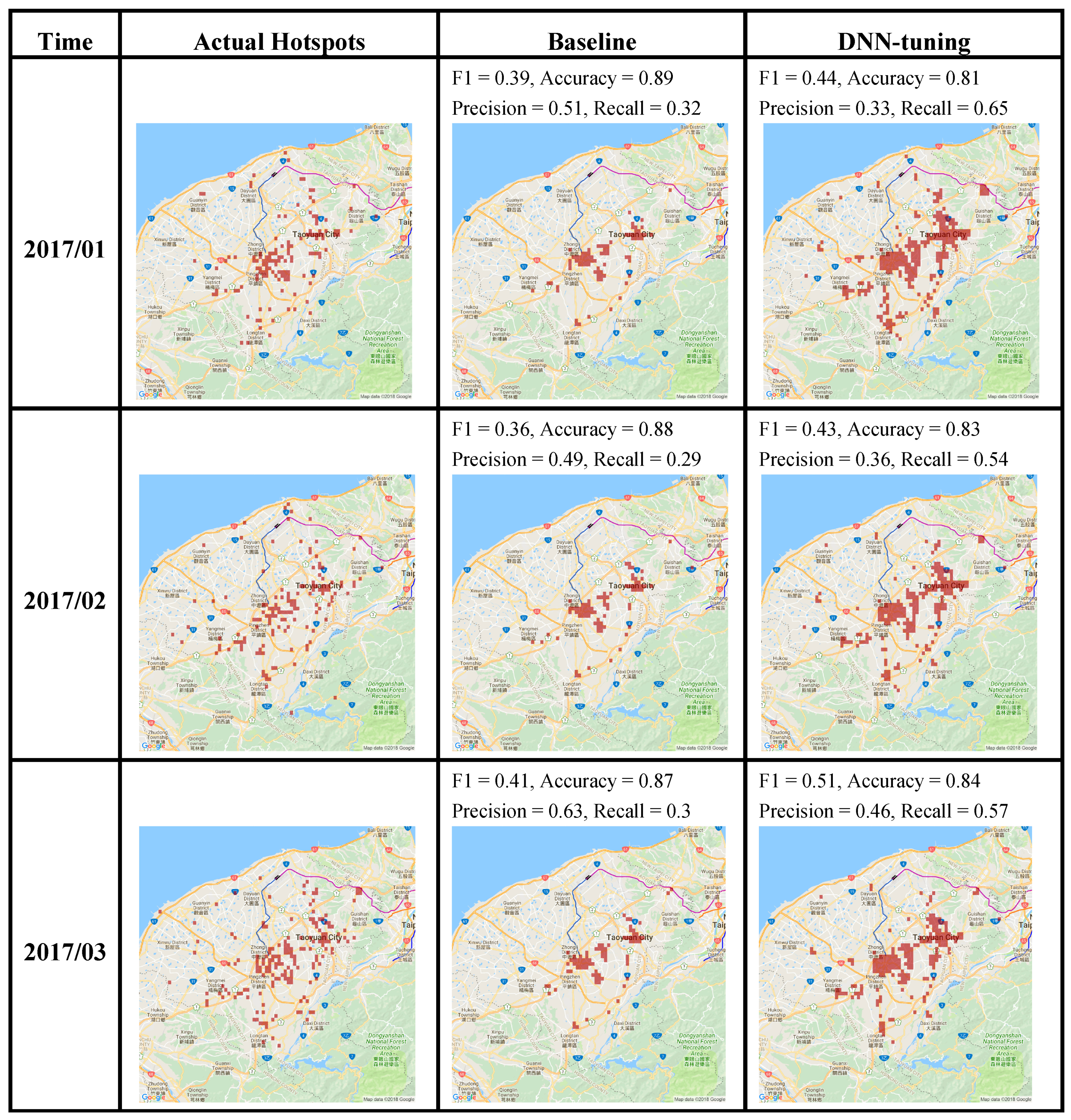
As shown in Figure 11, we visualized the actual hotspots, the baseline, and the optimal model results on Google Maps to determine if the forecasts provided any insight beyond performance improvement. From the baseline, we see little change over three months because, as previously mentioned, the MA will converge on the location with the highest incidence of crime. Because the optimal DNN-tuning model incorporates geographical features for algorithm learning, the model is able to search similar locations for crime hotspots, most of which are along major roads or in urban areas, which is consistent with our assumptions and our understanding of crime displacement.

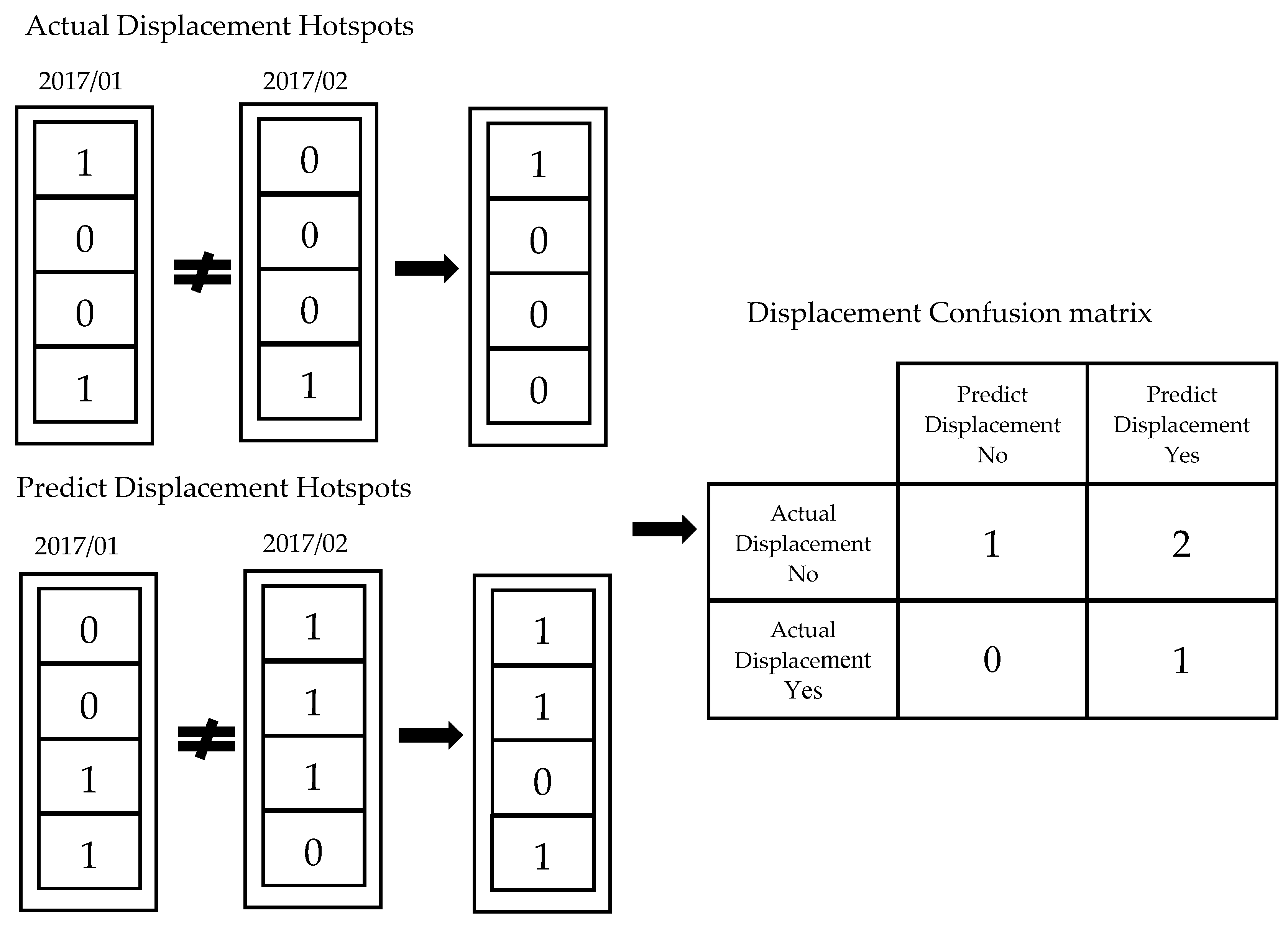
However, the map visualization does not provide a clear representation of the model’s forecast for crime displacement. We thus redesign the displacement prediction scenarios. Figure 12 compares hotspots for two consecutive months, respectively showing displacement and nondisplacement. The actual hotspot displacement and that predicted by the model are recombined in a confusion matrix, where True Positive shows consistency between predicted and actual displacements, and True Negative shows consistency between predicted and actual non-displacement. Thus, precision reflects the model hit rate for crime displacement, and recall reflects the actual rate of crime displacement. These two measures should ideally be improved, thus we use F1 score as a performance measure for the model’s transfer. The results in

Table 4. Displacement performance (100-by-100).

Time	Baseline				DNN-Tuning
	Precision	Recall	Accuracy	F1 Score	Precision	Recall	Accuracy	F1 Score
2017/02	0.6667	0.0625	0.8455	0.1143	0.1719	0.0573	0.8056	0.0859
2017/03	0.4444	0.0396	0.8306	0.0727	0.5135	0.0941	0.8331	0.1590
2017/04	0.4167	0.0228	0.8164	0.0433	0.5147	0.1598	0.8198	0.2439
2017/05	0.4706	0.0379	0.8239	0.0702	0.2743	0.1469	0.7824	0.1914
2017/06	0.3750	0.0141	0.8214	0.0271	0.3636	0.1315	0.8056	0.1931
2017/07	0.5625	0.0419	0.8231	0.0779	0.3125	0.0698	0.8065	0.1141
2017/08	0.4167	0.0230	0.8181	0.0437	0.3421	0.0599	0.8098	0.1020
2017/09	0.4286	0.0261	0.8073	0.0492	0.4390	0.1565	0.8007	0.2308
2017/10	0.5385	0.0304	0.8098	0.0576	0.2414	0.0609	0.7841	0.0972
2017/11	0.6667	0.0441	0.8156	0.0826	0.3636	0.0529	0.8040	0.0923
2017/12	0.4000	0.0309	0.8364	0.0574	0.5357	0.0773	0.8405	0.1351
2018/01	0.5500	0.0480	0.8115	0.0884	0.4762	0.0437	0.8090	0.0800
2018/02	0.8182	0.0448	0.8389	0.0849	0.3846	0.0746	0.8256	0.1250
2018/03	0.5000	0.0479	0.8439	0.0874	0.2273	0.0532	0.8239	0.0862
2018/04	0.5000	0.0537	0.8762	0.0970	0.3235	0.0738	0.8663	0.1202
Average:	0.5170	0.0378	0.8279	0.0702	0.3656	0.0875	0.8145	0.1371 *

* DNN-tuning vs. baseline significantly different.

show that DNN-tuning outperforms the baseline prediction for most months.

5. Conclusions

The time and spatial characteristics allow machine learning to be applied to crime prediction. Traditional crime prevention strategies also use time and spatial factors, but these methods rely heavily on the personal experience of senior law enforcement officers, and the storage, transfer, and application of this experience are difficult to automate. Therefore, the present study attempts to collect and model such experience, integrating geographic features and machine-learning techniques to improve model prediction performance and provide police with a useful reference for forecasting crime. The proposed model has an advantage in that it provides a more objective basis for comparison, and allows for the replication, transmission, and continuous improvement of the knowledge model.

The main contribution of the present study is to use more recent machine-learning techniques, including the concept of feature learning, along with dropout and tuning methods. Applied to traditional grid-based approaches, these methods show that an excessively small feature training set results in excessive information overlap, thus making it difficult to distinguish different vector spaces. Insufficient data will lead to inaccurate measurements in unknown conditions. Therefore, we can use features and data volume to improve the upper bound of prediction performance, but large numbers of features may reduce prediction accuracy due to weak correlations. This is why DNN outperforms traditional machine-learning techniques and time-series approaches, providing a breakthrough in feature learning and allowing us to use more, and more complicated, features to enhance data differentiation, without being influenced by the weak correlations of excessive features, and thus improving prediction performance. However, we do not propose increasing an excessive number of features indefinitely, which would result in the curse of dimensionality. In addition to producing an excessively sparse data matrix, this will greatly increase computational time and resource requirements, as all the features would need to be processed. In terms of time efficiency, the proposed DNN-tuning requires 27 min on average for training on a PC with an Intel Xeon 2.1 GHz CPU, and 32 GB memory. Although the proposed deep learning method is more complex than traditional methods, it can yield performance improvements of 2–7%.

The second contribution is to explain the difficulty in obtaining high-level features in the grid, but that this can be simplified by obtaining landmarks in Google Place, allowing us to calculate landmark features in the grid to establish geographic features that, combined with feature learning, may be used to extract higher-level features and thus improve model efficiency. The other advantage of geographic features is that they may be used to simulate and predict crime displacement. When planning overall crime prevention strategies, police can leverage knowledge of current high-risk crime grids to forecast future high-risk areas.

Finally, even considering that powerful technology tools must still combine the experience of law enforcement officers with criminological theory, attempting to further model police expertise and the use of police databases is likely to enhance the model’s predictive power. Geographic features can include crime-related locations, including bars, KTVs, and gang territories, along with crime-inhibiting features such as streetlights, CCTV cameras, police stations, and neighborhood watch. Environmental features include weather and temperature, or physical characteristics such as Natural Surveillance [53]. In addition, displacement features like police actions, controls, and buffer zones can be considered to simulate displacement effects more precisely [54].

We hope the results of this study can be used to improve grid-based crime prediction models and encourage discussion on the integrating accumulation and feature design of data for characterization learning, and promote the modeling of law enforcement experience and criminology theory.

References

- Short, M.B.; D’orsogna, M.R.; Pasour, V.B.; Tita, G.E.; Brantingham, P.J.; Bertozzi, A.L.; Chayes, L.B. A statistical model of criminal behavior. Math. Models Methods Appl. Sci. 2008, 18, 1249–1267. [Google Scholar] [CrossRef]
- Tayebi, M.A.; Glässer, U. Personalized crime location prediction. In Social Network Analysis in Predictive Policing; Springer: Cham, Switzerland, 2016; pp. 99–126. [Google Scholar]
- Leong, K.; Sung, A. A review of spatio-temporal pattern analysis approaches on crime analysis. Int. E J. Crim. Sci. 2015, 9, 1–33. [Google Scholar]
- Perry, W.L. Predictive Policing: The Role of Crime Forecasting in Law Enforcement Operations; Rand Corporation: Santa Monica, CA, USA, 2013. [Google Scholar]
- Wang, X.; Brown, D.E. The spatio-temporal modeling for criminal incidents. Secur. Inform. 2012, 1, 2. [Google Scholar] [CrossRef] [Green Version]
- Kajita, M.; Kajita, S. Crime Prediction by Data-Driven Green’s Function method. arXiv, 2017; arXiv:1704.00240. [Google Scholar]
- Almanie, T.; Mirza, R.; Lor, E. Crime prediction based on crime types and using spatial and temporal criminal hotspots. arXiv, 2015; arXiv:1508.02050. [Google Scholar] [CrossRef]
- Wang, D.; Ding, W.; Lo, H.; Stepinski, T.; Salazar, J.; Morabito, M. Crime hotspot mapping using the crime related factors—A spatial data mining approach. Appl. Intell. 2013, 39, 772–781. [Google Scholar] [CrossRef]
- Wang, X.; Gerber, M.S.; Brown, D.E. Automatic crime prediction using events extracted from twitter posts. In Proceedings of the International Conference on Social Computing, Behavioral-Cultural Modeling, and Prediction, College Park, MD, USA, 3–5 April 2012; Springer: Berlin/Heidelberg, Germany, 2012; pp. 231–238. [Google Scholar]
- Gerber, M.S. Predicting crime using Twitter and kernel density estimation. Decis. Support Syst. 2014, 61, 115–125. [Google Scholar] [CrossRef]
- Yang, J.; Eickhoff, C. Unsupervised Spatio-Temporal Embeddings for User and Location Modelling. arXiv, 2017; arXiv:1704.03507. [Google Scholar]
- Zhao, X.; Tang, J. Modeling Temporal-Spatial Correlations for Crime Prediction. In Proceedings of the 2017 ACM on Conference on Information and Knowledge Management, Singapore, 6–10 November 2017; pp. 497–506. [Google Scholar]
- Sypion-Dutkowska, N.; Leitner, M. Land use influencing the spatial distribution of urban crime: A case study of Szczecin, Poland. ISPRS Int. J. Geo-Inf. 2017, 6, 74. [Google Scholar] [CrossRef]
- Yue, H.; Zhu, X.; Ye, X.; Guo, W. The Local Colocation Patterns of Crime and Land-Use Features in Wuhan, China. ISPRS Int. J. Geo-Inf. 2017, 6, 307. [Google Scholar] [CrossRef]
- Liu, H.; Zhu, X. Joint Modeling of Multiple Crimes: A Bayesian Spatial Approach. ISPRS Int. J. Geo-Inf. 2017, 6, 16. [Google Scholar] [CrossRef]
- Duan, L.; Ye, X.; Hu, T.; Zhu, X. Prediction of Suspect Location Based on Spatiotemporal Semantics. ISPRS Int. J. Geo-Inf. 2017, 6, 185. [Google Scholar] [CrossRef]
- Yu, C.H.; Ward, M.W.; Morabito, M.; Ding, W. Crime forecasting using data mining techniques. In Proceedings of the 2011 IEEE 11th International Conference on Data Mining Workshops (ICDMW), Vancouver, BC, Canada, 11 December 2011; pp. 779–786. [Google Scholar]
- Wang, B.; Yin, P.; Bertozzi, A.L.; Brantingham, P.J.; Osher, S.J.; Xin, J. Deep Learning for Real-Time Crime Forecasting and its Ternarization. arXiv 2017, arXiv:1711.08833. [Google Scholar]
- Swietojanski, P.; Ghoshal, A.; Renals, S. Unsupervised cross-lingual knowledge transfer in DNN-based LVCSR. In Proceedings of the 2012 IEEE Spoken Language Technology Workshop (SLT), Miami, FL, USA, 2–5 December 2012; pp. 246–251. [Google Scholar]
- Sun, S.; Zhang, B.; Xie, L.; Zhang, Y. An unsupervised deep domain adaptation approach for robust speech recognition. Neurocomputing 2017, 257, 79–87. [Google Scholar] [CrossRef]
- Dahl, G.E.; Yu, D.; Deng, L.; Acero, A. Context-dependent pre-trained deep neural networks for large-vocabulary speech recognition. IEEE Trans. Audio Speech Lang. Process. 2012, 20, 30–42. [Google Scholar] [CrossRef]
- Mitra, V.; Sivaraman, G.; Nam, H.; Espy-Wilson, C.; Saltzman, E. Articulatory features from deep neural networks and their role in speech recognition. In Proceedings of the 2014 IEEE International Conference on Acoustics, Speech and Signal Processing (ICASSP), Florence, Italy, 4–9 May 2014; pp. 3017–3021. [Google Scholar]
- Ali, H.; Tran, S.N.; Benetos, E.; Garcez, A.S.D.A. Speaker recognition with hybrid features from a deep belief network. Neural Comput. Appl. 2018, 29, 13–19. [Google Scholar] [CrossRef]
- Wang, S.; Jiang, Y.; Chung, F.L.; Qian, P. Feedforward kernel neural networks, generalized least learning machine, and its deep learning with application to image classification. Appl. Soft Comput. 2015, 37, 125–141. [Google Scholar] [CrossRef]
- Ciregan, D.; Meier, U.; Schmidhuber, J. Multi-column deep neural networks for image classification. In Proceedings of the 2012 IEEE Conference on Computer Vision and Pattern Recognition (CVPR), Singapore, 16–21 June 2012; pp. 3642–3649. [Google Scholar]
- Uzair, M.; Shafait, F.; Ghanem, B.; Mian, A. Representation learning with deep extreme learning machines for efficient image set classification. Neural Comput. Appl. 2015, 30, 1–13. [Google Scholar] [CrossRef]
- Arunkumar, R.; Karthigaikumar, P. Multi-retinal disease classification by reduced deep learning features. Neural Comput. Appl. 2017, 28, 329–334. [Google Scholar] [CrossRef]
- Vilares, D.; Doval, Y.; Alonso, M.A.; Gómez-Rodríguez, C. LyS at SemEval-2016 task 4: Exploiting neural activation values for Twitter sentiment classification and quantification. In Proceedings of the 10th International Workshop on Semantic Evaluation (SemEval), San Diego, CA, USA, 16–17 June 2016; pp. 79–84. [Google Scholar]
- Wang, J.; Yu, L.C.; Lai, K.R.; Zhang, X. Dimensional sentiment analysis using a regional CNN-LSTM model. In Proceedings of the 54th Annual Meeting of the Association for Computational Linguistics (ACL), Berlin, Germany, 7–12 August 2016; pp. 225–230. [Google Scholar]
- Goel, P.; Kulshreshtha, D.; Jain, P.; Shukla, K.K. Prayas at EmoInt 2017: An ensemble of deep neural architectures for emotion intensity prediction in Tweets. In Proceedings of the 8th Workshop on Computational Approaches to Subjectivity, Sentiment and Social Media Analysis (WASSA), Copenhagen, Denmark, 8 September 2017; pp. 58–65. [Google Scholar]
- Yu, L.C.; Wang, J.; Lai, K.R.; Zhang, X. Refining word embeddings using intensity scores for sentiment analysis. IEEE/ACM Trans. Audio Speech Lang. Process. 2018, 26, 671–681. [Google Scholar] [CrossRef]
- Yu, L.C.; Wang, J.; Lai, K.R.; Zhang, X. Pipelined neural networks for phrase-level sentiment intensity prediction. IEEE Trans. Affect. Comput. 2018. [Google Scholar] [CrossRef]
- Putin, E.; Mamoshina, P.; Aliper, A.; Korzinkin, M.; Moskalev, A.; Kolosov, A.; Zhavoronkov, A. Deep biomarkers of human aging: Application of deep neural networks to biomarker development. Aging (Albany NY) 2016, 8, 1021. [Google Scholar] [CrossRef] [PubMed]
- Bengio, Y.; Courville, A.; Vincent, P. Representation learning: A review and new perspectives. IEEE Trans. Pattern Anal. Mach. Intell. 2013, 35, 1798–1828. [Google Scholar] [CrossRef] [PubMed]
- Piza, E.; Feng, S.; Kennedy, L.; Caplan, J. Place-based correlates of motor vehicle theft and recovery: Measuring spatial influence across neighborhood context. Urban Stud. 2017, 54, 2998–3021. [Google Scholar] [CrossRef]
- Lin, Y.L.; Chen, T.Y.; Yu, L.C. Using Machine Learning to Assist Crime Prevention. In Proceedings of the 2017 6th IIAI International Congress on Advanced Applied Informatics (IIAI-AAI), Shizuoka, Japan, 9–13 July 2017; pp. 1029–1030. [Google Scholar]
- Zhang, J.; Zheng, Y.; Qi, D.; Li, R.; Yi, X. DNN-based prediction model for spatio-temporal data. In Proceedings of the 24th ACM SIGSPATIAL International Conference on Advances in Geographic Information Systems, Burlingame, CA, USA, 31 October–3 November 2016; p. 92. [Google Scholar]
- Marco, M.; Gracia, E.; López-Quílez, A. Linking neighborhood characteristics and drug-related police interventions: A Bayesian spatial analysis. ISPRS Int. J. Geo-Inf. 2017, 6, 65. [Google Scholar] [CrossRef]
- Weisburd, D.; Telep, C.W. Hot spots policing: What we know and what we need to know. J. Contemp. Crim. Justice 2014, 30, 200–220. [Google Scholar] [CrossRef]
- Telep, C.W.; Weisburd, D.; Gill, C.E.; Vitter, Z.; Teichman, D. Displacement of crime and diffusion of crime control benefits in large-scale geographic areas: A systematic review. J. Exp. Criminol. 2014, 10, 515–548. [Google Scholar] [CrossRef]
- Ariel, B.; Partridge, H. Predictable policing: Measuring the crime control benefits of hotspots policing at bus stops. J. Quant. Criminol. 2017, 33, 809–833. [Google Scholar] [CrossRef]
- Zhou, X.; Wang, J. Feature selection for image classification based on a new ranking criterion. J. Comput. Commun. 2015, 3, 74. [Google Scholar] [CrossRef]
- Luo, L.; Chen, X. Integrating piecewise linear representation and weighted support vector machine for stock trading signal prediction. Appl. Soft Comput. 2013, 13, 806–816. [Google Scholar] [CrossRef]
- Cervantes, J.; Lamont, F.G.; López-Chau, A.; Mazahua, L.R.; Ruíz, J.S. Data selection based on decision tree for SVM classification on large data sets. Appl. Soft Comput. 2015, 37, 787–798. [Google Scholar] [CrossRef] [Green Version]
- Del Río, S.; López, V.; Benítez, J.M.; Herrera, F. On the use of MapReduce for imbalanced big data using Random Forest. Inf. Sci. 2014, 285, 112–137. [Google Scholar] [CrossRef]
- Li, Y.; Yan, C.; Liu, W.; Li, M. A principle component analysis-based random forest with the potential nearest neighbor method for automobile insurance fraud identification. Appl. Soft Comput. 2017. [Google Scholar] [CrossRef]
- Srivastava, N.; Hinton, G.E.; Krizhevsky, A.; Sutskever, I.; Salakhutdinov, R. Dropout: A simple way to prevent neural networks from overfitting. J. Mach. Learn. Res. 2014, 15, 1929–1958. [Google Scholar]
- Aljundi, R.; Babiloni, F.; Elhoseiny, M.; Rohrbach, M.; Tuytelaars, T. Memory Aware Synapses: Learning what (not) to forget. arXiv, 2017; arXiv:1711.09601. [Google Scholar]
- Lin, M.; Chen, Q.; Yan, S. Network in network. arXiv, 2013; arXiv:1312.4400. [Google Scholar]
- Simpson, A.J. Taming the ReLU with Parallel Dither in a Deep Neural Network. arXiv, 2015; arXiv:1509.05173. [Google Scholar]
- Wang, Y.; Hu, S. Exploiting high level feature for dynamic textures recognition. Neurocomputing 2015, 154, 217–224. [Google Scholar] [CrossRef]
- Wehrmann, J.; Barros, R.C. Movie genre classification: A multi-label approach based on convolutions through time. Appl. Soft Comput. 2017, 61, 973–982. [Google Scholar] [CrossRef]
- Lee, I.; Jung, S.; Lee, J.; Macdonald, E. Street crime prediction model based on the physical characteristics of a streetscape: Analysis of streets in low-rise housing areas in South Korea. Environ. Plan. B Urban Anal. City Sci. 2017. [Google Scholar] [CrossRef]
- Bowers, K.J.; Johnson, S.D. Measuring the geographical displacement and diffusion of benefit effects of crime prevention activity. J. Quant. Criminol. 2003, 19, 275–301. [Google Scholar] [CrossRef]
© 2018 by the authors. Licensee MDPI, Basel, Switzerland. This article is an open access article distributed under the terms and conditions of the Creative Commons Attribution (CC BY) license (http://creativecommons.org/licenses/by/4.0/).