Seamless Upscaling of the Field-Measured Grassland Aboveground Biomass Based on Gaussian Process Regression and Gap-Filled Landsat 8 OLI Reflectance


 and
and 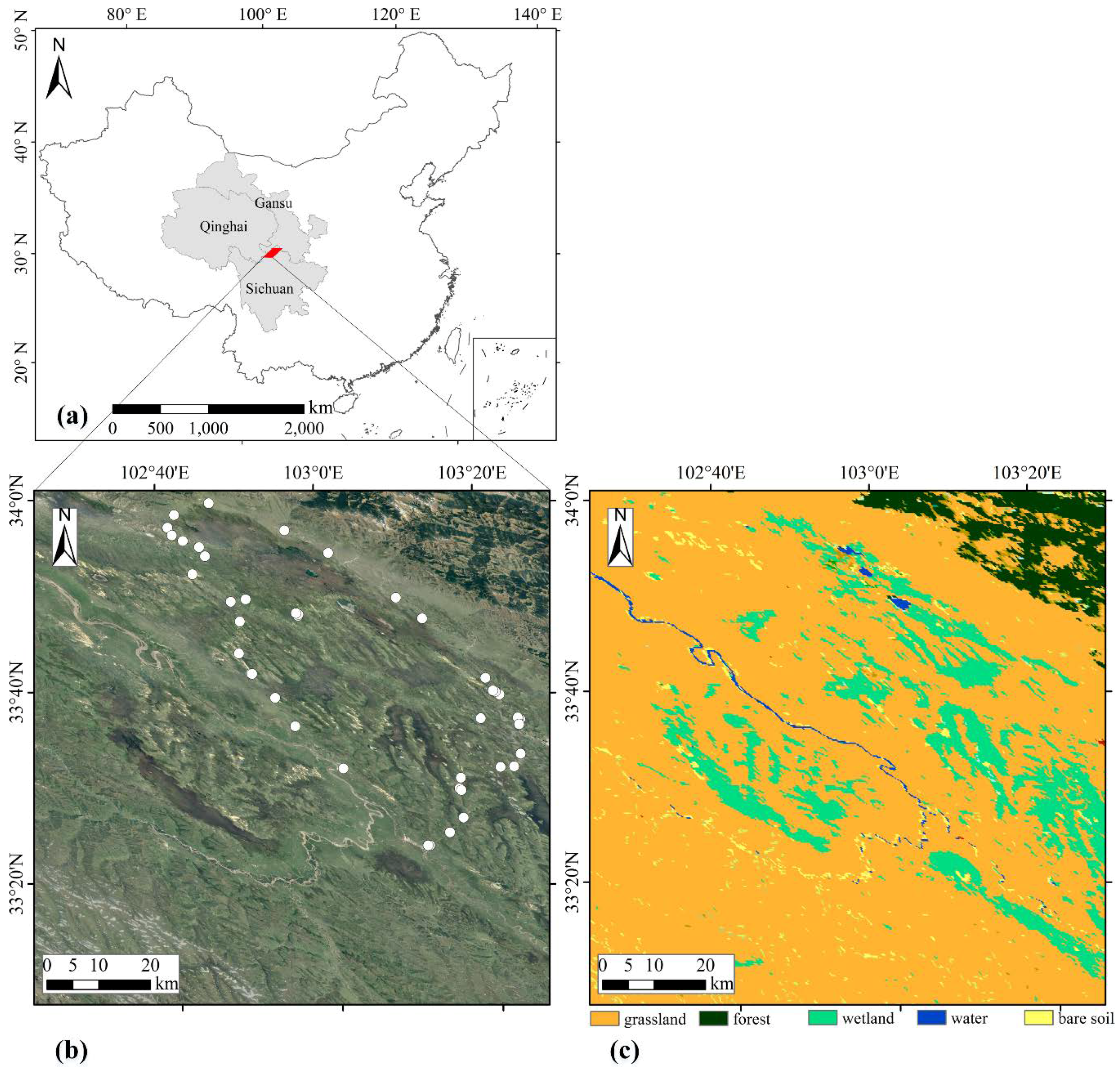
Abstract
1. Introduction
2. Data Collection
2.1. Study Area and Field Measurements
2.2. Landsat 8 OLI Reflectance Data
2.3. MCD43A4 Reflectance Data
3. Methodology
3.1. CACAO Method
3.2. Gaussian Process Regression
3.3. Function Regression between Field Measurements and Vegetation Indices
3.4. Assessment Method
4. Results
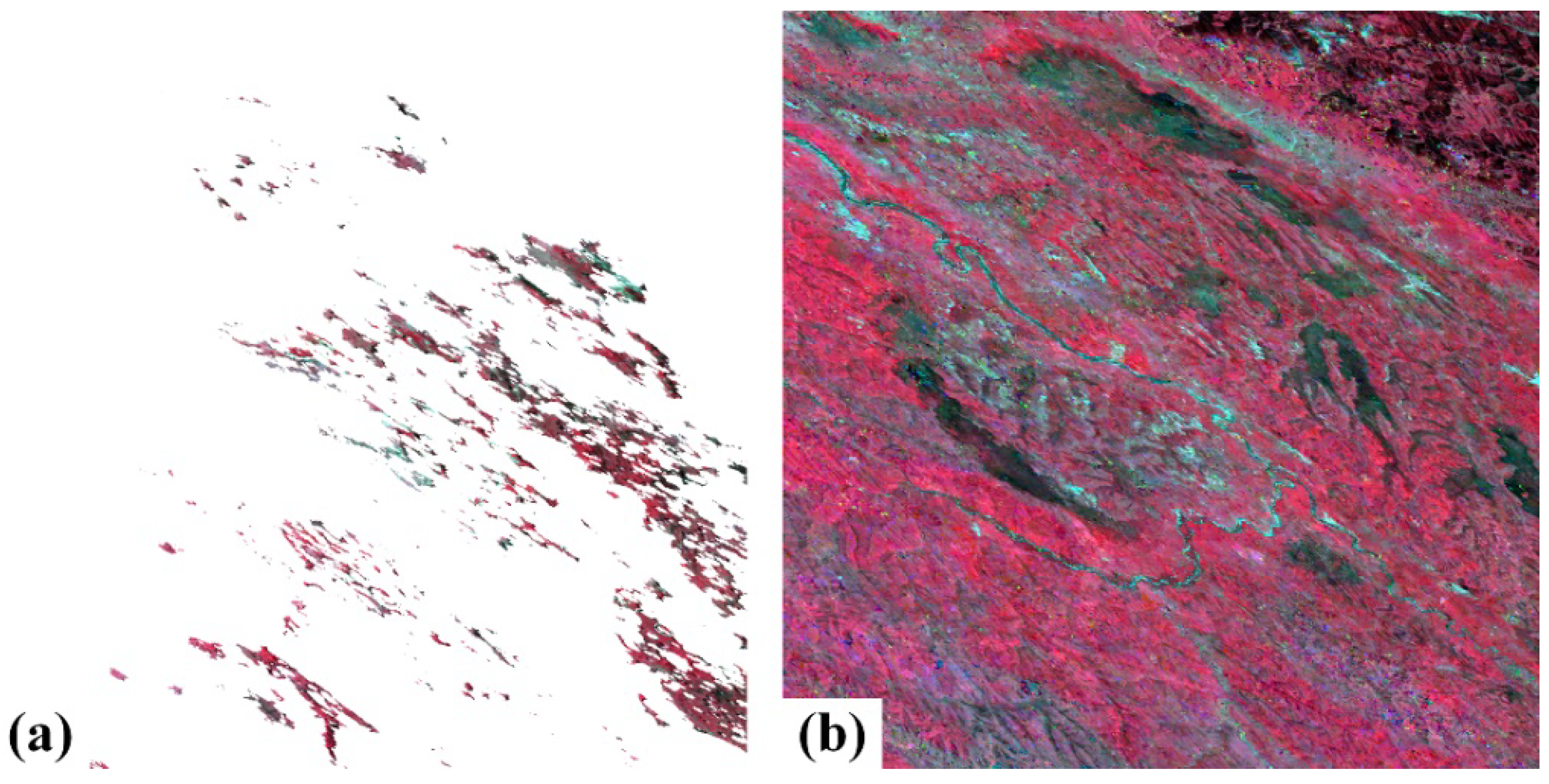
4.1. Gap-Filled Reflectance
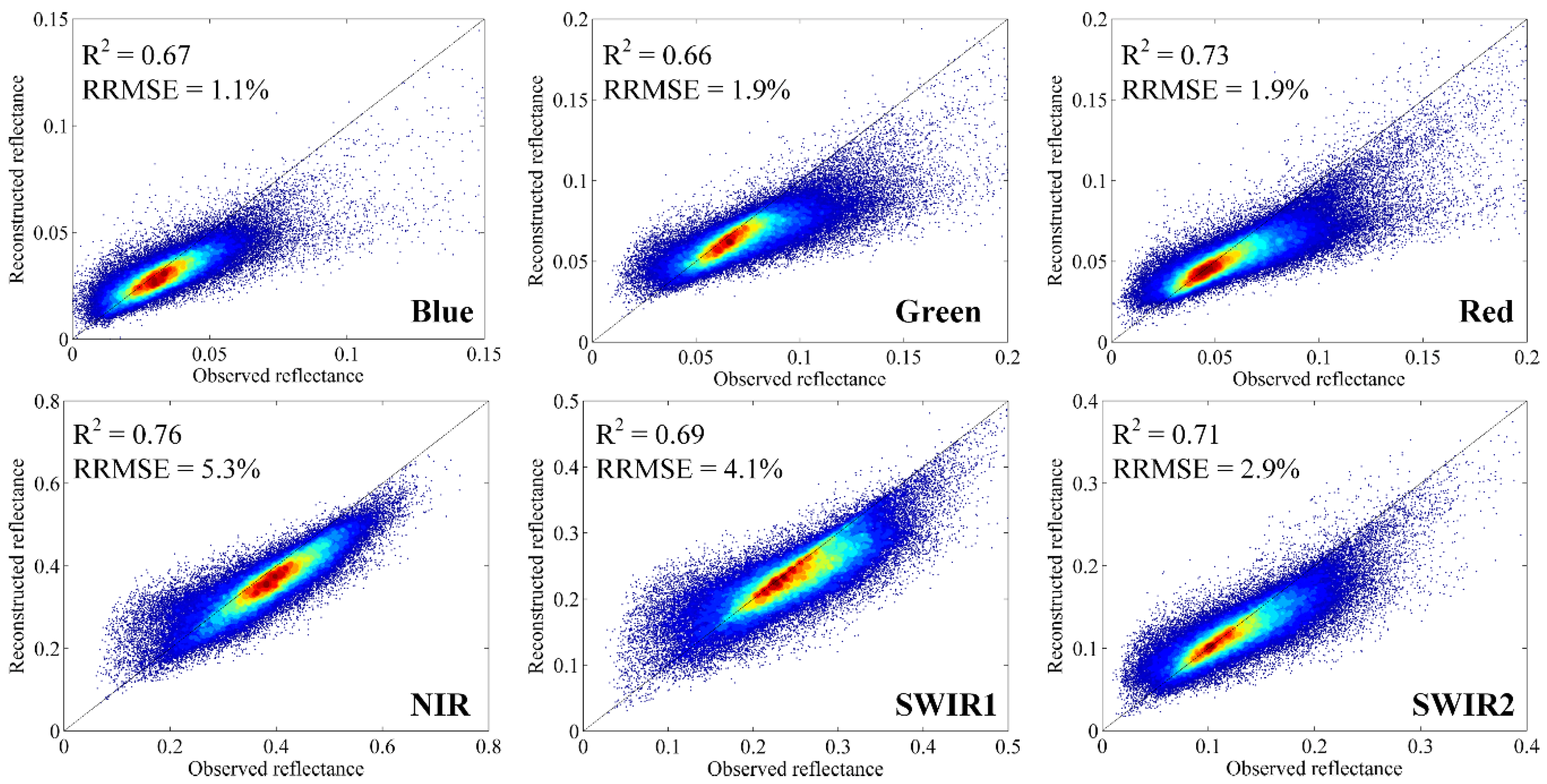
4.2. Upscaling Assessment
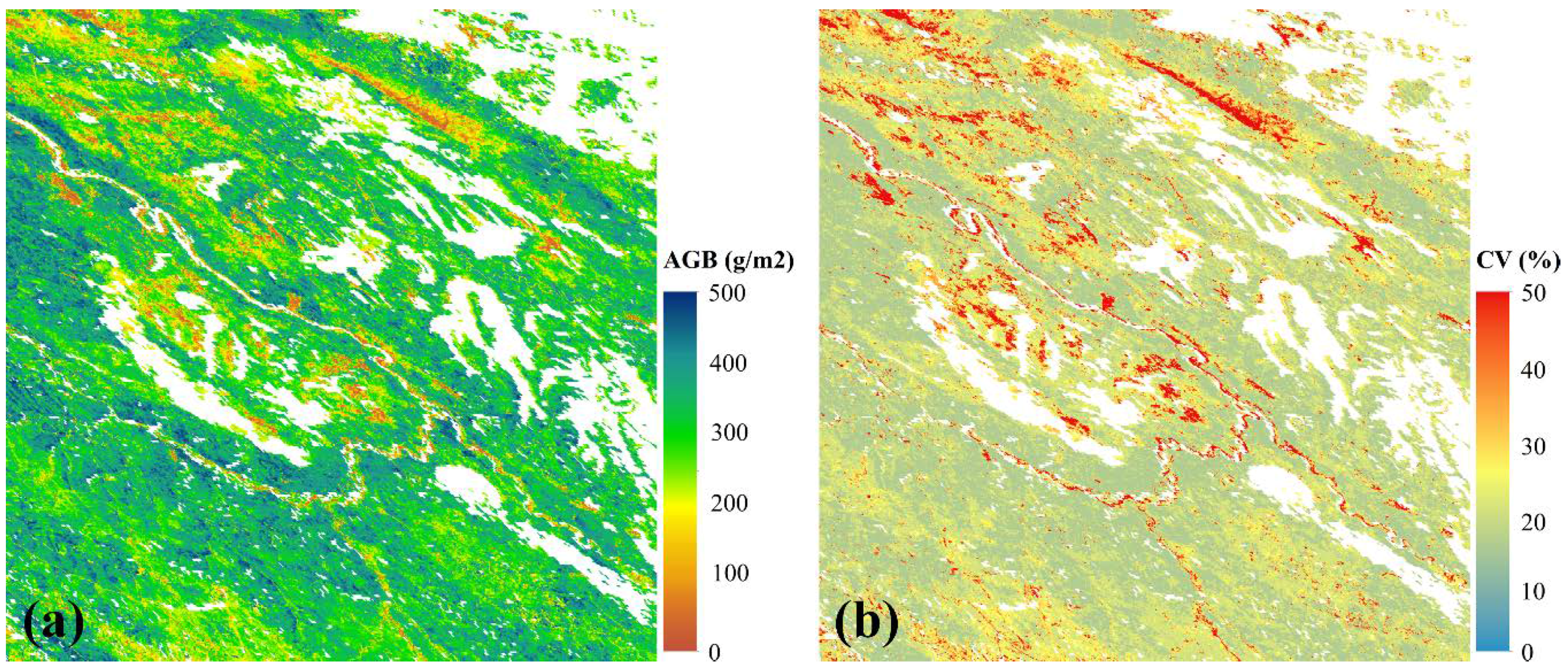
4.3. Aboveground Biomass and Uncertainty Maps
5. Discussion
5.1. Gap Filling for Grassland AGB Estimation
5.2. Benefits from GPR
5.3. Selection of Vegetation Indices
6. Conclusions
Author Contributions
Funding
Conflicts of Interest
References
- Scurlock, J.M.O.; Hall, D.O. The global carbon sink: A grassland perspective. Glob. Chang. Biol. 1998, 4, 229–233. [Google Scholar] [CrossRef]
- Shoko, C.; Mutanga, O.; Dube, T. Progress in the remote sensing of C3 and C4 grass species aboveground biomass over time and space. ISPRS J. Photogramm. Remote Sens. 2016, 120, 13–24. [Google Scholar] [CrossRef]
- Bojinski, S.; Verstraete, M.; Peterson, T.C.; Richter, C.; Simmons, A.; Zemp, M. The concept of essential climate variables in support of climate research, applications, and policy. Bull. Am. Meteorol. Soc. 2014, 95, 1431–1443. [Google Scholar] [CrossRef]
- Yang, Y.H.; Fang, J.Y.; Pan, Y.D.; Ji, C.J. Aboveground biomass in Tibetan grasslands. J. Arid Environ. 2009, 73, 91–95. [Google Scholar] [CrossRef]
- Gao, T.; Yang, X.C.; Jin, Y.X.; Ma, H.L.; Li, J.Y.; Yu, H.D.; Yu, Q.Y.; Zheng, X.; Xu, B. Spatio-Temporal Variation in Vegetation Biomass and Its Relationships with Climate Factors in the Xilingol Grasslands, Northern China. PLoS ONE 2013, 8, e83824. [Google Scholar] [CrossRef] [PubMed]
- Sinha, S.; Jeganathan, C.; Sharma, L.K.; Nathawat, M.S. A review of radar remote sensing for biomass estimation. Int. J. Environ. Sci. Technol. 2015, 12, 1779–1792. [Google Scholar] [CrossRef]
- Greaves, H.E.; Vierling, L.A.; Eitel, J.U.H.; Boelman, N.T.; Magney, T.S.; Prager, C.M.; Griffin, K.L. Estimating aboveground biomass and leaf area of low-stature Arctic shrubs with terrestrial LiDAR. Remote Sens. Environ. 2015, 164, 26–35. [Google Scholar] [CrossRef]
- He, B.B.; Li, X.; Quan, X.W.; Qiu, S. Estimating the aboveground dry biomass of grass by assimilation of retrieved LAI into a crop growth model. IEEE J. Sel. Top. Appl. Earth Obs. Remote Sens. 2015, 8, 550–561. [Google Scholar] [CrossRef]
- Liang, T.G.; Yang, S.X.; Feng, Q.S.; Liu, B.K.; Zhang, R.P.; Huang, X.D.; Xie, H.J. Multi-factor modeling of above-ground biomass in alpine grassland: A case study in the Three-River Headwaters Region, China. Remote Sens. Environ. 2016, 186, 164–172. [Google Scholar] [CrossRef]
- Reddersen, B.; Fricke, T.; Wachendorf, M. A multi-sensor approach for predicting biomass of extensively managed grassland. Comput. Electron. Agric. 2014, 109, 247–260. [Google Scholar] [CrossRef]
- Quan, X.W.; He, B.B.; Yebra, M.; Yin, C.M.; Liao, Z.M.; Zhang, X.T.; Li, X. A radiative transfer model-based method for the estimation of grassland aboveground biomass. Int. J. Appl. Earth Obs. Geoinf. 2017, 54, 159–168. [Google Scholar] [CrossRef]
- Sibanda, M.; Mutanga, O.; Rouget, M. Examining the potential of Sentinel-2 MSI spectral resolution in quantifying above ground biomass across different fertilizer treatments. ISPRS J. Photogramm. Remote Sens. 2015, 110, 55–65. [Google Scholar] [CrossRef]
- Li, F.; Zeng, Y.; Luo, J.H.; Ma, R.H.; Wu, B.F. Modeling grassland aboveground biomass using a pure vegetation index. Ecol. Indic. 2016, 62, 279–288. [Google Scholar] [CrossRef]
- Ullah, S.; Si, Y.; Schlerf, M.; Skidmore, A.K.; Shafique, M.; Iqbal, I.A. Estimation of grassland biomass and nitrogen using MERIS data. Int. J. Appl. Earth Obs. Geoinf. 2012, 19, 196–204. [Google Scholar] [CrossRef]
- Dusseux, P.; Hubert-Moy, L.; Corpetti, T.; Vertès, F. Evaluation of SPOT imagery for the estimation of grassland biomass. Int. J. Appl. Earth Obs. Geoinf. 2015, 38, 72–77. [Google Scholar] [CrossRef]
- Liu, S.L.; Cheng, F.Y.; Dong, S.K.; Zhao, H.D.; Hou, X.Y.; Wu, X. Spatiotemporal dynamics of grassland aboveground biomass on the Qinghai-Tibet Plateau based on validated MODIS NDVI. Sci. Rep. 2017, 7, 4182. [Google Scholar] [CrossRef] [PubMed]
- Piao, S.L.; Fang, J.Y.; Zhou, L.M.; Tan, K.; Tao, S. Changes in biomass carbon stocks in China's grasslands between 1982 and 1999. Glob. Biogeochem. Cycles 2007, 21, GB2002. [Google Scholar] [CrossRef]
- Jia, W.X.; Liu, M.; Yang, Y.H.; He, H.L.; Zhu, X.D.; Yang, F.; Yin, C.; Xiang, W.N. Estimation and uncertainty analyses of grassland biomass in Northern China: Comparison of multiple remote sensing data sources and modeling approaches. Ecol. Indic. 2016, 60, 1031–1040. [Google Scholar] [CrossRef]
- Verrelst, J.; Alonso, L.; Camps-Valls, G.; Delegido, J.; Moreno, J. Retrieval of vegetation biophysical parameters using Gaussian process techniques. IEEE Trans. Geosci. Remote Sens. 2012, 50, 1832–1843. [Google Scholar] [CrossRef]
- Xie, Y.C.; Sha, Z.Y.; Yu, M.; Bai, Y.F.; Zhang, L. A comparison of two models with Landsat data for estimating above ground grassland biomass in Inner Mongolia, China. Ecol. Model. 2009, 220, 1810–1818. [Google Scholar] [CrossRef]
- Fang, H.L.; Liang, S.L.; Townshend, J.R.; Dickinson, R.E. Spatially and temporally continuous LAI data sets based on an integrated filtering method: Examples from North America. Remote Sens. Environ. 2008, 112, 75–93. [Google Scholar] [CrossRef]
- Camps-Valls, G.; Gómez-Chova, L.; Muñoz-Marí, J.; Vila-Francés, J.; Amorós, J.; Valle-Tascon, S.D.; Calpe-Maravilla, J. Biophysical parameter estimation with adaptive Gaussian processes. In Proceedings of the 2009 IEEE International Geoscience and Remote Sensing Symposium (IGARSS 2009), Cape Town, South Africa, 12–17 July 2009; pp. 69–72. [Google Scholar]
- Rasmussen, C.E.; Williams, C.K. Gaussian Processes for Machine Learning; The MIT Press: Cambridge, MA, USA, 2006; Volume 2, p. 4. [Google Scholar]
- Verrelst, J.; Rivera, J.P.; Moreno, J.; Camps-Valls, G. Gaussian processes uncertainty estimates in experimental Sentinel-2 LAI and leaf chlorophyll content retrieval. ISPRS J. Photogramm. Remote Sens. 2013, 86, 157–167. [Google Scholar] [CrossRef]
- Mousivand, A.; Menenti, M.; Gorte, B.; Verhoef, W. Multi-temporal, multi-sensor retrieval of terrestrial vegetation properties from spectral-directional radiometric data. Remote Sens. Environ. 2015, 158, 311–330. [Google Scholar] [CrossRef]
- Bazi, Y.; Alajlan, N.; Melgani, F.; AlHichri, H.; Yager, R.R. Robust estimation of water chlorophyll concentrations with Gaussian process regression and IOWA aggregation operators. IEEE J. Sel. Top. Appl. Earth Obs. Remote Sens. 2014, 7, 3019–3028. [Google Scholar] [CrossRef]
- Gao, F.; Masek, J.; Schwaller, M.; Hall, F. On the blending of the Landsat and MODIS surface reflectance: Predicting daily Landsat surface reflectance. IEEE Trans. Geosci. Remote Sens. 2006, 44, 2207–2218. [Google Scholar]
- Zhu, X.; Helmer, E.H.; Gao, F.; Liu, D.; Chen, J.; Lefsky, M.A. A flexible spatiotemporal method for fusing satellite images with different resolutions. Remote Sens. Environ. 2016, 172, 165–177. [Google Scholar] [CrossRef]
- Yin, G.F.; Li, A.N.; Jin, H.A.; Zhao, W.; Bian, J.H.; Qu, Y.H.; Zeng, Y.L.; Xu, B.D. Derivation of temporally continuous LAI reference maps through combining the LAINet observation system with CACAO. Agric. For. Meteorol. 2017, 233, 209–221. [Google Scholar] [CrossRef]
- Zhang, H.K.; Chen, J.M.; Huang, B.; Song, H.H.; Li, Y.R. Reconstructing Seasonal Variation of Landsat Vegetation Index Related to Leaf Area Index by Fusing with MODIS Data. IEEE J. Sel. Top. Appl. Earth Obs. Remote Sens. 2014, 7, 950–960. [Google Scholar] [CrossRef]
- Karnieli, A.; Gabai, A.; Ichoku, C.; Zaady, E.; Shachak, M. Temporal dynamics of soil and vegetation spectral responses in a semi-arid environment. Int. J. Remote Sens. 2002, 23, 4073–4087. [Google Scholar] [CrossRef]
- Chen, J.; Jonsson, P.; Tamura, M.; Gu, Z.H.; Matsushita, B.; Eklundh, L. A simple method for reconstructing a high-quality NDVI time-series data set based on the Savitzky-Golay filter. Remote Sens. Environ. 2004, 91, 332–344. [Google Scholar] [CrossRef]
- Yin, G.; Li, A.; Jin, H.; Bian, J. Spatiotemporal fusion through the best linear unbiased estimator to generate fine spatial resolution NDVI time series. Int. J. Remote Sens. 2018, 39, 3287–3305. [Google Scholar] [CrossRef]
- Verger, A.; Baret, F.; Weiss, M.; Kandasamy, S.; Vermote, E. The CACAO method for smoothing, gap filling, and characterizing seasonal anomalies in satellite time series. IEEE Trans. Geosci. Remote Sens. 2013, 51, 1963–1972. [Google Scholar] [CrossRef]
- Verger, A.; Baret, F.; Weiss, M. Near real-time vegetation monitoring at global scale. IEEE J. Sel. Top. Appl. Earth Obs. Remote Sens. 2014, 7, 3473–3481. [Google Scholar] [CrossRef]
- Li, A.N.; Bian, J.H.; Lei, G.B.; Huang, C.Q. Estimating the maximal light use efficiency for different vegetation through the CASA model combined with time-series remote sensing data and ground measurements. Remote Sens. 2012, 4, 3857–3876. [Google Scholar] [CrossRef]
- Wang, J.Y.; Li, A.N.; Bian, J.H. Simulation of the Grazing Effects on Grassland Aboveground Net Primary Production Using DNDC Model Combined with Time-Series Remote Sensing Data-A Case Study in Zoige Plateau, China. Remote Sens. 2016, 8, 168. [Google Scholar] [CrossRef]
- Vermote, E.; Justice, C.; Claverie, M.; Franch, B. Preliminary analysis of the performance of the Landsat 8/OLI land surface reflectance product. Remote Sens. Environ. 2016, 185, 46–56. [Google Scholar] [CrossRef]
- United States Geological Survey (USGS). Landsat 8 Surface Reflectance Code (LaSRC) Product Guide, USGS: Reston, VA, USA, 2017.
- Schaaf, C.B.; Gao, F.; Strahler, A.H.; Lucht, W.; Li, X.W.; Tsang, T.; Strugnell, N.C.; Zhang, X.Y.; Jin, Y.F.; Muller, J.P.; et al. First operational BRDF, albedo nadir reflectance products from MODIS. Remote Sens. Environ. 2002, 83, 135–148. [Google Scholar] [CrossRef]
- Mutanga, O.; Skidmore, A.K. Narrow band vegetation indices overcome the saturation problem in biomass estimation. Int. J. Remote Sens. 2004, 25, 3999–4014. [Google Scholar] [CrossRef]
- GCOS. Systematic Observation Requirements for Satellite-Based Products for Climate: Supplemental Details to the Satellite-Based Component of the “Implementation Plan for the Global Observing System for Climate in Support of the UNFCCC”; World Meteorological Organization: Geneva, Switzerland, 2011; p. 89. [Google Scholar]
- Yin, G.F.; Li, J.; Liu, Q.H.; Li, L.H.; Zeng, Y.L.; Xu, B.D.; Yang, L.; Zhao, J. Improving leaf area index retrieval over heterogeneous surface by integrating textural and contextual information: A case study in the Heihe River Basin. IEEE Geosci. Remote Sens. Lett. 2015, 12, 359–363. [Google Scholar]
- Savoy, P.; Mackay, D.S. Modeling the seasonal dynamics of leaf area index based on environmental constraints to canopy development. Agric. For. Meteorol. 2015, 200, 46–56. [Google Scholar] [CrossRef]
- Verrelst, J.; Pablo Rivera, J.; Veroustraete, F.; Munoz-Mari, J.; Clevers, J.G.P.W.; Camps-Valls, G.; Moreno, J. Experimental Sentinel-2 LAI estimation using parametric, non-parametric and physical retrieval methods—A comparison. ISPRS J. Photogramm. Remote Sens. 2015, 108, 260–272. [Google Scholar] [CrossRef]
- Scholze, M.; Buchwitz, M.; Dorigo, W.; Guanter, L.; Shaun, Q.G. Reviews and syntheses: Systematic Earth observations for use in terrestrial carbon cycle data assimilation systems. Biogeosciences 2017, 14, 3401–3429. [Google Scholar] [CrossRef]
- Ramoelo, A.; Cho, M.A.; Mathieu, R.; Madonsela, S.; van de Kerchove, R.; Kaszta, Z.; Wolff, E. Monitoring grass nutrients and biomass as indicators of rangeland quality and quantity using random forest modelling and World View-2 data. Int. J. Appl. Earth Obs. Geoinf. 2015, 43, 43–54. [Google Scholar] [CrossRef]
- Fu, X.Y.; Tang, C.J.; Zhang, X.X.; Fu, J.Y.; Jiang, D. An improved indicator of simulated grassland production based on MODIS NDVI and GPP data: A case study in the Sichuan province, China. Ecol. Indic. 2014, 40, 102–108. [Google Scholar] [CrossRef]


© 2018 by the author. Licensee MDPI, Basel, Switzerland. This article is an open access article distributed under the terms and conditions of the Creative Commons Attribution (CC BY) license (http://creativecommons.org/licenses/by/4.0/).
Share and Cite
Yin, G.; Li, A.; Wu, C.; Wang, J.; Xie, Q.; Zhang, Z.; Nan, X.; Jin, H.; Bian, J.; Lei, G. Seamless Upscaling of the Field-Measured Grassland Aboveground Biomass Based on Gaussian Process Regression and Gap-Filled Landsat 8 OLI Reflectance. ISPRS Int. J. Geo-Inf. 2018, 7, 242. https://doi.org/10.3390/ijgi7070242
Yin G, Li A, Wu C, Wang J, Xie Q, Zhang Z, Nan X, Jin H, Bian J, Lei G. Seamless Upscaling of the Field-Measured Grassland Aboveground Biomass Based on Gaussian Process Regression and Gap-Filled Landsat 8 OLI Reflectance. ISPRS International Journal of Geo-Information. 2018; 7(7):242. https://doi.org/10.3390/ijgi7070242
Chicago/Turabian StyleYin, Gaofei, Ainong Li, Chaoyang Wu, Jiyan Wang, Qiaoyun Xie, Zhengjian Zhang, Xi Nan, Huaan Jin, Jinhu Bian, and Guangbin Lei. 2018. "Seamless Upscaling of the Field-Measured Grassland Aboveground Biomass Based on Gaussian Process Regression and Gap-Filled Landsat 8 OLI Reflectance" ISPRS International Journal of Geo-Information 7, no. 7: 242. https://doi.org/10.3390/ijgi7070242
APA StyleYin, G., Li, A., Wu, C., Wang, J., Xie, Q., Zhang, Z., Nan, X., Jin, H., Bian, J., & Lei, G. (2018). Seamless Upscaling of the Field-Measured Grassland Aboveground Biomass Based on Gaussian Process Regression and Gap-Filled Landsat 8 OLI Reflectance. ISPRS International Journal of Geo-Information, 7(7), 242. https://doi.org/10.3390/ijgi7070242