Implementation of a Parallel GPU-Based Space-Time Kriging Framework

Abstract

In the study of spatiotemporal geographical phenomena, the space–time interpolation method is widely applied, and the demands for computing speed and accuracy are increasing. For nonprofessional modelers, utilizing the space–time interpolation method quickly is a challenge. To solve this problem, the classical ordinary kriging algorithm was selected and expanded to a spatiotemporal kriging algorithm. Using the OpenCL framework to integrate central processing unit (CPU) and graphic processing unit (GPU) computing resources, a parallel spatiotemporal kriging algorithm was implemented, and three experiments were conducted in this work to verify the results. The results indicated the following: (1) when the size of the prediction point dataset is consistent, the performance of the method is robust with the increasing size of the observation point dataset; (2) the acceleration effect of the parallel method increases with an increased number of predicted points. Compared with the original sequential program, the implementation of the improved parallel framework showed a 3.23 speedup, which obviously shortens the interpolation time; (3) when cross-validating the temperature data in the Beijing Tianjin Hebei region, the space–time acceleration model provides a better fit than traditional pure space interpolation.

1. Introduction

A variety of spatial interpolation methods have been proposed to allow better understanding of the spatial distribution of an area covered by existing observed points. Basically, spatial interpolation becomes a standard tool for geographic information system (GIS) software and plays an important role in Digital Earth (DE) research [1]. Due to the continuous accumulation of historical data and the societal need for the analysis of variables that vary in space and time, such as weather and air quality variables, the collection and processing of spatiotemporal data is rapidly increasing [2]. Researchers have begun to pay attention to the space–time interpolation problem to estimate the spatial and temporal variation characteristics of various spatial elements after time dimension integration and to provide support for decision-making. In recent years, the theoretical aspects of spatiotemporal geostatistics have made great progress [3], but there are still some application problems. Spatiotemporal models are more complex than pure spatial models, and the operations involved in spatiotemporal models are much more expensive.

For these reasons, many scholars have studied the space–time interpolation problem. With the help of existing methods, some scholars have tried to improve time and space interpolations. For example, the kriging method is used for the best, unbiased, optimal estimation of regionalized sampling point variables using the structural features of observations with known spatial distributions. Although originally developed for geostatistics, the kriging method is now widely used in geology [4], hydrology [5], meteorology [6], environmental science [7] and other disciplines. However, in the real world, many geographical phenomena have temporal and spatial evolution processes. As a spatial interpolation method, kriging often ignores the important information about the time dimension in the problem, which is not conducive to further improving the accuracy of the interpolation.

Through the evolution of regionalized variables into spatiotemporal regionalized variables, scholars established spatiotemporal variogram models [8], which can achieve the spatial and temporal extension of kriging interpolation. To date, spatiotemporal kriging interpolation has been applied in many fields. Raja et al. [9] used spatiotemporal kriging interpolation to research the trends of spatiotemporal variation in regional precipitation, which can be used to plan and manage water resources in areas that are heavily dependent on precipitation. Yang et al. [10,11] assessed the sources and spatiotemporal trends of heavy metal accumulation in soil using the spatiotemporal kriging method and provided suggestions for the prevention and control of heavy metal pollution in soil. Jost et al. [12,13] used an interpolation method to determine the distribution of a forest ecosystem and the water storage layer near the desert; their method can assist groundwater managers to make correct decisions. Park et al. [14,15] used the spatiotemporal kriging method to more accurately estimate the spread of air pollutants and the distribution of infectious diseases, adding to omissions in the data collection process.

With the expansion of interpolation algorithms in the time dimension, it is necessary to acquire sample points at different times and to obtain the time trend of the study area. As a result, the number of sampling points increases linearly and interpolation algorithms require large computation and storage resources; the algorithms are slow and inefficient on traditional personal computers (PCs), which is not conducive to the use of applications.

With the development of computing technology, high-performance computing (HPC) technology has been gradually integrated into the field of geographic information, which has improved the application, promotion and development of the field. Multiple processors, parallel clustering, grid computing, graphic processing unit (GPU) incorporation and other high-performance computing technologies have attracted much research attention in the geosciences field [16,17,18]. In recent years, parallel computing has mainly appeared in the form of multi-core processors [19]. A GPU has a large number of cores, which makes up for the shortcomings of the traditional central processing unit (CPU) architecture.

High-performance GIS computing algorithms are a research hotspot that is mainly divided into two aspects. One aspect is the optimization of processing from the technical level, parallel to existing high-density computing, to improve operational efficiency. The second aspect is the exploration of a new spatiotemporal analysis model using modeling and algorithms to develop a more efficient and convenient spatiotemporal analysis model.

To represent the spatial interpolation model by the kriging interpolation method in the technical level of optimization and new space interpolation algorithm improvement, scholars have begun to use GPUs to reduce computing time and introduce mature parallelization schemes. Cheng [20] accelerated the universal kriging algorithm on the NVIDIA Compute Unified Device Architecture (CUDA) platform and achieved a nearly 18-fold speed increase with respect to the sequential program. Liu [21] used the computation power of modern programmable graphics hardware (GPU) for 3D visualization in a reservoir modeling system. In terms of algorithms and model improvements, Liu [22] proposed an algorithm based on the k-d tree method to address the unevenly distributed spatial data. Hu et al. [23] proposed an fast Fourier transform (FFT)-based parallel algorithm to accelerate regression kriging interpolation, which was computed on a GPU device. As far as we know, spatiotemporal kriging is an improved method for spatiotemporal interpolation; however, the model and the algorithm have changed, and the original parallel method cannot adapt.

Although many people pay attention to the general spatial analysis of GIS, the support of spatiotemporal interpolation and efficiency improvement calculations lack in-depth research. To solve the above problems, the spatiotemporal kriging algorithm was analyzed, data associations were decoupled and parallelized, and a parallel algorithm of spatiotemporal kriging interpolation was proposed. The parallel model of the space–time interpolation is tested with meteorological data in this paper. The purpose of this paper is to propose a new space–time interpolation algorithm and technology supported by HPC, which will provide new research ideas for GIS spatiotemporal analysis modeling and the enrichment of GIS research contents.

This article is arranged as follows: in the first and second parts of Section 2, we introduce the spatiotemporal kriging algorithm and the space–time extension in detail. The third part of Section 2 focuses on the design of the parallel spatiotemporal kriging algorithm and implementation by the OpenCL framework. In Section 3, the experimental results and analysis are given. Section 4 presents the conclusion.

2. Methodology and Implementation

Similar to spatial interpolation, spatiotemporal geostatistics need are dependent on a suitable spatiotemporal covariance model [24]. Many kinds of models have been designed, including linear, separable and nonseparable models [25,26,27]. We aimed to implement space–time interpolation using a product–sum model with the support of HPC. Other types of interpolation methods can be properly extended or adjusted on the basis of this method. The data selected in this article are meteorological data. Ordinary kriging interpolation can meet the needs of homogeneous regions. Therefore, ordinary kriging interpolation was used in the experiment.

2.1. Ordinary Kriging

The kriging method makes an unbiased, optimal estimation of the regionalized variables of the sampling points and uses a semi-variogram to represent the structural features of the region. Kriging is a linear interpolation method. Using the obtained spatial structure and the known sampling points to predict results, we can use Equation (1):

$$\widehat{Z}{s}_0={\displaystyle \sum }_{i=1}^N{\lambda }_{i}Z\left(s_i\right),$$

(1)

where $\widehat{Z}{s}_0$ is the estimated value, $Z\left(s_i\right)$ refers to each known point, $N$ is the measured value number and ${\lambda }_i$ is the weight value at the position.

The ordinary kriging assumption is that the estimator expected value is equal to the true value, and the prediction error variance is minimized. Therefore, to ensure the best linear unbiased prediction of the prediction point, the sum of the weight coefficients of the surrounding sampling points must be equal to 1. This process can be represented by kriging Equation (2):

$$\left[\begin{array}{cccc}{\gamma }_{11}& \cdots & {\gamma }_{1N}& 1\\ ⋮& \ddots & ⋮& ⋮\\ {\gamma }_{N1}& \cdots & {\gamma }_{NN}& 1\\ 1& 1& 1& 0\end{array}\right]\times \left[\begin{array}{c}{\lambda }_1\\ ⋮\\ {\lambda }_N\\ \mu \end{array}\right]=\left[\begin{array}{c}{\gamma }_{10}\\ ⋮\\ {\gamma }_{N0}\\ 1\end{array}\right],$$

(2)

where ${\gamma }_{11}$ stands for the variogram value between point $i$ and point $j$, and μ is a Lagrange multiplier.

2.2. Spatiotemporal Kriging Algorithm

The spatiotemporal kriging interpolation method is used to extend the time dimension to the kriging interpolation. The regionalized variables are evolved into spatiotemporal regionalized variables, and the spatiotemporal variogram model is used to fit the sampling points. The relationship between the variogram and covariance is:

$${\gamma }_s\left(h_s\right)=C_s\left(0\right)-C_s\left(h_s\right),$$

(3)

$${\gamma }_t\left(h_t\right)=C_t\left(0\right)-C_t\left(h_t\right),$$

(4)

$${\gamma }_{st}\left(h_s,h_t\right)=C_{st}\left(0,0\right)-C_{st}\left(h_s,h_t\right),$$

(5)

where ${\gamma }_s\left(h_s\right)$, ${\gamma }_t\left(h_t\right)$, and ${\gamma }_{st}\left(h_s,h_t\right)$ are the spatial, temporal, and spatiotemporal variograms, $C_s\left(h_s\right)$, $C_t\left(h_t\right)$, and $C_{st}\left(h_s,h_t\right)$ are the spatial, temporal, and spatiotemporal covariance functions, and $h_{s }$ and $h_t$ are space and time distances, respectively.

Due to the different dimensions of the spatial domain and the time domain, the spatial and temporal variograms are difficult to calculate directly. According to a type of product–sum model [28], the sum–product model of space–time covariance function is defined as Equation (6):

$$C_{st}\left(h_s,h_t\right)=k_1{C}_s\left(h_s\right)C_t\left(h_t\right)+k_2{C}_s\left(h_s\right)+k_3{C}_t\left(h_t\right).$$

(6)

The introduction of $k_1$, $k_2$ and $k_3$ ensures the positivity of the space–time covariance function, $C_{st}\left(h_s,h_t\right)$. Where $h_s$ = 0, $h_t$ = 0 can be obtained from Equation (7):

$$C_{st}\left(0,0\right)=k_1{C}_s\left(0\right)C_t\left(0\right)+k_2{C}_s\left(0\right)+k_3{C}_t\left(0\right).$$

(7)

$C_{st}\left(0,0\right), C_s\left(0\right),$ and $C_t\left(0\right)$ are the nugget values of space, time and space–time, respectively. Using the above equations, the spatiotemporal variogram is obtained (Equation (8)):

$${\gamma }_{st}\left(h_s,h_t\right)=\left(k_1{C}_t\left(0\right)+k_2\right){\gamma }_s\left(h_s\right)+\left(k_1{C}_s\left(0\right)+k_3\right){\gamma }_t\left(h_t\right)-k_1{\gamma }_s\left(h_s\right){\gamma }_t\left(h_t\right).$$

(8)

According to ordinary kriging prediction formula, the ordinary spatiotemporal kriging interpolation is obtained with Equation (9):

$$Z^{*}\left(s_0,t_0\right)={\displaystyle \sum }_{i=1}^n{\displaystyle \sum }_{j=1}^m{\lambda }_{\left(i,j\right)}Z\left(s_i,t_j\right).$$

(9)

The number of spatial sampling points is i = 1, 2... n, the time sampling points are j = 1, 2, ... m, and the total number of samples is n × m. Z*(s₀, t₀) is the linear estimation of the interpolation point $\left(s_0,t_0\right)$. $Z\left(s_i,t_j\right)$ is the value of the neighboring sampling point $\left(s_i,t_j\right)$. ${\lambda }_{\left(i,j\right)}$ is the weighting coefficient of the point and the kriging model in Equation (10):

$$\left[\begin{array}{c}K\end{array}\right]\times \left[\begin{array}{c}\lambda \end{array}\right]=\left[\begin{array}{c}M\end{array}\right],$$

(10)

$$\left[K\right]=\left|\begin{array}{cccccccc}{\gamma }_{11,11}& {\gamma }_{12,11}& \cdots & {\gamma }_{1n,11}& {\gamma }_{11,12}& \cdots & {\gamma }_{1n,1m}& 1\\ {\gamma }_{21,11}& {\gamma }_{22,11}& \cdots & {\gamma }_{2n,11}& {\gamma }_{21,12}& \cdots & {\gamma }_{2n,1m}& 1\\ \cdots & \cdots & \cdots & \cdots & \cdots & \cdots & \cdots & \cdots \\ {\gamma }_{n1,11}& {\gamma }_{n2,11}& \cdots & {\gamma }_{nn,11}& {\gamma }_{n1,12}& \cdots & {\gamma }_{nn,1m}& 1\\ {\gamma }_{11,21}& {\gamma }_{12,21}& \cdots & {\gamma }_{1n,21}& {\gamma }_{11,22}& \cdots & {\gamma }_{1n,2m}& 1\\ \cdots & \cdots & \cdots & \cdots & \cdots & \cdots & \cdots & \cdots \\ {\gamma }_{n1,m1}& {\gamma }_{n2,m1}& \cdots & {\gamma }_{nn,m1}& {\gamma }_{n1,m2}& \cdots & {\gamma }_{nn,mm}& 1\\ 1& 1& \cdots & 1& 1& \cdots & 1& 0\end{array}\right|,$$

(11)

$$\left[\begin{array}{c}M\end{array}\right]={\left[{\gamma }_{\left(01,01\right)}, {\gamma }_{\left(02,01\right)}, \dots , {\gamma }_{\left(0n,01\right)}, {\gamma }_{\left(01,02\right)}, \dots , {\gamma }_{\left(0n,0m\right)}, 1\right]}^T,$$

(12)

$$\left[\begin{array}{c}\lambda \end{array}\right]={\left[{\lambda }_{\left(1,1\right)}, {\lambda }_{\left(2,1\right)}, \dots , {\lambda }_{\left(n,1\right)},{\lambda }_{\left(1,2\right)}, \dots , {\lambda }_{\left(n,m\right)}, \mu \right]}^T.$$

(13)

Specifically, the serial algorithm of the ordinary spatiotemporal kriging interpolation consists of the following four steps:

• Step 1: Calculate the variograms of the pure time domain and the pure space domain and fit them. At different time points, the space point has a different nugget, sill and range. Calculate the average $C_{st}\left(0,0\right),C_s\left(0\right),$ and $C_t\left(0\right)$ here.
• Step 2: Based on the results of Step (1), ${\gamma }_s\left(h_s\right)$ and ${\gamma }_t\left(h_t\right)$ are constructed. Substituting $k_1, k_2, k_3, {\gamma }_s\left(h_s\right)$ and ${\gamma }_t\left(h_t\right)$ into Equation (8), we get the spatiotemporal variograms, ${\gamma }_{st}\left(h_s,h_t\right)$.
• Step 3: Calculate the space–time distance between the point to be measured and the surrounding points (known points, where the sum is $n$ × $m$), i.e., $d_1$, $d_2$, …, $d_n$, $t_1$, $t_2$, …, $t_n$. Obtain the variogram vector (Equation (12)).
• Step 4: Bring the known points and the spatiotemporal variogram ${\gamma }_{st}\left(h_s,h_t\right)$ into the kriging equations to obtain the weight vector, and then calculate the estimation of an unobserved point.

2.3. Parallel Ordinary Spatiotemporal Kriging Algorithm Design and Implementation with OpenCL

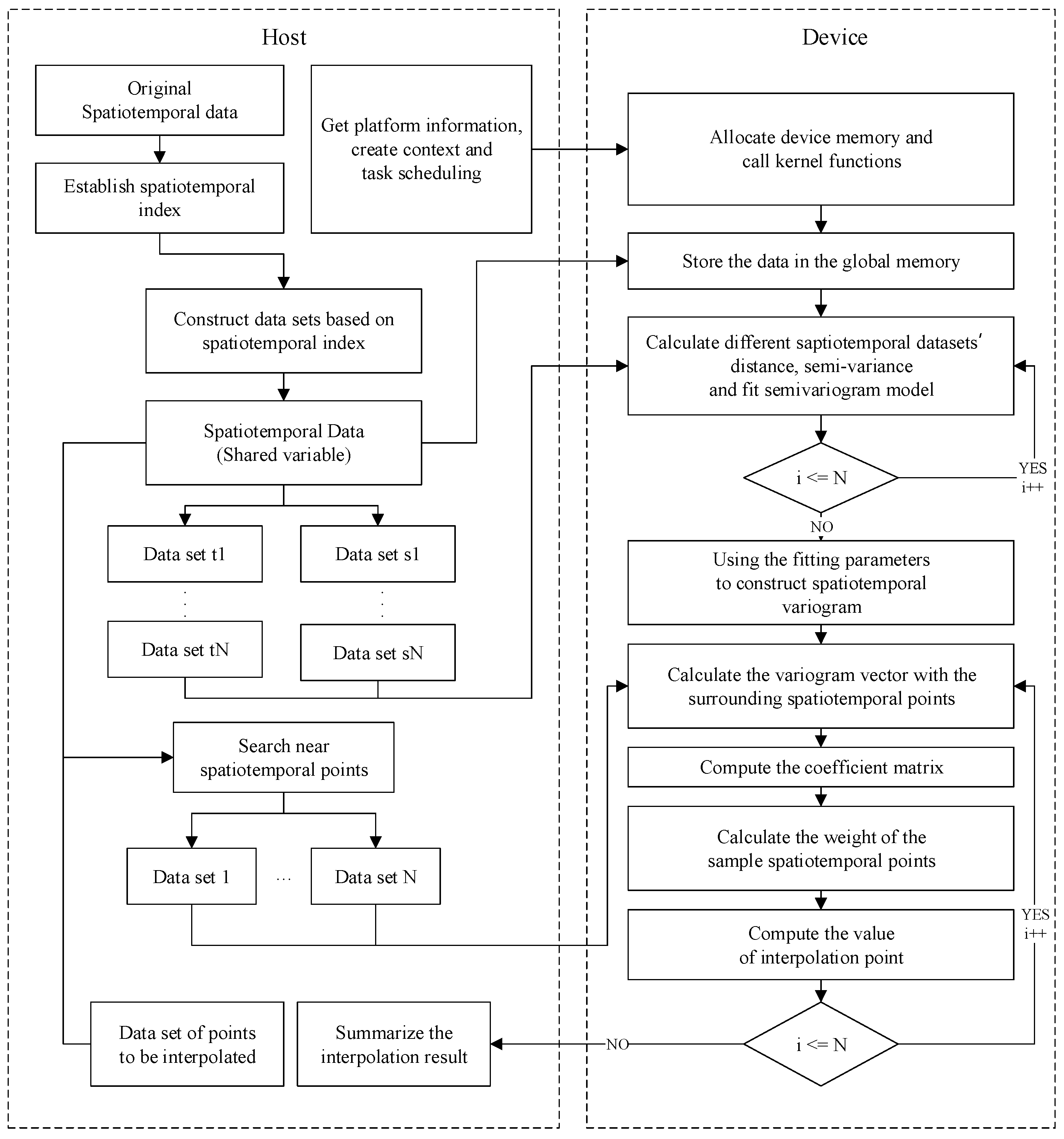
2.3.1. Design and Framework of the Parallel Algorithm

The spatiotemporal kriging interpolation predicts the interpolation points using the structural features of spatiotemporal sample points. According to the principle of the ordinary spatiotemporal kriging algorithm, the algorithm can be divided into the following four steps:

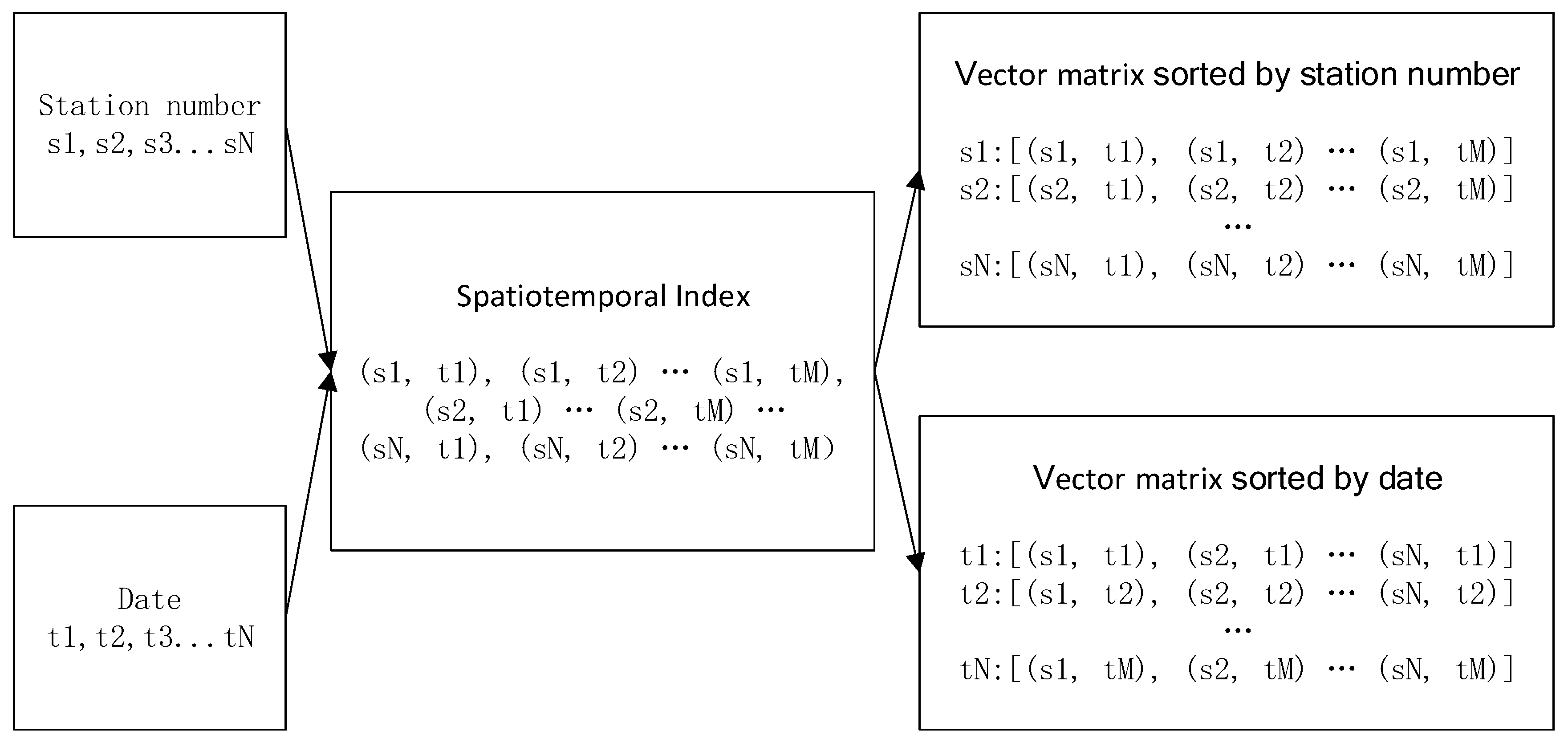
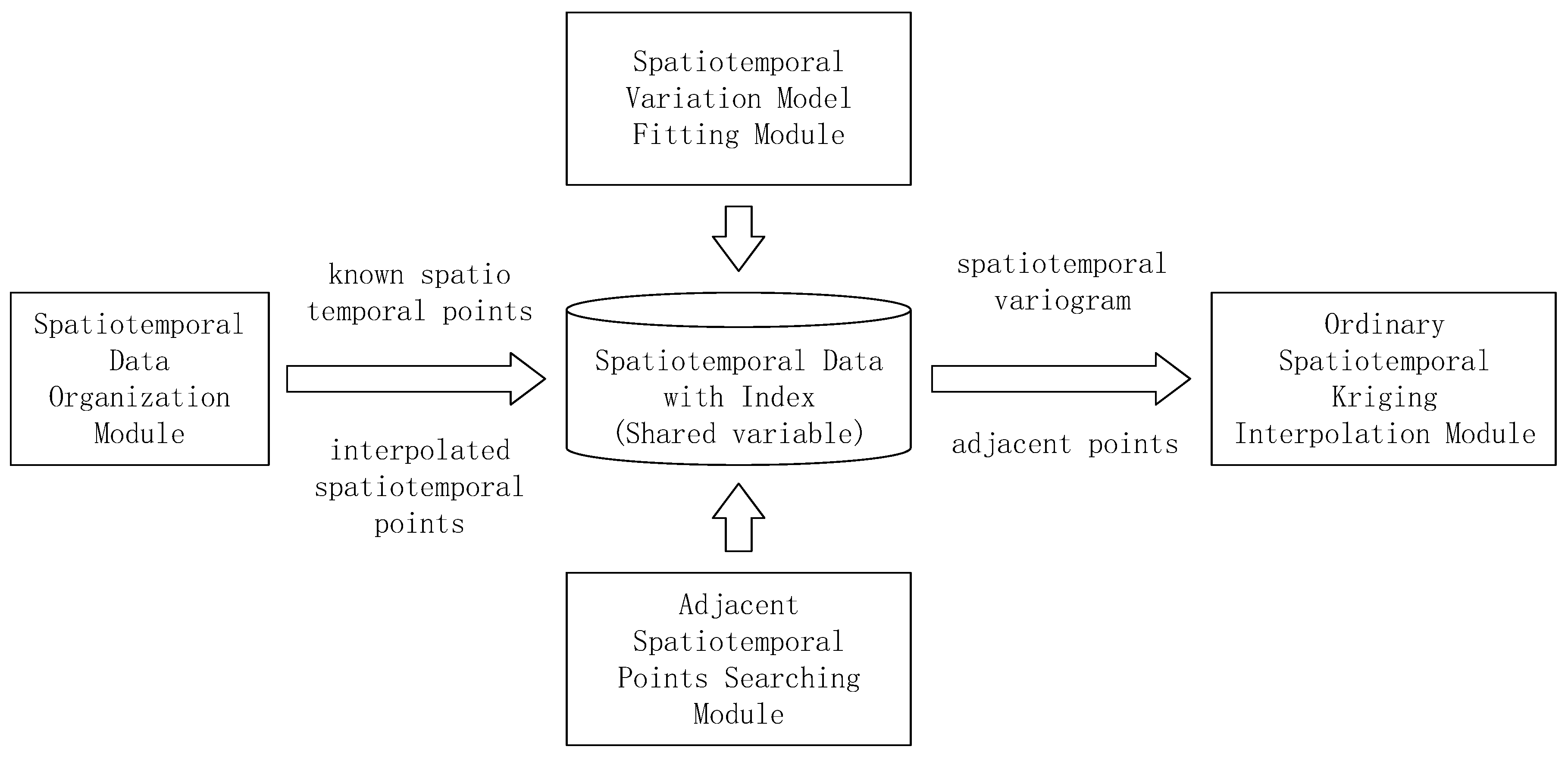
• Step 1: Organize the original data and establish the index to facilitate the query retrieval (Spatiotemporal Data Organization Module, STDOM).
• Step 2: Fit the spatiotemporal variation model of the sample data to obtain the variogram, ${\gamma }_{st},$ of the spatiotemporal structure of the representative sample (Spatiotemporal Variation Model Fitting Module, STVMFM).
• Step 3: Proceed with the set of points to be predicted, search for the adjacent spatiotemporal points and set up the data sets (Adjacent Spatiotemporal Points Searching Module).
• Step 4: Use the spatiotemporal variogram, ${\gamma }_{st}$, and the data sets of the neighboring points for the ordinary spatiotemporal kriging interpolation to calculate the estimated values of the unknown points (Ordinary Spatiotemporal Kriging Interpolation Module, OSTKIM), as shown in Figure 1.

1. Spatiotemporal Data Organization Module (STDOM)

Spatiotemporal data have space coordinates and time information. In the spatiotemporal kriging interpolation algorithm, it is necessary to search for the points neighboring an unknown point in the spatiotemporal sample data. To facilitate this process, an STDOM was designed to index the data. The spatiotemporal index numbered all space points, and then the station number and date were cross-referenced to obtain the index values shown in

Table 1. Definition of the spatiotemporal index.

Station Number (${\mathit{s}}_1, {\mathit{s}}_2,\dots$)	Date (${\mathit{t}}_1, {\mathit{t}}_2,\dots$)	Spatiotemporal Index (${\mathit{s}}_1{\mathit{t}}_1, {\mathit{s}}_2{\mathit{t}}_1,\dots$)
00001	201706	00001201706

.

2. Spatiotemporal Variation Model Fitting Module (STVMFM)

STVMFM is designed to fit different time and space variogram models to obtain the average $\overline{{\mathrm{C}}_{\mathrm{s}}}$, $\overline{{\mathrm{C}}_{\mathrm{t}}}$ as the ${\gamma }_s, {\gamma }_t$ parameters and to calculate $k_1, k_2, \mathrm{and}{k}_3$ to construct the spatiotemporal variogram ${\gamma }_{st}$. To fit the model, according to the spatiotemporal index, data must be divided into the vector matrix of the same time and the vector matrix of the same space (Figure 2). Each vector in the vector matrix is a set of sample points in time or space. Since the solution to the spatiotemporal parameters of each vector is independent, this step can be parallelized.

3. Adjacent Spatiotemporal Points Searching Module (ASTPSM)

The amount of data for space–time interpolation is much greater than that for the pure spatial interpolation. Therefore, instead of using all the sample points, the points in a certain spatiotemporal range are calculated according to the arrangement obtained by fitting of the variation model. In ASTPSM, using the spatiotemporal index established before, a neighbor points search method based on the KD-tree is used. The KD-tree algorithm is used to find the adjacent station number in the neighborhood and this is crossed over with the neighboring date to obtain the target index.

4. Ordinary Spatiotemporal Kriging Interpolation Module (OSTKIM)

The OSTKIM module was used to calculate Equation (9). Parallel calculation of the matrix can greatly speed up the interpolation process. In this step, the coefficient matrix $\left[\begin{array}{c}K\end{array}\right]$ needs to be inversed, and the weight vector $\left[\begin{array}{c}\lambda \end{array}\right]$ is calculated by matrix-vector multiplication. Much progress has been made on the parallelization of matrix operations. Here, an efficient solution that decomposes the coefficient matrix into a lower triangular matrix and an upper triangular matrix by LU decomposition has been chosen before solving a linear system. Then, the system of linear equation decomposition is solved directly by forward and backward substitution without directly calculating the inverse matrix.

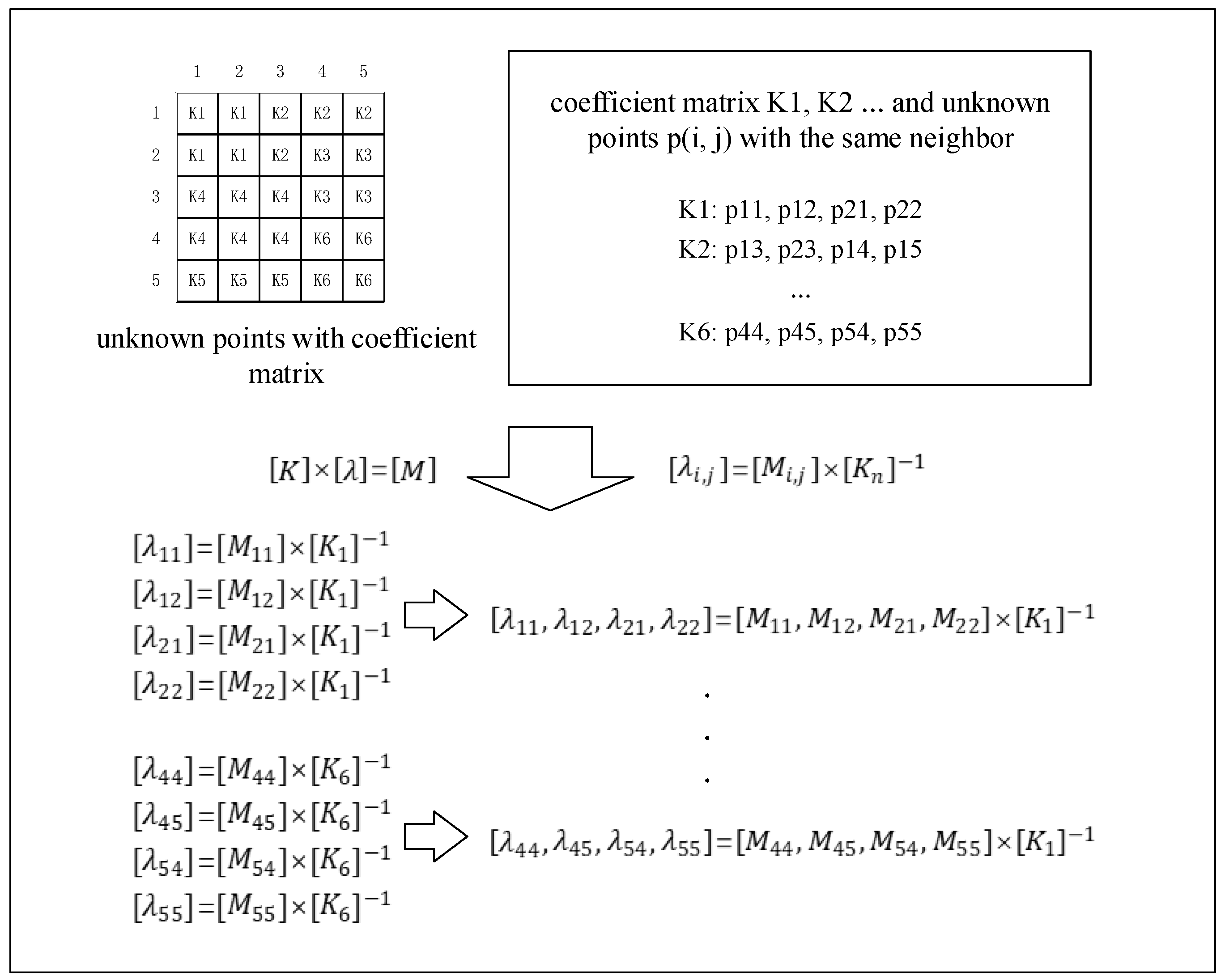
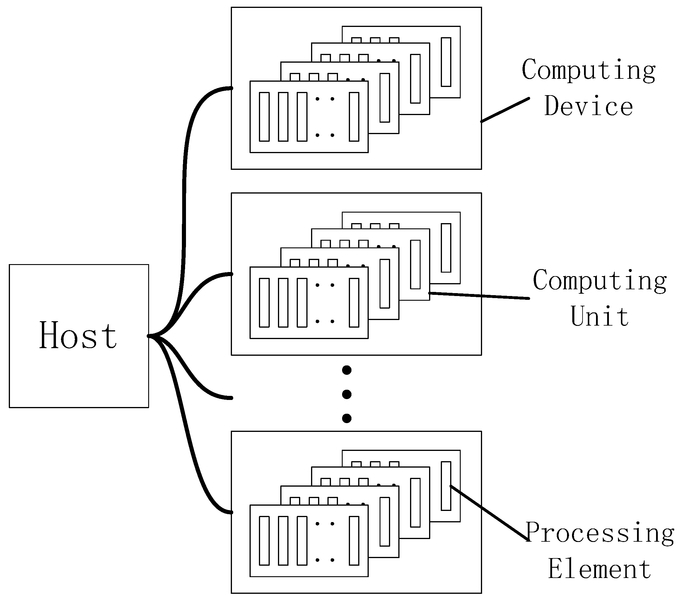
2.3.2. OpenCL-Based Implementation

Open Computing Language (OpenCL) is a framework for writing programs on heterogeneous platforms [29]. OpenCL assumes that computing systems consist of multiple computing devices, which can be central processing units (CPUs) or hardware accelerators, such as graphics processing units (GPUs) connected to a host processor. OpenCL provides a standard interface for parallel computing based on task and data parallelism, as shown in Figure 3:

The OpenCL execution model consists of the following two components: the host program and the kernel. The host program is executed on the host to define the device context, queue the kernel, and execute kernel instances using the command queue. The kernel is an executable code based on the OpenCL standard that runs on the computing device, similar to data or task-parallel functions. In the spatiotemporal kriging interpolation, the calculation of each vector in the STVMFM and the solution to each unknown point in the OSTKIM are independent. So, parallel kernel functions are written, the calculation is distributed to computing devices, and the computing speed is improved.

As the hardware continues to evolve, CPUs and GPUs vary widely in architecture due to their different positioning. Taking the Intel Core i7-7700 and NVIDIA GTX1060 6 G as examples, the former has a base frequency speed of 3.60 GHz and four physical cores with 8 threads per core, and the latter has a base frequency speed of 1.50 GHz with 1280 cores. This shows that the main difference between the two is that the CPU has a faster clock speed and processes a single calculation faster, and the GPU has more cores and is better at handling multiple calculations. Based on these characteristics, this paper implemented the spatiotemporal kriging interpolation algorithm as shown in Figure 4. This algorithm uses the CPU as a host to achieve an STDOM module, an ASTPSM module as well as to create a context, task queue and data division distributed to the computing device. At the same time, the GPU is used as a computing device to achieve an STVMFM module, an OSTKIM module and to speed up the interpolation process.

When using the OSTKIM, the coefficient matrix $\left[\begin{array}{c}K\end{array}\right]$ is the same for the prediction points with the same neighboring points. Memory resources are invaluable in GPU operations. Therefore, for the unknown points that have the same neighboring points, the coefficient matrix $\left[K\right]$ is stored once, and the vectors $\left[\begin{array}{c}M\end{array}\right]$ of the unknown points with the same coefficient matrix are used to construct the matrix for matrix multiplication. This step reduces memory redundancy and avoids high data communication costs, as shown in Figure 5.

3. Experiments and Analysis

3.1. Computational Environment

To facilitate further research, considering the mainstream configuration of computers on the market, we chose the computing platform with the following parameters to carry out the experiment, as shown in

Table 2. Detailed configurations of the experimental platforms.

Platform	Hardware Configuration
Intel® Core™ i7-7700 Processor	Cores: 4
	Threads: 8
	Processor Base Frequency: 3.60 GHz
	Max Turbo Frequency: 4.20 GHz
	Cache: 8 MB Smart Cache
	Bus Speed: 8 GT/s DMI3
Nvidia GeForce GTX 1060	NVIDIA CUDA® Cores: 1280
	Base Clock (MHz): 1506
	Boost Clock (MHz): 1708
	Memory Speed: 8 Gbps
	Standard Memory Config: 6 GB GDDR5
	Memory Bandwidth (GB/sec): 192

.

The experimental data were the monthly average temperatures of 57 sites from 2007 to 2016 in Beijing, Tianjin, Hebei and its surrounding areas (Figure 6), collected by the meteorological data center of the China Meteorological Administration (http://data.cma.cn/data/cdcdetail/dataCode/B.0021.0002.html).

3.2. Experimental Methodology Design

In the above hardware environment, we compared the efficiencies of a CPU sequential program and a GPU-accelerated parallel algorithm. To this end, the following three experiments were designed.

• Experiment 1: four observation point dataset sizes of 2000, 3000, 4000 and 5000 points were used to interpolate a regular grid (1000 × 1000) at a specified time, and the influence of the number of sampling points was tested to determine the algorithm’s efficiency.
• Experiment 2: the dataset of observations with 5000 points was used to determine the effect of the number of interpolation points on the efficiency of the algorithm for the interpolation of five types of prediction point datasets including space images of one moment with resolutions of 500 × 500, 800 × 800, 1000 × 1000 and 2000 × 2000.
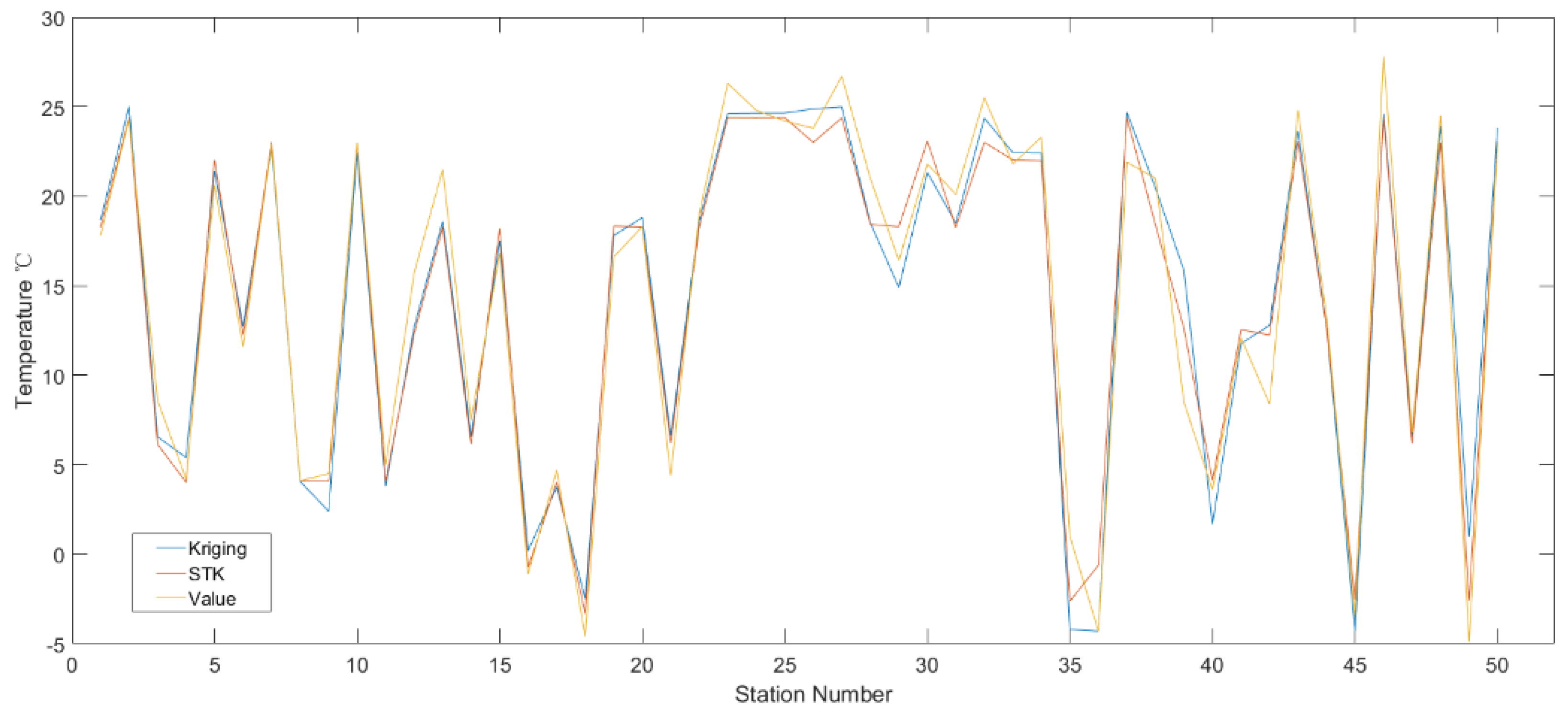
• Experiment 3: the results of the space–time interpolation were verified by cross-validation. The detailed cross-validation process was as follows:
  • Step 1: Delete the first observation value, $Z_1$, from the data set.
  • Step 2: Use other observations, the variogram model and the kriging method to predict the point value, $Z_1^{*}$.
  • Step 3: Put $Z_1$ into the dataset and repeat Step 1 to Step 4 until the other predicted values, $Z_1^{*}, Z_2^{*}, \dots , Z_n^{*}$, are obtained.
  • Step 4: Through comparison of the original data, $\begin{array}{c}{Z}_1,Z_2, \dots , Z_n\end{array}$, and predicted data, $Z_1^{*}, Z_2^{*}, \dots , Z_n^{*}$, the error is calculated, and the effect of interpolation can be judged.

Cross-validation is a gradual process, and the best parameters and variation models can be obtained through many comparisons and practices.

The speed increase was calculated according to Equation (14), and the interpolation performances were compared. $S_p$ is the speed up, $T_1$ represents the run time serial executed by CPU, and $T_2$ is the execution time of the parallel accelerated model in the parallel system. The performance of the proposed parallel algorithm was evaluated with $S_p$:

$$S_p=\frac{T_1}{T_2}.$$

(14)

3.3. Interpolation Acceleration Effect and Analysis

The results of experiment 1 are shown in

Table 3. Comparison of acceleration of different data sizes, the serial spatiotemporal kriging (SSTK) and the parallel spatiotemporal kriging (PSTK).

Observation Datasets	Grid Resolution	SSTK/ms	PSTK/ms	Speed Up
2000	1000 × 1000	25,043	8480	2.95
3000	1000 × 1000	25,654	8718	2.94
4000	1000 × 1000	26,766	8847	3.02
5000	1000 × 1000	27,389	8970	3.05

. As the number of observation points increased, the spatiotemporal kriging parallel algorithm did not significantly increase the time consumption, and the acceleration ratio was approximately 3:1. The parallel interpolation method was able to effectively adapt to changes in the number of sampling points and had good stability.

With CPU serial operation, because the number of interpolation points increased, the computation time of the 2000 × 2000 prediction point set at a single time was 11 times that of the 500 × 500 prediction point set. When the parallel framework was used, the time consumption for calculating the five kinds of prediction point datasets significantly decreased. When the prediction point dataset was 2000 × 2000, the speed up ratio was up to 3.23. Compared with an existing solution in R gstat [2], in the same experimental environment, when using the dataset of 3600 observation points to interpolate a 1000 × 1000 grid at one moment, it required 89.6 s (

Table 4. Acceleration at different resolutions.

Observation Datasets	Grid Resolution	SSTK/ms	PSTK/ms	Speed Up
5000	500 × 500	8663	4009	1.41
5000	800 × 800	16,780	6683	2.51
5000	1000 × 1000	25,138	8970	2.80
5000	1500 × 1500	56,824	18,192	3.12
5000	2000 × 2000	95,470	29,583	3.23

). Obviously, the parallel framework provided faster computing speeds.

Upon further analysis, the interpolation process included the serial part and the parallel part as well as the communication costs. With the increase in the number of parallel parts, the acceleration effect gradually increased.

Based on the two experiments, the parallel algorithm and small mesh interpolation parallel model were verified through data decoupling, increasing the concurrent number and accelerating operation. This configuration was able to cope with the changes in sampling points and interpolation grids, provide fast operation and solve practical application problems.

Experiment 3 shows the cross-validation results of the spatiotemporal kriging interpolation. Only some of the cross-validation results are displayed because of the large number of time and space points. A comparison of the spatiotemporal kriging interpolation model and the pure spatial kriging interpolation model is shown in Figure 7. The actual observed values, compared to the root mean square error (RMSE) of the spatiotemporal kriging interpolation, was 5.38—less than the kriging interpolation space (6.17). As a result, the spatiotemporal kriging interpolation results were closer to the actual measured values. The use of the proposed parallel spatiotemporal kriging acceleration method for interpolation of the Beijing Tianjin Hebei region in September 2009 was examined.

4. Conclusions

In the study of large-scale spatiotemporal phenomena, there are often missing data. The application of spatiotemporal kriging interpolation to spatiotemporal data interpolation can complement the missing historical data. It is beneficial to obtain the evolution process of temporal and spatial phenomena, which can improve the cognitive level of scholars and establish a spatiotemporal database.

In this paper, to address the shortage of space–time interpolation computing resource consumption and slow speed, a parallel accelerated algorithm based on OpenCL for spatiotemporal kriging interpolation is proposed, which solves the problem. The time dimension of the data is added to rationally and realistically improve the original spatial interpolation.

The experiments described showed that the method proposed in this paper can greatly improve the interpolation speed, and it can achieve fast computation of spatiotemporal kriging interpolation on a standard PC when compared with some of the existing solutions. The proposed method has great improvement in usability, experience and universality.

In future research, we will expand to other spatiotemporal interpolation methods with the help of this research method and run the interpolation algorithm on different heterogeneous computing platforms. At the same time, we will also expand the type and quantity of the experimental data as well as further improving and promoting the results of this paper.

References

1. Mohes, M.A.; Shafiqur, R.; Masiur, R.S. Spatial estimation of wind speed. Int. J. Energy Res. 2012, 36, 545–552. [Google Scholar]
2. Graeler, B.; Pebesma, E.; Heuvelink, G. Spatio-Temporal Interpolation using gstat. RFID J. 2016, 8, 204–218. [Google Scholar]
3. Cressie, N.; Wikle, C.K. Statistics for Spatio-Temporal Data; John Wiley & Sons: New York, NY, USA, 2011. [Google Scholar]
4. Hillier, M.J.; Schetselaar, E.M.; de Kemp, E.A.; Perron, G. Erratum to: Three-Dimensional Modelling of Geological Surfaces Using Generalized Interpolation with Radial Basis Functions. Math. Geosci. 2014, 46, 955–956. [Google Scholar] [CrossRef]
5. Das, J.; Umamahesh, N.V. Spatio-Temporal Variation of Water Availability in a River Basin under CORDEX Simulated Future Projections. Water Resour. Manag. 2018, 32, 1399–1419. [Google Scholar] [CrossRef]
6. Alamgir, M.; Shahid, S.; Hazarika, M.K.; Nashrrullah, S.; Harun, S.B.; Shamsudin, S. Analysis of Meteorological Drought Pattern During Different Climatic and Cropping Seasons in Bangladesh. JAWRA J. Am. Water Resour. Assoc. 2015, 51, 794–806. [Google Scholar] [CrossRef]
7. Ha, H.; Olson, J.R.; Bian, L.; Rogerson, P.A. Analysis of Heavy Metal Sources in Soil Using Kriging Interpolation on Principal Components. Environ. Sci. Technol. 2014, 48, 4999. [Google Scholar] [CrossRef] [PubMed]
8. Fernández-Casal, R.; González-Manteiga, W.; Febrero-Bande, M. Flexible spatio-temporal stationary variogram models. Stat. Comput. 2003, 13, 127–136. [Google Scholar] [CrossRef]
9. Raja, N.B.; Aydin, O.; Türkoğlu, N.; Çiçek, I. Space-time kriging of precipitation variability in Turkey for the period 1976–2010. Theor. Appl. Climatol. 2017, 129, 293–304. [Google Scholar] [CrossRef]
10. Yong, Y.; Christakos, G.; Guo, M.; Xiao, L.; Huang, W. Space-time quantitative source apportionment of soil heavy metal concentration increments. Environ. Pollut. 2017, 223, 560–566. [Google Scholar] [CrossRef] [PubMed]
11. Yang, Y.; Wu, J.; Christakos, G. Prediction of soil heavy metal distribution using Spatiotemporal Kriging with trend model. Ecol. Indic. 2015, 56, 125–133. [Google Scholar] [CrossRef]
12. Jost, G.; Heuvelink, G.; Papritz, A. Analysing the space–time distribution of soil water storage of a forest ecosystem using spatio-temporal kriging. Geoderma 2005, 128, 258–273. [Google Scholar] [CrossRef]
13. Jovein, E.B.; Hosseini, S.M. Predicting saltwater intrusion into aquifers in vicinity of deserts using spatio-temporal kriging. Environ. Monit. Assess. 2017, 189, 81. [Google Scholar] [CrossRef] [PubMed]
14. Park, N.W. Time-Series Mapping of PMConcentration Using Multi-Gaussian Space-Time Kriging: A Case Study in the Seoul Metropolitan Area, Korea. Adv. Meteorol. 2016, 2016, 1–10. [Google Scholar]
15. Dabass, A.; Talbott, E.O.; Bilonick, R.A.; Rager, J.R.; Venkat, A.; Marsh, G.M.; Duan, C.; Xue, T. Using spatio-temporal modeling for exposure assessment in an investigation of fine particulate air pollution and cardiovascular mortality. Environ. Res. 2016, 151, 564–572. [Google Scholar] [CrossRef] [PubMed]
16. Yan, C.; Zhao, G.; Yue, T.; Chen, C.; Liu, J.; Li, H.; Su, N. Speeding up the high-accuracy surface modelling method with GPU. Environ. Earth Sci. 2015, 74, 6511–6523. [Google Scholar] [CrossRef]
17. Wang, H.; Guan, X.; Wu, H. A Hybrid Parallel Spatial Interpolation Algorithm for Massive LiDAR Point Clouds on Heterogeneous CPU-GPU Systems. ISPRS Int. J. Geo-Inf. 2017, 6, 363. [Google Scholar] [CrossRef]
18. Rizki, P.N.M.; Lee, H.; Lee, M.; Oh, S. High-performance parallel approaches for three-dimensional light detection and ranging point clouds gridding. J. Appl. Remote Sens. 2017, 11, 19. [Google Scholar] [CrossRef]
19. Huang, F.; Bu, S.; Tao, J.; Tan, X. OpenCL Implementation of a Parallel Universal Kriging Algorithm for Massive Spatial Data Interpolation on Heterogeneous Systems. ISPRS Int. J. Geo-Inf. 2016, 5, 96. [Google Scholar] [CrossRef]
20. Cheng, T.P. Accelerating universal Kriging interpolation algorithm using CUDA-enabled GPU. Comput. Geosci. 2013, 54, 178–183. [Google Scholar] [CrossRef]
21. Liu, L.; Wu, C.L.; Wang, Z.B. Parallelization of the Kriging Algorithm in Stochastic Simulation with GPU Accelerators. In Geo-Informatics in Resource Management and Sustainable Ecosystem; Bian, F., Xie, Y., Eds.; Springer: Berlin, Germany, 2016; pp. 197–205. [Google Scholar]
22. Wei, H.; Du, Y.; Liang, F.; Zhou, C.; Liu, Z.; Yi, J.; Xu, K.; Wu, D. A k-d tree-based algorithm to parallelize Kriging interpolation of big spatial data. Mapp. Sci. Remote Sens. 2015, 52, 40–57. [Google Scholar] [CrossRef]
23. Hu, H.; Xu, J.; Hong, S.; Hu, Z. Using compute unified device architecture-enabled graphic processing unit to accelerate fast Fourier transform-based regression Kriging interpolation on a MODIS land surface temperature image. J. Appl. Remote Sens. 2016, 10, 026036. [Google Scholar] [CrossRef]
24. Ma, C. Families of spatio-temporal stationary covariance models. J. Stat. Plan. Inference 2003, 116, 489–501. [Google Scholar] [CrossRef]
25. Gneiting, T. Nonseparable, Stationary Covariance Functions for Space-Time Data. Publ. Am. Stat. Assoc. 2002, 97, 590–600. [Google Scholar] [CrossRef]
26. De Cesare, L.; Myers, D.E.; Posa, D. Product-sum covariance for space-time modeling: An environmental application. Environmetrics 2015, 12, 11–23. [Google Scholar] [CrossRef]
27. Ma, C. Spatio-temporal stationary covariance models. J. Multivar. Anal. 2008, 86, 97–107. [Google Scholar] [CrossRef]
28. Cesare, L.D.; Myers, D.E.; Posa, D. Estimating and modeling space-time correlation structures. Stat. Probab. Lett. 2001, 51, 9–14. [Google Scholar] [CrossRef]
29. Munshi, A.; Gaster, B.R.; Mattson, T.G.; Fung, G.; Ginsburg, D. OpenCL Programming Guide; Addison-Wesley: Upper Saddle River, NJ, USA, 2011. [Google Scholar]
Figure 1. Ordinary Spatiotemporal Kriging Interpolation Process.
Ijgi 07 00193 g001
Figure 2. Construction of the vector matrix of different spaces and dates.
Ijgi 07 00193 g002
Figure 3. Open Computing Language (CL) Platform Model.
Ijgi 07 00193 g003
Figure 4. Overall framework for parallel ordinary spatiotemporal kriging implementation.
Ijgi 07 00193 g004
Figure 5. Optimization of the Ordinary Spatiotemporal Kriging Interpolation Module (OSTKIM).
Ijgi 07 00193 g005
Figure 6. 57 Meteorological stations in Beijing, Tianjin, Hebei and surrounding areas.
Ijgi 07 00193 g006
Figure 7. Comparison of the cross-validation results of the two interpolation models.
Ijgi 07 00193 g007