1. Introduction
Cartographic representation is an effective way to model real geographic space. As data acquisition techniques have developed, a large volume of geographic data has been collected, and more is being gathered continuously. These raw data are often symbolized for perception, cognition and communications [
1]. Although geographic data are gathered at specific scales, they can be simplified based on zoom level, where each zoom level emphasizes a different level of detail (LoD) [
2]. In this paper, rendering symbolization at a certain LoD is called LoD visualization. While LoD visualizations of vector geographic data benefit map legibility, their visualization efficiency is of critical concern in efficiency-sensitive mapping applications such as Human–Computer Interaction mapping, in which maps need to be rapidly responded. There is a critical need for an efficient LoD visualization algorithm not only in distributed mapping architectures but also in desktop mapping environments.
This paper focus on the efficiency of LoD visualization for polygonal data. Polygons are a major geometric type used to model geographic objects such as land cover and administrative boundaries [
3,
4]. LoD visualization for polygonal data involves three operations: symbolization, simplification and rendering. All three operations are both algorithmically complex [
5] and time-consuming to perform; therefore, LoD visualization often suffers from low efficiency, especially when the number of polygons becomes massive. As a compromise, static LoD visualization methods such as the map tiles technique, in which maps are rendered offline for different zoom levels to promote rapid responses, are widely used in current mapping systems. Such static LoD visualization techniques are suitable for applications in which maps are used as background images. In contrast, dynamic LoD visualization methods perform symbolization and simplification on-the-fly, which provides more flexibility for perception and cognition. For example, using dynamic LoD visualization, users can specify the characteristics of symbols used to draw the polygonal data, such as colors or fill textures; users can also customize the geometric details for different zoom levels. However, improving the performance of dynamic LoD visualization is challenging [
6].
The available dynamic LoD visualization methods for polygonal data can be classified into three groups: multiresolution meshes, simplification-based methods, and hardware-accelerated methods. In the first group, multiresolution meshes are data structures commonly used for dynamic LoD visualization in the computer graphics field [
7]. Various multiresolution meshes have been proposed for geometric modeling and visualization [
8]. As a typical example, Hoppe [
9] presented a scheme called a “progressive mesh” to organize, transmit and render geometric models in multiple resolutions. By introducing an edge collapse transformation, progressive mesh representations allow efficient, continuous resolutions for arbitrary triangle meshes. Multiresolution mesh techniques, including the progressive mesh methods, are focused on highly detailed geometric models and adapt best to certain data types, such as terrain data [
10]. However, because these techniques do not consider cartographic simplifications of polygons, they are limited in their ability to implement polygon LoD rendering [
11].
In the second group, the simplification-based methods, many works have focused on polygon LoDs with cartographic simplifications [
12,
13]. Detailed discussions on polygon and polyline simplifications can be found in Li [
14], Galanda [
3], Shi et al. [
15], Podolskaya et al. [
16] and Haunert [
17]. An exhaustive investigation of those algorithms is beyond the scope of this paper. Instead, we focus on solutions that use those methods to implement LoD visualization for polygonal data. A straightforward solution is to divide the polygon boundaries into segments and then apply polyline simplification algorithms. Based on the Douglas Peucker (DP) algorithm, Van Oosterom [
18] presented a data structure called the Binary Line Generalization tree (BLG-tree), which recursively divides a polyline and organizes the polyline segments into a binary tree. To maintain topological consistency, Van Oosterom [
19] proposed the GAP-tree (Generalized Area Partitioning) method, which organizes area partitioning hierarchically. Further, based on the R-tree, a storage structure called the reactive-tree was presented, which was capable of implementing area partitioning using a dynamic LoD. Several improvements on the GAP-tree have been presented, such as the tGAP, which is used to avoid redundant data storage and slivers [
17,
20], and the smooth tGAP, which is used for smooth zooms and 3D data [
21]. In addition, because topological incorrectness (e.g., self-intersections) and shape dissimilarities (e.g., area or perimeter dissimilarities) may occur when simplifying polygons, various topological and shape-preserving techniques have been proposed [
22,
23], such as using Delaunay triangulation to detect topological errors and using a hierarchical topological data structure to maintain topological consistency between different LoD results [
24,
25].
Focusing on the LoD of polygonal geometry, the above-mentioned methods are definitely helpful for applications such as progressive data transmission over the Internet [
21,
26,
27]. However, because these methods do not consider rendering operators such as filling, their ability to facilitate LoD visualization of polygonal data is limited. In fact, polygons, no matter how complex they are [
28], may be tessellated into drawable primitives, such as triangles or trapezoids (e.g.,
triangle-strip or quad-strip in OpenGL) for cartographic filling [
29]. The drawable primitives are then sent to a rendering engine for display [
30,
31]. Within this process, the tessellation operation is computationally expensive [
4], and the rendering performance is also dependent on the efficiency with which drawable primitives can be sent [
32]—i.e., the performance is rate sensitive. By applying existing LoD polygonal geometry techniques such as BLG-tree, the polygons can be efficiently simplified. However, the simplified polygons still need to be re-tessellated and re-sent, causing computational and data redundancies that reduce efficiency.
In the third group, hardware-accelerated methods, the speed of both cartographic simplifications and rendering are improved by using hardware-accelerated techniques such as chain-based tessellation [
1], graphics processing unit (GPU)-based rendering [
31,
33,
34], and parallel algorithms for simplification [
35]. In recent years, hardware-accelerated vector tile rendering has been widely used. However, simplifications, symbolization and rendering are still addressed separately. For example, MapBox uses OpenGL as its native map rendering engine to improve the map-rendering performance. MapBox even provides a WebGL interface to support advanced map rendering in web clients, including polygon symbolization [
36]. However, in MapBox, LoDs are achieved by specifying the zoom level of the underlying data rather than dynamically simplifying them. In addition, both cartographic simplifications and rendering are considered in the hybrid vector- and raster-based approach proposed by Mustafa and Krishnan [
6], which employs hardware buffers to efficiently create a Voronoi diagram to help simplify polygon boundaries via pixel-color checking. Because Voronoi diagrams and pixel-color checking can be hardware accelerated, this method is efficient for stroking the boundaries of polygons. However, it does not consider polygon filling, which is critical for cartographic representations.
From the above discussion, the existing methods of LoD visualization are focused on geometric models rather than on polygonal data. While LoD techniques for polygonal geometry have been widely addressed, efforts focused on LoD visualization for polygonal data are limited. A common issue is that simplification, symbolization and rendering are addressed separately, yielding computational and data redundancies that reduce efficiency. To address this issue, this paper presents an efficient method to support polygon LoD visualization. The remainder of this paper is organized as follows.
Section 2 provides an overview of the proposed method.
Section 3 presents a detailed explanation of the method. The approach is then tested in
Section 4 and discussed in
Section 5. Finally,
Section 6 highlights the contributions of this paper and suggests related future works.
2. Method Overview
Polygon LoD visualization involves three major operations: simplification, tessellation and rendering. As discussed in the previous section, this process is computationally expensive and rate sensitive. Notably, for a polygon, different versions of simplified instances are similar. The closer they are in zoom level, the more similar their geometries will be. For example, when a user zooms in on a map by scrolling a mouse wheel, the simplified instances at two consecutive zoom levels may differ only slightly. When a user uses drags a rectangle over an area of interest and then zooms out, the critical boundary points can be preserved to maintain similarity. Furthermore, because polygon instances are mutually similar, drawable primitives, which are the intermediate visualization result, are correspondingly mutually similar. Ignoring similarity, computational redundancy occurs when tessellating similar polygon instances, and data redundancy occurs when rendering similar polygon instances.
Recognizing the similarity, the basic idea of this paper is to use similarity to reduce the computational redundancy and mitigate rate sensitivity. Unlike existing methods, we organize simplification, tessellation and rendering operations into a single mesh generalization process to avoid having to completely re-execute tessellation operations and resend all the drawable primitives. First, based on the sweep line method proposed by Žalik et al. [
37], we proposed a topology embedded trapezoidal mesh data structure to organize the tessellated polygons. Second, we use DP algorithms to weight the trapezoidal meshes and then introduce horizontal and vertical generalizations to simplify them. Finally, we define a heuristic testing algorithm to preserve the topological consistency efficiently. Beyond the application of supporting techniques such as the sweep line method and the DP algorithm, the primary contributions of this paper are the trapezoidal mesh data structure to encode tessellated polygons, the horizontal and vertical generalizations to simplify tessellated polygons, and the heuristic testing algorithm to preserve the topological consistency. These three contributions will be presented in more detail in the following sections.
3. Detailed Method
3.1. Trapezoidal Graph
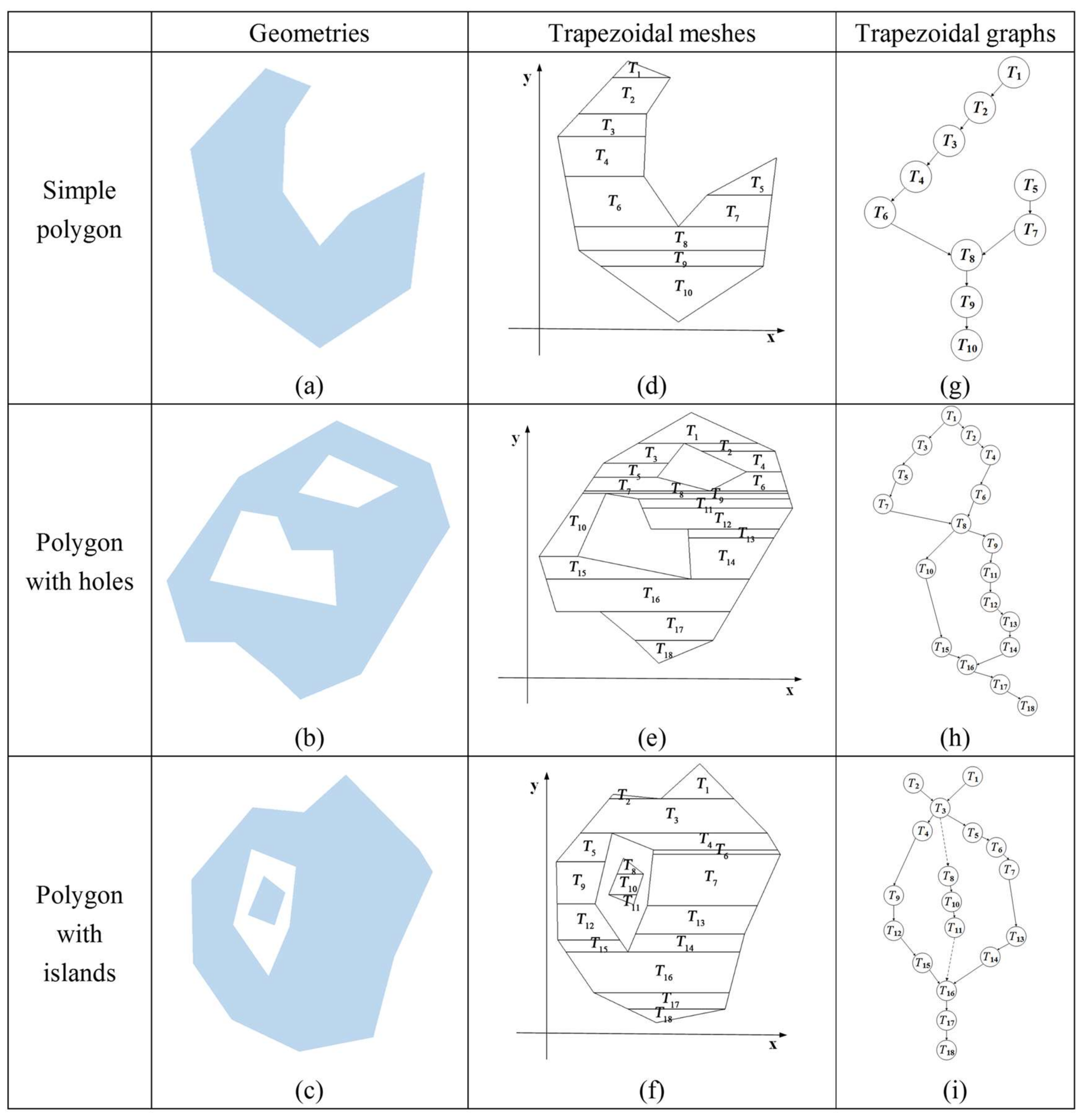
Three forms of polygon are considered for LoD visualization. While polygons have only one exterior boundary, they may contain zero or more interior boundaries, called simple polygons and polygons with holes, respectively. The regions bounded by these interior boundaries may contain additional sets of interior boundaries; these cases are called polygons with islands. Polygons with cut lines, spikes or punctures are not considered in this paper. The considered types of polygons have three forms of topological relationships: islands may not intersect their surrounding boundaries; all boundaries may not self-intersect; and all boundaries must not mutually intersect. These three types of polygons are illustrated in
Figure 1a–c, respectively.
Polygons are tessellated into trapezoidal meshes. For cartographic filling, polygons may need to be tessellated into triangles or trapezoids. To reduce the data rate and increase rendering efficiency, these triangles and trapezoids should be carefully ordered, such as via Hamiltonian triangulations or sequential triangulations in which consecutive triangles share an edge [
32]. Trapezoidation is often performed as a first step of triangulation, and with modern hardware, consecutive trapezoids, i.e., those that share an edge, can achieve similar rendering efficiencies to those of sequential triangulations [
38]. Trapezoidal meshes are chosen to perform polygon LoD visualization. Here, we simplify the trapezoidal meshes of polygons rather than the polygon boundaries (see
Section 5.2 for a more detailed discussion of triangulation and trapezoidation).
Many solutions have been proposed for trapezoidation. One popular solution is the sweep-line algorithm, which can decompose a polygon into trapezoids in any direction [
37]. In this paper, horizontal sweep lines are employed to sweep through each vertex of a polygon from top to bottom. All of the sweep lines are parallel, and they decompose a polygon into a series of vertical strips. A sweep line may cross one or more vertexes, decomposing each strip into one or more trapezoids. Generally, a trapezoid consists of four sides (left, right, bottom and top), of which the top and bottom sides are parallel. In practice, a trapezoid may degenerate into a triangle, as shown in
T1 in
Figure 1d.
Then, the tessellated polygon is organized as a graph in which a trapezoid is modeled as a node and the relationships between two connected trapezoids are modeled as links; the product is called a trapezoidal graph. Various trapezoidal graphs can be created for different polygon instances [
39]. When a node (trapezoid) is connected on one side, either its top or bottom, the node is called a suspended node, as shown by
T1,
T5 and
T10 in
Figure 1d. A convex polygon will be tessellated into a series of trapezoids that are consecutively connected via connecting links. Joined links occur in graphs tessellating a concave polygon, and a division relation occurs when tessellating a polygon with holes. For example, the polygon shown in
Figure 1d is a concave instance that includes several concave points at its exterior boundary. In its corresponding trapezoidal graph, shown in
Figure 1g,
T6 and
T7 join at
T8. The example shown in
Figure 1e is a polygon with two holes. In its corresponding trapezoidal graph, shown in
Figure 1h,
T1 will be divided into
T2 and
T3. If a subgraph starts from a suspended node and ends at a join node or starts from a division node and ends at a join node, then its nodes are consecutively chained, creating a trapezoidal chain. Because the relationships between two connected trapezoids are identical in a trapezoidal chain, trapezoidal chains are isomorphic in terms of their links. Therefore, trapezoids are consecutive, and trapezoidal chains are able to facilitate rendering. For example, when using OpenGL as the rendering engine, a trapezoidal chain can be directly translated into a quad-strip for fast rendering. In addition, because self-intersections and intersections are not allowed, triangles’ (degenerated trapezoid) nodes exist only at the initial or end node of a trapezoidal chain.
Islands are also tessellated into trapezoidal meshes. The trapezoidal mesh of an island will certainly be disjoined from the other trapezoidal meshes. Nevertheless, the trapezoidal meshes of islands are surrounded by other trapezoidal meshes. Thus, pseudo-divided links and pseudo-joined links are derived from divided links and joined links, respectively, to organize these forms of topological relationships (delineated as dashed arrow lines in
Figure 1). The trapezoidal mesh of an island is organized as a subgraph with a pseudo-divided link and a pseudo-joined link. For example, the polygon shown in
Figure 1c is a polygon with an island. In its corresponding trapezoidal graph, shown in
Figure 1i,
T8 and
T3 are connected via a pseudo-divided link, and
T16 and
T11 are connected with a pseudo-joined link.
Trapezoidal graphs encode spatial orders and topological relationships. Because a node corresponds to a trapezoid that specifies a concrete location, nodes are spatially ordered from top to bottom according to the y-coordinates of their top sides and from left to right according to the x-coordinates of their left sides. Specifically, in a trapezoidal graph, a connection link exists for two vertically neighboring trapezoids. A division link also connects two vertically neighboring trapezoids, but the bottom one has at least one sibling. Furthermore, all siblings are mutually separately and ordered via the increasing x-coordinates of their left sides. Similarly, a joined link connects two vertically neighboring trapezoids, but the top one has siblings. All siblings are ordered by their increasing x-coordinates.
The topmost and bottommost nodes are selected as the starting and ending nodes, respectively. If the topmost sweep line crosses more than one vertex, then several top nodes exist and the leftmost node one is chosen as the starting node. Similarly, the rightmost node is chosen as the ending node when several candidates exist. From the starting node, through the aforementioned three types of links (connection, division and joined, including pseudo-divisions and pseudo-joins), all nodes, including the nodes representing islands, can be tracked downward, upward, and to the left and right. From the starting node, trapezoidal chains can also be generated by tracking the connection links.
3.2. Trapezoidal Mesh Simplifications
Given the cartographic simplification rules, a trapezoidal mesh simplification method is introduced in this section. First, a vertex’s weight for preserving the polygon shape is measured. Second, two types of generalization strategies are proposed to generalize the trapezoids. Third, a simplification method is presented that dynamically adapts the trapezoidal meshes according to the zoom level. These operations are discussed in detail below.
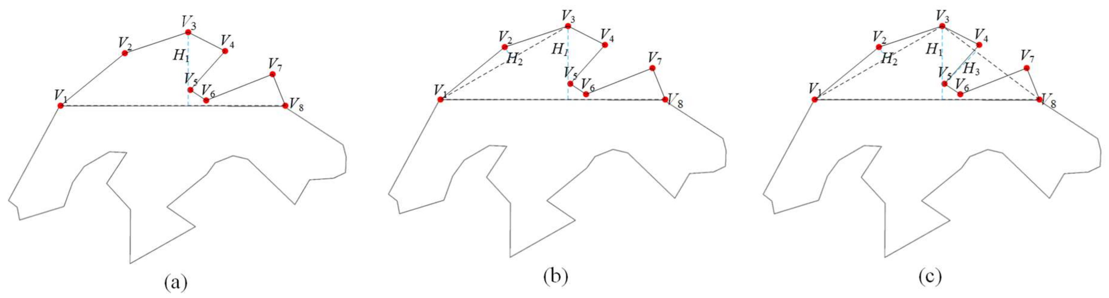
One commonly used cartographic simplification rule is to maintain critical points when simplifying polygons. Many methods have been proposed to determine these critical points [
14,
15], including the widely accepted DP algorithm, which uses a point-to-edge distance to a measure vertex’s weight [
3]. Here, the DP algorithm is chosen to calculate the vertex weights for polygon LoD rendering (see
Section 5.2 for further discussion of the cartographic simplification rules). Similar to the DP-based BLG-tree, all the boundary vertexes are weighted by their point-to-edge distances through binary recursive partitioning. For example, in
Figure 2,
V2,
V3, and
V4 are weighted as
H2,
H1 and
H3, respectively.
Trapezoidal generalizations are then introduced to simplify the trapezoidal meshes according to the vertex weights. Given a zoom level, a threshold value of the point-to-edge distance, denoted as
, can be calculated. When a vertex’s weight is less than the threshold value, then that vertex should be deleted; otherwise, it should be kept to preserve the polygon’s shape [
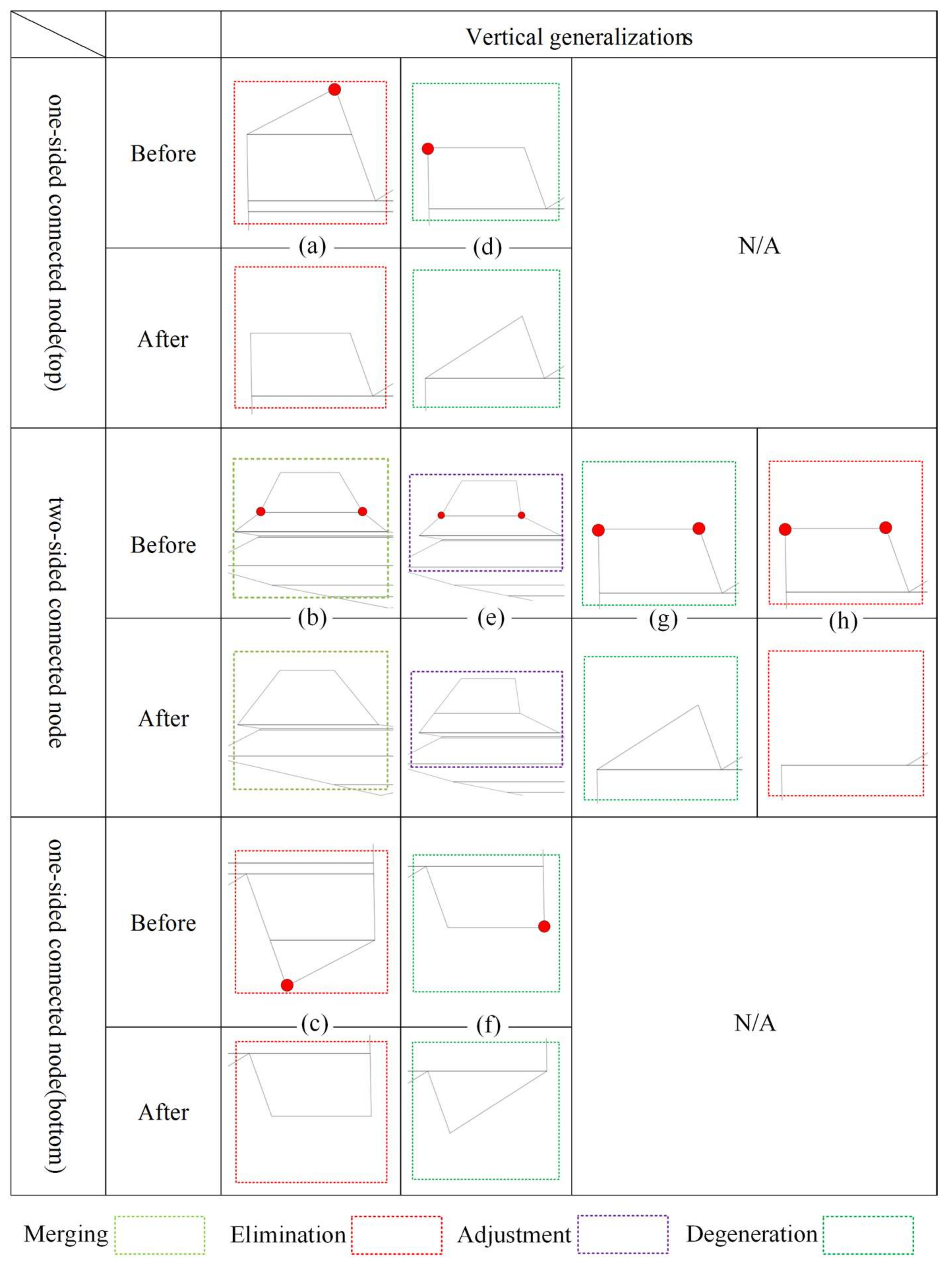
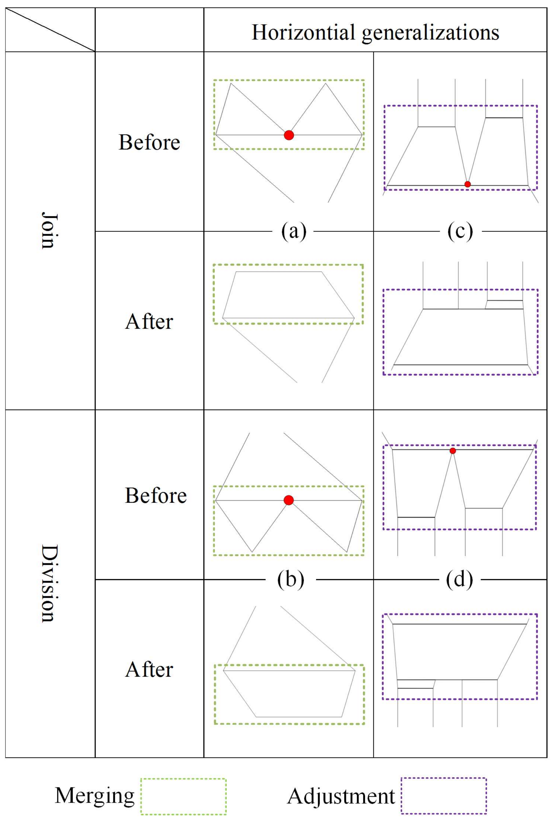
20]. Considering the diversity of polygonal geometries, various trapezoidal and spatial relationships may exist in concrete trapezoidal meshes. Each node may be singly connected with another node above or below itself (i.e., located at the beginning/ending node of a trapezoidal chain). Such nodes are referred to as one-sided connected nodes. Nodes may also be connected with two nodes, one on either side. These nodes are referred to as two-sided connected nodes. For a connection link, the vertically connected trapezoids should be generalized. For a division or a joined link, horizontally connected trapezoids should be generalized.
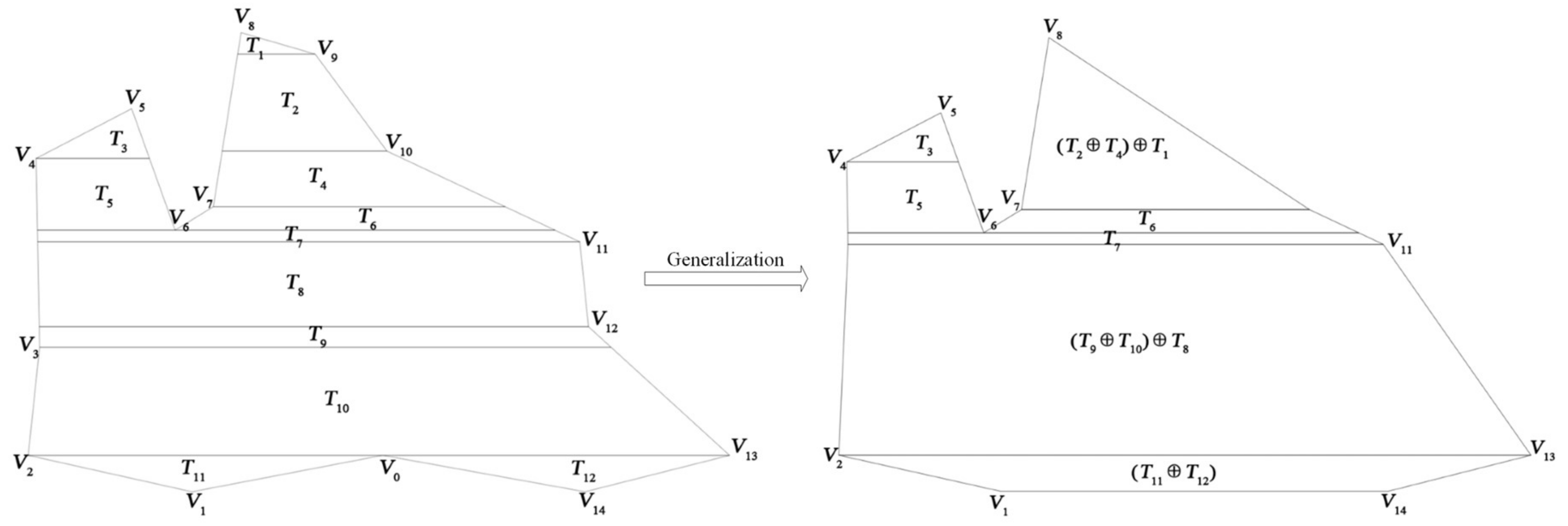
In a vertical generalization, removing a vertex may lead to trapezoid merging, degeneration, elimination or adjustment. When tessellating a polygon into trapezoids, one horizontal side of a trapezoid may cross at least one vertex (its weight is denoted as
w1), which is called a one-vertex horizontal side; it also may cross two vertices (whose weights are denoted as
w1 and
w2, respectively, such that
w1 <
w2), which is called a two-vertex horizontal side. Specifically, four cases exist for vertical merges, distinguishing whether the vertex which needs to be deleted is shared by two trapezoids and whether the horizontal side is a one-vertex horizontal side or a two-vertex horizontal side: (1) if the vertex is shared by two trapezoids and the horizontal side is a one-vertex side (
w1 <
), then the two connected trapezoids will be merged into one. Let the symbol
denote the trapezoid merging operator such that
TiTj stands for the merged result of trapezoids
Ti and
Tj. As shown in
Figure 3, assume that the weight value of
V10 is relatively small. To remove
V10,
T2 and
T4 should be merged. Then,
T2T4 may be further merged with
T1 if
V9 needs to be removed, generating (
T2T4)
T1. (2) If the vertex is shared and the horizontal side is a two-vertex side, then two cases are possible. If the two vertexes that share the horizontal side both need to be deleted (
w1 <
and
w2 <
), as shown in
Figure 4b, then the two connected trapezoids will be merged; if the other vertex needs to be kept (
w1 <
and
w2 >
), as shown in
Figure 4e, then the two connected trapezoids will be adjusted. (3) If the vertex is not shared and it is a one-weight side (
w1 <
), as shown in
Figure 4a, then the trapezoid will be eliminated; (4) If the vertex is not shared and the side is a two-vertex side, as shown in
Figure 4g and
Figure 4h, the trapezoid may collapse into a triangle at the vertex with the smaller weight (
w1 <
and
w2 >
), or be removed (
w1 < and
w2 <
). In total, eight horizontal generalization prototypes are summarized, as shown in
Figure 4.
Similarly, trapezoid merging and adjustment also occur with horizontal generalization. Two horizontally neighboring trapezoids can be involved in horizontal merging, which occurs only at division or joining nodes. The two neighboring trapezoids may be merged into a new trapezoid (see
Figure 5a) or may be adjusted (see
Figure 5c). In total, four merging prototypes are summarized for horizontal generalization, as depicted in
Figure 5.
Because only two trapezoids experience both horizontal and vertical generalization, their nodes and corresponding links can be updated locally without globally rebuilding the graph (the topological changes will be discussed in next section). For example,
Figure 3 shows that merging
T2 and
T4 allows
T2T4 to replace
T2 and
T4, and
T2T4 will correspondingly inherit the connection relationships of
T2 and
T4. That is,
T2T4 are upwardly connected with
T1 and downwardly connected with
T6. Thus, a simplified graph will be generated. The simplified graph represents a simplified trapezoidal mesh and can be translated into consecutive trapezoids for fast rendering.
Based on the generalization prototypes, a trapezoidal mesh simplification method is presented that dynamically chains trapezoidal operators according to their zoom levels. First, a priority stack is introduced. Using binary recursive partitioning, the weighted value of a low level of the partition may be greater than that of a high-level one [
18]. In this paper, the original weight values calculated using the DP algorithm are adjusted as follows to guarantee that the vertex with lower weight value has less importance for preserving the polygon shape:
where
Hi is the weight value for
Vi and is calculated at
levelj though binary recursive partitioning, and
levelj is the parameter for all vertexes that are weighted at
levelj. Sorting the vertexes according to their weights in descending order generates a priority stack. Then, given a zoom level, a threshold weight value can be calculated. By searching the priority stack, those vertexes whose weights are below the threshold are popped from the priority stack. The related nodes and links of popped vertexes are searched, and the relevant trapezoid is then generalized according to the generalization prototypes. By storing the node and corresponding link statuses before and after each generalization operation, trapezoidal merging, degeneration, elimination and adjustment can be undone. After processing all the popped vertexes, the trapezoidal mesh is dynamically simplified. For a simplified trapezoidal mesh, moving to a larger zoom level may cause more vertexes to be popped, causing the trapezoidal mesh to be further simplified. Then, a final version of the tessellated polygons can be generated. If the weight of a popped vertex becomes greater than the threshold value, the vertex is pushed back into the priority stack and its status restored. In this manner, a trapezoidal mesh can be dynamically adapted to a zoom level, and the adapted trapezoidal mesh can be translated into consecutive trapezoids for fast rendering.
3.3. Preserving Topological Consistency
As discussed in
Section 3.1, three forms of topological relationships are considered and should be kept consistent when performing LoD visualization: for an individual boundary, the boundaries should not self-intersect; no two boundaries, exterior or interior, should intersect; and islands should be preserved without intersections. Using the generalization operators discussed in the previous section, when two neighboring trapezoids are generalized, there is a risk of introducing intersections, which violates topological consistency. We simplify the trapezoidal meshes rather than the polygon boundaries. Using this method, topological errors such as self-intersections of a boundary and any intersections between boundaries, including those of islands, are embodied as intersections between trapezoids. Checking for topological correctness is therefore translated into a problem of testing whether the generalized trapezoids intersect with any other trapezoids.
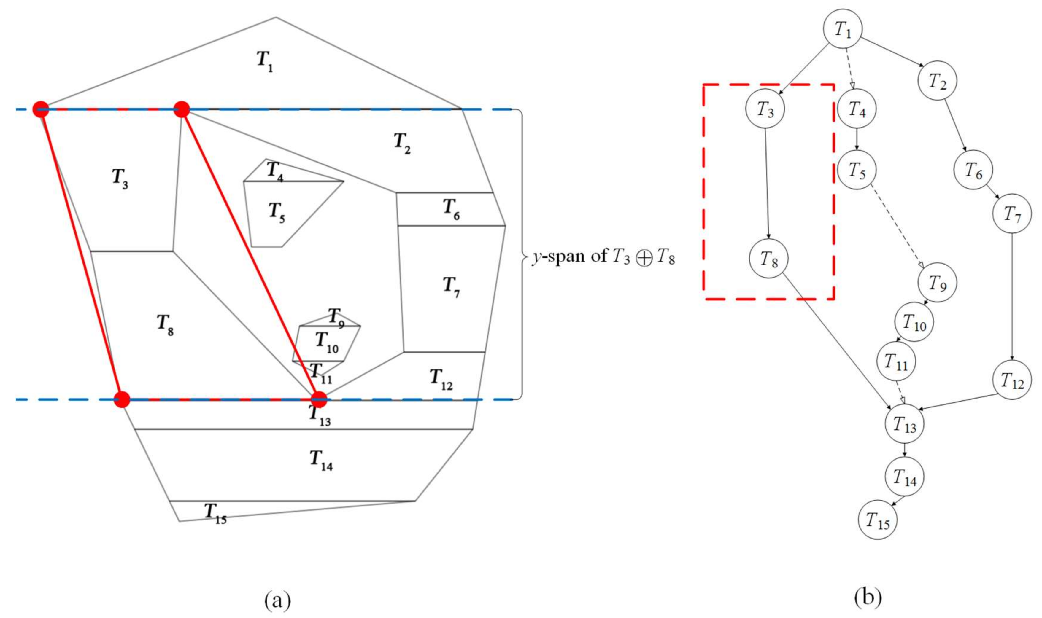
Clearly, topologic errors can be avoided by exhaustively checking whether a generalized trapezoid intersects with any other trapezoid; however, such checks may be too computationally expensive. Therefore, we propose a heuristic testing algorithm to efficiently check for intersections. First, in a trapezoidal mesh, a trapezoid,
Ti cannot intersect with a trapezoid whose projection on the
y-axis does not overlap the
y-span of
Ti. For example, in
Figure 6, assuming
T3 and
T8 will be merged, only trapezoids whose
y-span intersects the
y-span of
T3T8 need to be checked.
Furthermore,
Ti may cover several strips of horizontal trapezoids. In each strip, the trapezoids are ordered by their increasing
x coordinates. The trapezoid closest to
Ti at its right side is denoted as
Ti+1. If
Ti does not intersect with
Ti+1, then
Ti will not intersect with
Tj when
j >
i + 1 and the
y-span of
Tj is within the
y-span of
Ti+1. For example, in
Figure 6, if
T3 does not intersect with
T5, then it will not intersect with
T6. By selecting the closest trapezoids of all the involved strips at both the right and left sides, a minimal surrounding trapezoid set can be found and denoted as
S.
S can be identified via trapezoid tracking. For example, in
Figure 6, the upwardly tracking node of
T3T8 can be identified as the division node
T1. The closest sibling of
T3T8 to the right,
T4, can also be identified. For the downwardly tracking node
T4, the node whose
y-span is within the
y-span of
T3T8 belongs to the minimized surrounding trapezoid set. If the
y-span of
T3T8 is not completely covered, then the downwardly tracking nearest sibling node of
T3T8 to the right (if any) is checked until the
y-span of
T3T8 is either totally covered or all horizontal neighbors to the right side are analyzed. In this manner,
S can be generated without performing a brute-force search of the entire trapezoidal mesh. When a trapezoid belonging to
S is found, it is checked to determine whether it intersects with
T3T8. If the trapezoids intersect, testing ends because an intersection will certainly be introduced. Otherwise, the test continues to the next closest trapezoid. When all items in
S have been visited and no intersection has been reported,
T3T8 is guaranteed to not intersect with any other trapezoid. In this case, the merging operation will not introduce topological inconsistencies.
More generally, a trapezoid may degenerate, be removed, be merged or be adjusted. In any case, the y-span of a generalized trapezoid can be determined, and the minimized surrounding trapezoid set can also be tracked via graph visiting. Benefiting from the structure of a graph in which both order and topology are embedded, heuristic testing of all generalization cases can be performed without a brute-force search. By rejecting generalization operations that introduce trapezoid intersections, topological consistency can be preserved efficiently without exhaustive checks.
6. Conclusions
Polygon LoD visualization is functionally necessary in geo visualization but suffers from low efficiency, especially when visualizing complex polygonal data. Simplification, tessellation and rendering are three major successive phases that are treated as isolated processes in the existing methods, yielding computational and data redundancies that reduce efficiency. In this paper, an efficient method is proposed to facilitate polygon LoD visualization. The contributions of this method are summarized as follows.
Unlike the existing methods, we organize simplification, tessellation and rendering operations into a single mesh generalization process that avoids having to completely re-execute tessellation operations and resend all drawable primitives for rendering. Beyond the supporting techniques such as the sweep line method and the DP algorithm, to the best of our knowledge, this paper is the first to propose the trapezoidal mesh data structure to encode the spatial and topological elements of tessellated polygons, the horizontal and vertical generalizations for rapid trapezoidal mesh simplification, and the heuristic testing algorithm to efficiently preserve topological consistency. In our approach, the simplification and tessellation operations are systematically organized into a single process that avoids computational and data redundancies and helps to mitigate the rate sensitivity.
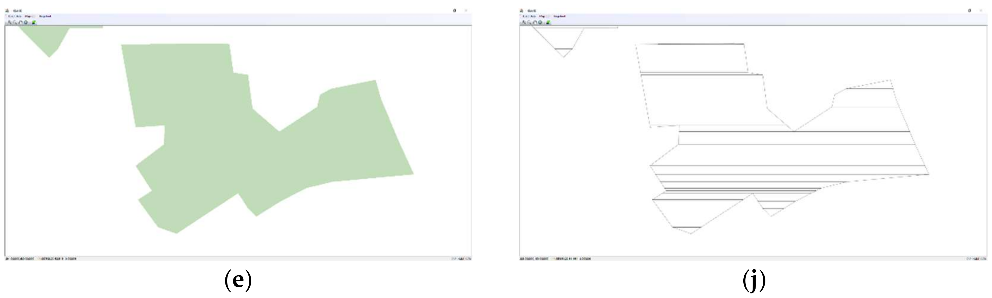
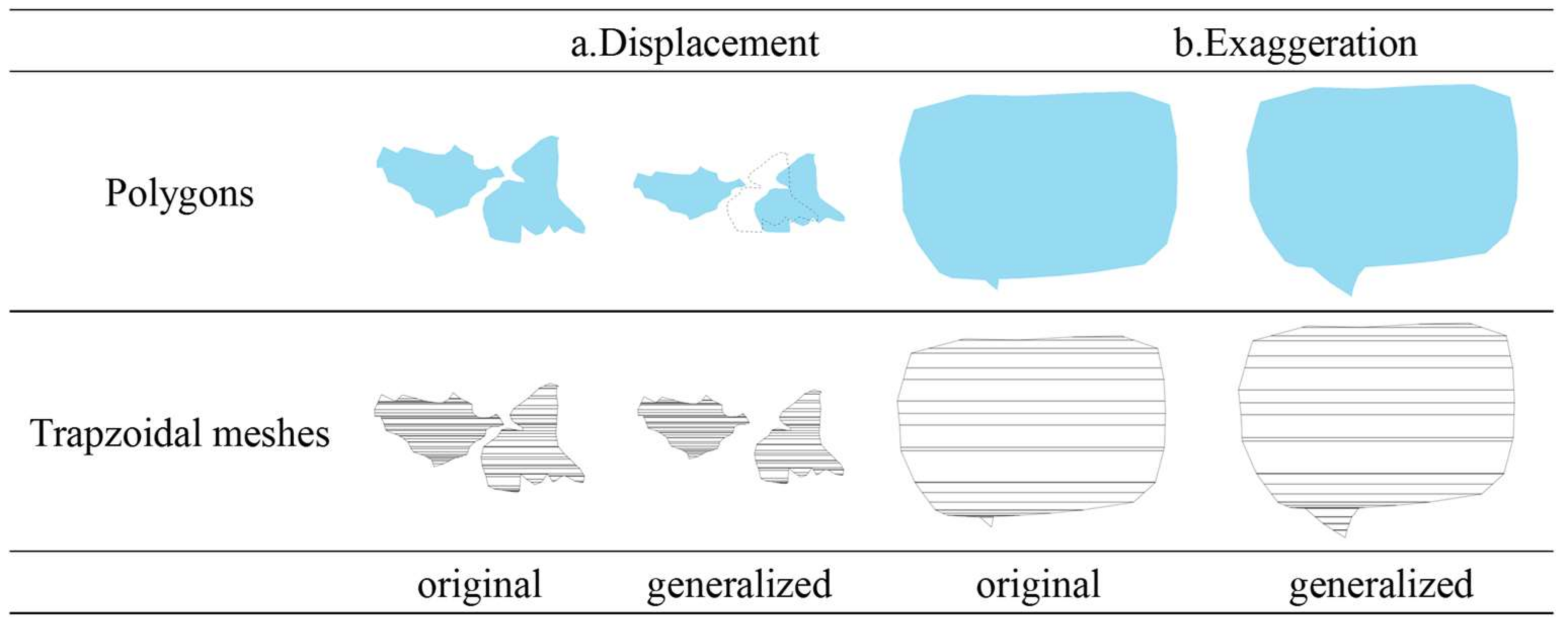
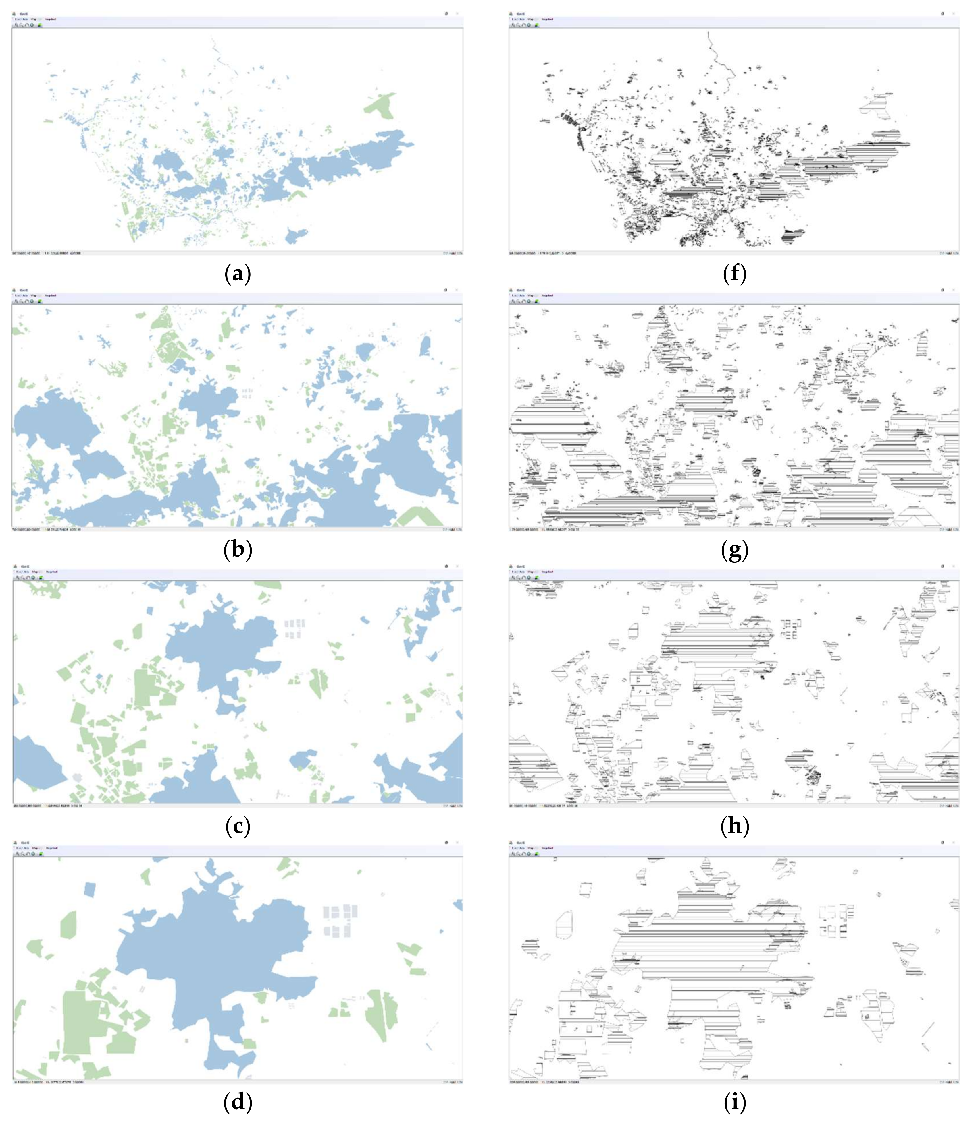
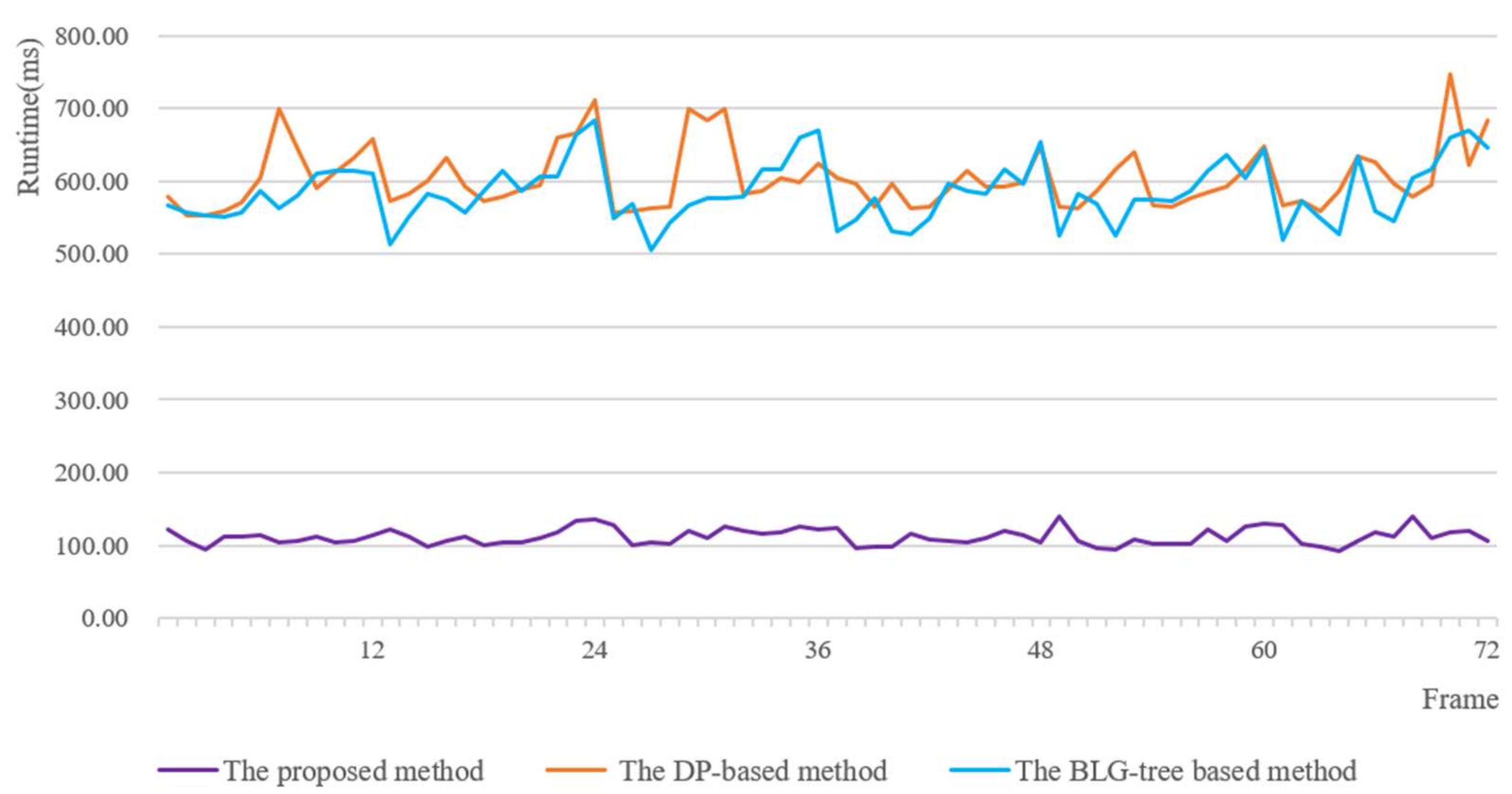
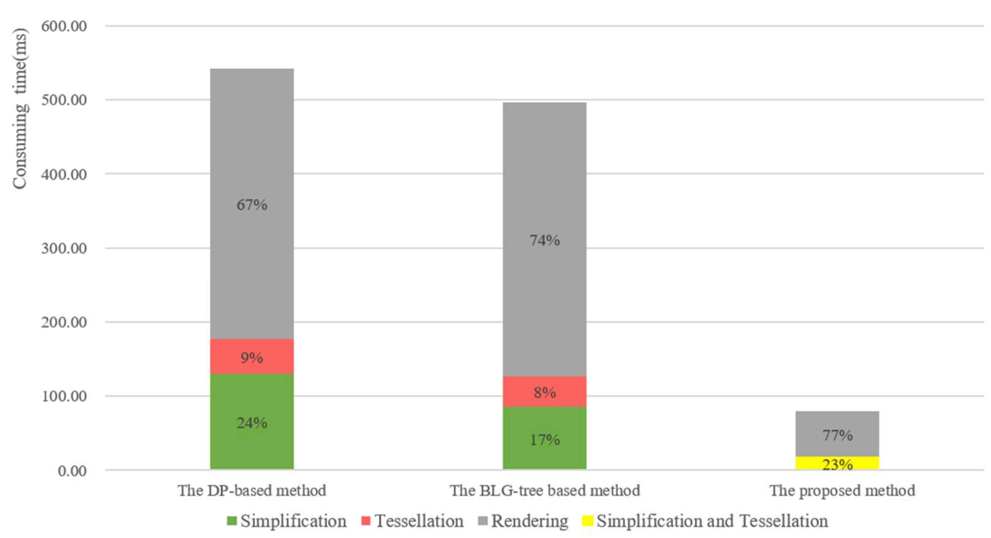
The tests conducted on real world datasets suggest that, compared with the DP-based and BLG-tree-based methods, the proposed method significantly improves the efficiency of polygon LoD visualization. This method can benefit efficiency-sensitive vector mapping applications such as emergency mapping cases in which polygonal data need to be symbolized and simplified in a timely fashion. We implemented and test this algorithm in a desktop environment; however, it could be implemented in a client/server architecture or an embedded system to provide rapid vector mapping responses. Future work will include the consideration of additional criteria for polygon simplification, such as shape preservation, and additional operators to support more complex cartographic generalizations such as displacement and exaggeration. In addition, while trapezoids are generalized individually in this paper, batch generalization will also be addressed in future work. Extending this method to support polygonal maps and even general maps also requires future work.

 ,
, 