Abstract
Transportation is generally perceived as a catalyst for economic development. This has been highlighted in previous studies. However, less attention has been paid to examine the relationship between economy and transport demand by exploring spatially cross-sectional data, especially for countries with significant regional economic imbalance, like China. In this article, we assess the economic influence of intercity multimodal transport demand at the prefecture level in China. Spatial autoregressive regression models are used to examine the impact of transport demand on economy by deep analysis of transport modes (land, air, and water) and regions (eastern, central, and western). Through contrasting results from spatial lag model and spatial error model with those from the ordinary least square, this study finds that the estimation results can become more accurate by controlling for spatial autocorrelation, especially at the national level. Through rigorous analysis it is identified that except for water passenger traffic, all other intercity transport demand significantly contribute to a city’s economic development level in gross domestic product. In particular, air transport demands distribute more evenly and are estimated with the highest beta coefficients at both national and regional levels. In addition, the beta coefficients for land, air and water transportation are estimated with different magnitudes and significances at the national and regional levels. This study contributes to the ongoing discussion on the relationship between intercity multimodal transport demand and economic development level. Findings from this paper provide planning makers with valid and efficient strategies to better develop the economy by leveraging the special “⊣” cluster pattern of economic development and the benefits of air transportation.
1. Introduction
Transportation is widely acknowledged as an important catalyst for economic development, at the regional, national, as well as international level [1,2,3,4]. Transportation provides a vital link in the supply chain of passengers and goods. It enables the market to access to the resultant products [1,5]. In this perspective, it is obvious from a theoretical standpoint that there should be a linkage between transport activity and economy [6].
A number of studies have explored the economic impacts of transport infrastructure investment (e.g., [7,8,9,10,11]), but less attention has been paid to study the association of economy with transport demand [12]. The existing literature highlighted the causal relationship between transportation and economy growth by investigating time series data (e.g., [13,14,15]), whilst less attention has been paid to the association of economy with transport demand by looking into the spatially cross-sectional data. Relatively few studies conducted to explore how the transportation-economy relationship depends on spatial autocorrelation, regional imbalance or intercity transport modes, especially for the rapid and unbalanced development contexts, such as China.
Therefore, researchers need to provide policy-makers with precise and sufficient information to eliminate the relationship between economy and transportation. This study seeks to make up this gap by providing a comprehensive description of spatial transportation-economy relationship through investigating the intercity multimodal transportation data. By examining and comparing passenger traffic and freight volume of land, air, and water independently, the spatial economic impacts of intercity multimodal transportation will be analyzed explicitly. The scope of this study is on China, using prefecture-level cities’ data rather than national/provincial data used in many previous studies [16,17,18,19]. As China has long executed a biased development policy, the transportation and economic development have continuously experienced cross-regional inequality. This case provides a rare perspective to investigate the influence of spatial autocorrelation on the transportation-economy relationship. In addition, using prefecture-level data and spatial autoregressive model, this study will provide more accurate findings for policy-makers.
The remainder of the paper is organized as follows: Section 2 reviews the related literature on the topic and provides a background for this research. Section 3 introduces the study context and data source. Analytical methods are presented in Section 4. Section 5 presents the analysis results. Section 6 discusses the findings, concludes the paper, and provides potential directions for future research.
2. Literature Review
The relationship between transportation and economy has become a very critical topic, especially in developing countries [20]. In less-developed countries, the transport activity generally acts as an important complement to other conditions, whilst in developed countries, the role of transportation in stimulating economic growth is not on its own or straightforward, as it can differ among regions affected by the presence or absence of other drivers of economic growth [21]. While it is hard to generalize the potential economic impacts of transport activity, some empirical studies have found a strong association between transportation and economy, especially based upon time series data exploration [22,23].
Examining a sample of thirty-three countries at different stages of development, Bennathan et al. [24] found a strong relationship between freight transportation and GDP. Additionally, the elasticity of road freight demand with regard to GDP for developing countries was 1.25 times the counterpart of the high-income countries. Using annual time series data of 1970–1995 from India, Kulshreshtha et al. [25] confirmed a long-run structural co-integrating relationship between railway passenger transport and economy. Yao [26] examined the association between freight transportation and industrial production and input inventory investment. Through rigorous analysis, it was confirmed a significant feedback effect upon these entities.
Laplace and Latgé-Roucolle [14] examined the relationship between the economic development and the air traffic in four ASEAN countries including Lao PDR, Myanmar, the Philippines and Vietnam. Their findings pointed out that GDP was very sensible to air traffic growth, especially in the regions which owns only one international airport. Marazzo et al. [15] and Hu et al. [13] explored the relationship between economic growth and air passenger traffic in Brazil and China, respectively. Both studies revealed the significance of air transport in economy development.
However, not all the previous studies found a significant impact of transport activity on economy. For instance, by analyzing data from Brazil throughout the 1966 to 2006 period, Fernandes and Pacheco [27] found that air transportation was affected significantly by economic growth, while the impact of air transport on economic growth was insignificant. Using the panel data of 42 years from South Asia, Hakim and Merkert [12] found the similar result as Fernandes and Pacheco [27].
In addition, most of the existing studies examined the panel data by adopting Granger causal framework rather than exploring cross-sectional data. Granger causality analysis is powerful in examining whether one time series is useful in forecasting another [28], but is less powerful to conduct the cross-sectional analysis horizontally [29]. In addition, most of the previous studies highlighted the temporal correlation of independent variables but neglected the spatial autoregressive effects. From the spatial perspective, the economic performance of an observation not only depends on itself contributors, but may also depend on the contribution of on the neighboring units. Thus, in econometric analysis, it is important to control for spatial autocorrelation especially for countries/regions with regional inequality.
This study seeks to fill in some of the research gaps and shed light on the association of economy with intercity multimodal transportation. Spatial autoregressive regression is used to examine how the economic influence of transportation can become volatile depending on intercity transportation modes and different regions. By exploring prefecture level data from China, findings from this study can provide researchers with knowledge about the relationship between intercity multimodal transportation and economic development level, as well as potential strategies for the regionally-balanceable development.
3. Study Context and Data Source
3.1. Study Context: Regional Inequality in China
Following the reform and open trade policy enacted in 1978, China has experienced remarkable economic development [30]. However, spatial concentration and inequality have also become more severe since then [31,32]. In addition, since China is characterized by regional differentials, spatial inequalities not only exist across regions and provinces, but are also even more evident across cities [33,34]. The growing spatial inequality has drawn increasing scholarly interest and social concern, but sources of spatial inequality in China are still under-studied [35]. Transportation related variables tend to be at play in aggravating the regional inequality [17,18], but little is known about how the economic development impacts of transportation vary depending on regions or intercity transport modes.
Figure 1 illustrates the spatial density distributions of GDP and intercity multimodal transport demand. As can be seen, except for air transportation, the spatial distributions of other economic variables show a classic concentration pattern, with developed cities clustering along the eastern coastal area, the Yangtze River Belt, and the Pearl River Belt, which present the “” shape. The similar spatial distribution of transportation and economy indicates that there may exist a relationship between them. With the aggravation in regional inequality and the advancement of spatial econometric models, it is necessary to examine the hypothesis and discuss the results.
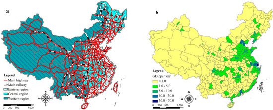
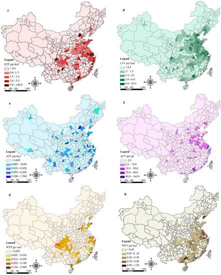
Figure 1.
(a) Three regions and main land transport network in China; density of (b) GDP; (c) land passenger traffic; (d) land freight volume; (e) air passenger traffic; (f) air freight volume; (g) water passenger traffic and (h) water freight volumes.
The Moran’s I tests for the variables are shown in Table 1. The test results confirm that there is less than 1% likelihood that the clustered patterns of GDP, population, and foreign direct investment, land and water transportation could be the result of random chance, while the spatial pattern of air transportation is neither clustered nor dispersed. The tests highlight the potential spatial autocorrelation of many economic related variables in China. Thus, it is necessary to account for the interactions between them to better investigating the relationship between economy and transportation at both national and regional levels.

Table 1.
Moran’s I test of the variables in China.
3.2. Data Source
This study takes prefecture-level cities as the study objects. There are more than 330 prefecture-level cities in China. Due to data availability, this study analyzed the data from 277 cities (including four municipalities of Beijing, Shanghai, Tianjin, and Chongqing). The dependent variable examined in this study is the gross domestic product (GDP), an important factor that reflects the economic development levels of cities. For the independent variables, both passenger traffic and freight volume of each transportation mode of land, air, and water are included and investigated. One-year cumulative GDP and transportation data of 2012 were collected from China City Statistical Yearbook. Since 2013, the National Bureau of Statistics of China (NBSC) required the local transport agencies to use a new statistic method to report the transport related data to NBSC. Whilst some local transport agencies used the new statistic method following NBSC’s requires, some others did not. As Figure 2 shows, the multi-standard caused confusion to some extent and reduced the accuracy of data especially for land passenger traffic in the following years. To keep consistent in statistic method for each city and improve the data accuracy, we used 2012 data in this study. In addition to the variables that reflect transport demand, two important independent variables—population and foreign direct investment (FDI) that may significantly affect GDP are examined. Due to data availability from China City Statistical Yearbook, other independent variables such as education and knowledge economy that may also affect GDP were not included. In addition, as the municipalities generally enjoy more specific development policies than other cities, one dummy variable of municipality (1) or not (0) is included for examination. Table 2 shows the variable statistics.
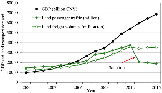
Figure 2.
GDP and land transportation at the national level in China, 2000–2015. (Source, NBSC <www.stats.gov.cn>).
Table 2.
Variable statistics.
Table 3 reports the estimation coefficients of correlation matrix. The results show a strong correlation between GDP and the independent variables. The weakest correlation is observed between GDP and water passenger traffic with estimated Pearson coefficient of only 0.202. The correlation matrix also shows a strong correlation between some independent variables. Especially, the Pearson coefficients between total and land passenger traffic, total, and land freight volume, as well as between air passenger traffic and air freight volume, are much higher than the rule-of-thumb of co-linearity threshold of 0.7 [36,37]. Thus, the pair variables mentioned above should not be included into the models simultaneously. Indeed, we intend to examine the association of GDP with the total or each transportation mode separately. Thus, Table 2 is mainly used to highlight the positive relationship between the GDP and the independent variables.
Table 3.
Correlation matrix.
4. Statistical Models
As mentioned above, the GDP of a city not only depends on the independent variables, but also on the economic development of the surrounding cities. In other words, there may exist significantly spatial interaction between the dependent variables. To examine this hypothesis, two main statistical models, i.e., non-spatial model and spatial autoregressive (SAR) model, are performed in this study.
4.1. Non-Spatial Model
An initial non-spatial model of OLS without controlling for spatial autocorrelation is developed to examine the impacts of population (POP), FDI and the city character (i.e., (municipality or not (MUN)) on GDP the. Accordingly, the basic OLS model is given as:
where denotes the dependent variable of gross domestic product. represents population. is the foreign direct investment. represents the dummy indicator of whether a city is municipality or not. denotes the independent variables of intercity multimodal transportation of total, land, air or water. , , , , and are the constants to be estimated. represents the error term.
4.2. Spatial Autoregressive (SAR) Model
A main debate on the non-spatial model is its ability in accounting for the spatial correlation among observations. With the advancement of spatial econometric models, it is both necessary and possible to perform spatial regression models to control for the interactions of cross-sectional units. Various spatial autoregressive (SAR) models have been introduced and further developed by Whittle’s [38], Anselin [39], Getis and Ord [40], Anselin [41], Fingleton [42], etc. Depending on where the spatial interactions occur, two classic spatial models are considered in this paper: (1) SAR lag model (SLM); and (2) SAR error model (SEM). The SLM accounts for the spatial autocorrelation in the dependent variables and takes the form as:
where denotes the spatially-lagged GDP for spatial weights matrix . is the coefficient to be estimated. The row-standardized weight matrix is used to characterize the spatial weights matrix used here is (refer to Anselin [41] for details).
The SEM accounts for the spatial autocorrelation among residuals. It contains a spatial error term and examines the impact of omitted variables on observations [43]. The SEM is expressed by:
With:
where is the autoregressive coefficient to be estimated, and denotes the error term.
In the SLM model, if is significant, it indicates that there is spatial interaction among the dependent variables. Similarly, when is significant, it indicates significant spatial correlation that occurs at the error component [44].
State of the art of SLM and SEM is far more complex than the usage of GIS and GeoDa [45]. Developed by Anselin [41], this paper adopts a three-step spatial data analysis approach to facilitate the usage of SAR model. First, establish the initial OLS model and test the validation of the model. Second, perform the initial OLS model and obtain the spatial autocorrelation statistics such as Moran’s I (error), Lagrange multiplier (lag), and four other test statistics. Third, based on the statistics, we estimate SLM and SEM, and examine and discuss the results.
5. Results
Table 4 represents the results of five non-spatial models that estimate the impacts of independent variables on GDP at the national level. The results of Model 1 indicate that both passenger traffic and freight volume are significantly and positively related to GDP. With estimated coefficients of 0.060 and 0.881, respectively, both population and FDI especially the FDI are strongly associated with the economic development. This is consistent with the previous studies [46,47]. The estimated coefficients for total passenger traffic and total freight volume are 0.308 and 0.469, respectively, both of which are significant at the 1% level. In addition, estimated with the positive coefficient of 257.04, the dummy variable of municipality or not is highly related to GDP. This result indicates that there are other factors that affect the economic development level. Such as the municipality of Shanghai, it is clear that the current levels of economic development and transportation demand are very high. However, other determinants that are not examined in this study, such as development strategies and knowledge economy may also be at play. The readers are referred to existing studies for more details (e.g., [48,49,50,51]). Models 2–5 examine the relationship between GDP and intercity transport demand by modes of land, air and water. Table 3 shows the correlation matrix which indicates that the degree of co-linearity between air passenger traffic and freight volume is higher than the threshold of 0.7. Thus, the APT-GDP and AFV-GDP relationship is estimated separately, as models 3 and 4 show. The estimation results show that only water passenger is not significantly associated with GDP at the national level. In all estimated models, the dummy variable denoting a city is municipality or not is significant and contributes to GDP positively. The estimated coefficients for land passenger traffic and freight volume are 0.54 and 0.65, respectively, and both are significant at the 1% level. The highest estimated coefficients are obtained for the air transportation, indicating air transportation have the strongest potentials in improving the economic development level. However, this may also be due to the fact that air transportation in China only accounts for a very small percentage of the total transportation. For instance, the air passenger traffic of China at the end of 2012 was 529.9 million, accounting for only 1.28% of the total passenger traffic [52]. These initial findings indicate that air transportation is an important indicator for the level of economic development of a city, and also have a strong growth potential in China in the future.
Table 4.
Non-spatial estimation results.
Table 5 shows the modeling results of SLM and SEM for the association of GDP with transport demand at the national level. As can be seen, only in the SLM Model 1 is not statistically significant. After excluding population and FDI, significantly spatial autocorrelation is at play in models 2–5. In recognition of the significance of spatial autocorrelation, the estimators from the SLM or SEM can characterize the association of economy with intercity multimodal transport demand more accurately. For the case of the dependent variable (GDP) with spatial autocorrelation and independent variable without spatial autocorrelation, the robustness of SLM/SEM models, especially the SLM models are better than that of OLS as verified by the Breusch-Pagan test result. For instance, the Breusch-Pagan test for OLS in Model 3 in Table 3 is 9.73, compared to the counterparts of 18.24 for SLM and 14.84 for SEM, respectively. In addition, compared to the non-spatial models, the spatial model fitness improved. For instance, the for land transportation is 0.665 in the initial OLS model in Table 4, but increases to 0.706 in the SEM model in Table 5.
Table 5.
SLM/SEM estimation results at the national level.
The beta coefficients of independent variables are relatively stable. The marginal coefficients for total passenger traffic and freight volume range between 0.308 and 0.311, 0.464 and 0.469, respectively. Only water passenger traffic is statistically insignificant in estimating a city’s GDP, even after controlling for spatial autocorrelation. Additionally, air transportation of APT and AFV are again estimated with the highest marginal coefficients in both SLM and SEM.
Table 6, Table 7 and Table 8 show the SLM and SEM modeling results for the eastern, central, and western regions, respectively (please refer to Appendix A for the non-spatial modeling results for the three regions). We firstly noted that the spatial autocorrelation between GDP, as well as between hidden independent variables become less significant or even absent at the regional level. For instance, the estimated of W_GDP for land and water transportation are significant at the 0.01 level in models 2 and 5, respectively, in Table 5, but become statistically insignificant in Table 6.
Table 6.
SLM/SEM estimation results for the eastern region.
Table 7.
SLM/SEM estimation results for the central region.
Table 8.
SLM/SEM estimation results for the western region.
For the eastern region, the estimated beta coefficients for land passenger traffic and freight volume from SLM are 0.602 and 1.238, respectively, are larger than the counterparts of 0.507 and 0.660 from the national models. This finding indicates that the marginal effect of land transport demand is much stronger in the eastern region. However, the marginal impact of water freight volume on GDP is weaker, as its estimated coefficient decreases from 2.143 in the national model to 1.758 in eastern model. In the eastern region, a city’s GDP tends to be more significantly depended on the intercity multimodal transportation, as the model fitness of R2 for the eastern region are higher than those in the national model.
Table 7 shows that in the central region of China, the impact of total freight volume on GDP is insignificant in both SLM and SEM. Even without controlling for the influence of population and FDI, the relationship between GDP and land freight volume is statistically insignificant in the SLM model. However, the association of GDP with land freight volume is significant at the 0.05 level in the SEM model. While the total/land freight volume becomes less significant, the association of GDP with total/land passenger traffic becomes stronger. In addition, the marginal effects of air transportation and water freight volume on the GDP in the central region also become stronger. For instance, the estimated coefficients of air passenger traffic and water freight volume in the SLM models for the central region are 69.555 and 2.621, respectively, compared to the counterparts of 21.249 and 2.143 in the national models. These results indicate that in the central region, air and water transportation are more strongly associated with GDP. From the geographic point of view, these results are reasonable as many cities with higher GDP such as Wuhan, Changsha, Hefei, Nanchang, etc., are located along the Yangtze River, with more water cargos than other cities in the central region.
Table 8 presents the SLM and SEM estimation results for the western region. As can be seen, except for water transportation, the other intercity transportation modes including land and air transportation are all statistically significant in the estimated models. In particular, the total freight volume and LFV play a stronger role in a city’s GDP in the western region compared to their impact at the national level. Air cargo significantly associates with GDP, and its impact on GDP in the western region is stronger than that in the national models. However, both water passenger traffic and freight volume are absent in the estimated model in the western region. In addition, the dummy variable of municipality or not is significant but the estimated coefficient is negative in explaining GDP in Model 1. This requires careful interpretation. In the western region of China, Chongqing is the only municipality. With a population of 29.45 million, its GDP in 2012 was 1141 billion [52]. Compared to the western cities of Chengdu (with population of 14.17 million and GDP of 814 billion in) and Xi’an (population of 8.55 million and GDP of 437 billion) in the same year, the municipality of Chongqing has no advantage in GDP per capita. Thus, the dummy variable of municipality (Chongqing) is estimated with negative coefficient especially by including population for estimation.
At the national level as well as for the three regions of eastern, central, and western, both population and FDI are significantly associated with GDP. In particular, the population is estimated with the highest coefficient of 0.147 (SLM estimation results) in the eastern region, while FDI has the strongest marginal effect (estimated with beta coefficient of 2.950 in the SLM) on GDP in the central region. While we did not focus on the economic impact of FDI, the results from the current study shed light on the association of GDP with FDI by controlling for spatial autocorrelation.
6. Discussion and Conclusions
This study seeks to analyze the relationship between GDP and intercity multimodal transport demand at both national and regional levels in China. Data from 277 prefecture-level cities (including four municipalities) are used to explore the relationship. Three main intercity transportation modes are examined including land transportation, air transportation, and water transportation. The 277 cities is categorized into three regions according to their geographical locations: the eastern, the central, and Western China. Spatial autoregressive regression is performed to examine the relationship. The estimation result is also compared with those from the ordinary least square. Both regression analysis and contrastive analysis are conducted to examine how economic effects of intercity transport demand vary depending on modes, regions, and spatial interaction.
Findings from this study indicate that at the nation level in China, many economic related variables demonstrate significantly spatial cluster pattern. Most of the cities with high GDP, intercity transportation, and population and FDI are densely located along the coastal area and the Yangtze River belt. There are also some exceptions, such as the air transportation, which generally distribute neither clustered nor dispersed. However, the economic cluster pattern is a visible sign of regional disparity and is considered to be an unsustainable and inefficient economic development strategy [53,54]. The “” cluster pattern presents a potential by utilizing the spatial spillover effect of the cities with higher economic or transportation levels, but how to implement this strategy in China with vast territory is still a great challenge.
Based on the results from this study, two strategies could be recommended to mitigate the regional disparity. The first strategy relates to the spillover effect of megacities with high level of economy and transportation. Most of megacities at this stage are mainly distributed in the three economic circles located in the Eastern China, such as Shanghai in the Yangtze River Delta, Shenzhen and Guangzhou in the Pearl River Delta, and Beijing and Tianjin in the Bohai Economic Rim. Whilst cities in the both central and western region such as Wuhan, Changsha, Chongqing and Chengdu have also enjoyed rapid development in recent years, there is still a large gap in the economic development level between the megacities in the eastern region and central/western region. As the megacities tend to play a significant role in promoting development of economy, it is necessary to accelerate the development of core cities to boost the development of surrounding regions.
On the other hand, the modeling results reveal that the air transportation is estimated with the highest coefficients at both national and regional levels. Some previous studies also suggested that growth in GDP was very sensible to growth in air traffic for time dimension [13,14], findings from this study further indicate that air transportation is strongly associated with GDP across cities in China. Indeed, results from this study identified that only the intercity air transportation (in terms of both air passenger traffic and freight volume) have noticeable influence on GDP at the national level and in all the three regions. Additionally, unlike land and water transportation, air transportation does not show a clustered pattern at the national level, which tends to be a more sustainable and efficient development pattern. Further, considering the fact that air transportation still accounts for a very small percentage of the total transportation in China, it is possible and necessary to promote the air transportation development to enhance the development of GDP.
At the regional level, the spatial autocorrelation becomes less significant or even absent. This is reasonable since cluster pattern generally becomes less obvious at a smaller geographical scale. The magnitudes of the estimated coefficients indicate that in the eastern region, the impact of water transportation on GDP is not significant, while the land transportation tend to be more strongly associated with GDP. However, for the central region, the estimation results are just opposite to those for the eastern region. These findings indicate that geography is an important factor to account for the relationship between GDP and intercity transport demand. In addition, air transportation plays the strongest role in affecting GDP in the central region.
By controlling for spatial autocorrelation, this paper has established a sound foundation for the association of GDP with intercity multimodal transport demand at both national and regional levels in China. Considering the gaps of economic development in different regions of China keeps expanding, an efficient development strategies is needed to reduce the spatial inequalities at both national and regional levels. Our research has important implications for transport planning and development in this context. First, transport planning needs to reconsider the spatial inequality of transport development in China. Except for air transportation, both land and water transportation show a significantly cluster pattern at the national level. In recognition of the contribution of transportation to economy, it is necessary to develop effective transport development strategy in the western and central regions to promote economic development. In addition, only air transportation show a relatively balanced development pattern and are strongly associated with GDP. Thus, findings from this study highlight the potential of promoting the development of air transportation in the vast China to enhance the economic development in China.
This study has a few limitations, which provide potential directions for future research. First, this study focused on the spatial econometric analysis on the association of intercity multimodal transport demand with the levels of GDP at the both national and regional level in China. Future studies may need to explore the panel data to examine the causal link between intercity transportation and economic growth rates. Furthermore, the estimated models neglect the impact of transport development polices as the logistics hub planning at prefectural level is not available. With the advancement of econometric models and data availability, more interesting and new findings of the economic impacts of transportation are expected.
Acknowledgments
The study was funded by the National Science Foundation of China (51608313 and 51508315), and the City and University Integration Program of Zibo (2017ZBXC015). The authors would also want to express their gratitude for the valuable comments and suggestions from three anonymous reviewers.
Author Contributions
J.Z. conceived the study; the manuscript was written by J.Z., J.W., and D.G.; H.Z. analyzed the data; and Z.Y. analyzed the data and revised the manuscript. All authors have read and approved the final manuscript.
Conflicts of Interest
The authors declare no conflict of interest.
Appendix A
Table A1.
Non-spatial model estimation results.
Table A1.
Non-spatial model estimation results.
| Model 1 | Model 2 | Model 3 | Model 4 | Model 5 | ||||||
|---|---|---|---|---|---|---|---|---|---|---|
| Coeffi. | p | Coeffi. | p | Coeffi. | p | Coeffi. | p | Coeffi. | p | |
| Constant | −12.902 | 0.577 | 22.843 | 0.439 | 238.197 | 0.000 | 259.546 | 0.000 | 231.259 | 0.000 |
| (26.911) | (0.075) | (25.700) | (0.195) | (109.772) | (0.000) | (112.420) | (0.000) | (120.792) | (0.000) | |
| [6.630] | [0.499] | [10.592] | [0.169] | [81.188] | [0.000] | [94.267] | [0.000] | [108.750] | [0.000] | |
| POP | 0.155 | 0.002 | / | / | / | / | / | / | / | / |
| (0.077) | (0.043) | / | / | / | / | / | / | / | / | |
| [0.054] | [0.061] | / | / | / | / | / | / | / | / | |
| FDI | 0.606 | 0.000 | / | / | / | / | / | / | / | / |
| (2.951) | (0.000) | / | / | / | / | / | / | / | / | |
| [2.069] | [0.000] | / | / | / | / | / | / | / | / | |
| TPT | 0.418 | 0.000 | / | / | / | / | / | / | / | / |
| (0.456) | (0.002) | / | / | / | / | / | / | / | / | |
| [0.181] | [0.003] | / | / | / | / | / | / | / | / | |
| TFV | 0.588 | 0.000 | / | / | / | / | / | / | / | / |
| (0.000) | (0.999) | / | / | / | / | / | / | / | / | |
| [0.538] | [0.000] | / | / | / | / | / | / | / | / | |
| LPT | / | / | 0.608 | 0.000 | / | / | / | / | / | / |
| / | / | (0.932) | (0.000) | / | / | / | / | / | / | |
| / | / | [0.403] | [0.000] | / | / | / | / | / | / | |
| LFV | / | / | 1.249 | 0.000 | / | / | / | / | / | / |
| / | / | (0.250) | (0.169) | / | / | / | / | / | / | |
| / | / | [0.687] | [0.000] | / | / | / | / | / | / | |
| APT | / | / | / | / | 20.178 | 0.000 | / | / | / | / |
| / | / | / | / | (68.285) | (0.000) | / | / | / | / | |
| / | / | / | / | [18.595] | [0.000] | / | / | / | / | |
| AFV | / | / | / | / | / | / | 8.559 | 0.000 | / | / |
| / | / | / | / | / | / | (82.978) | (0.000) | / | / | |
| / | / | / | / | / | / | [12.594] | [0.000] | / | / | |
| WPT | / | / | / | / | / | / | / | / | 2.029 | 0.825 |
| / | / | / | / | / | / | / | / | (−6.440) | (0.672) | |
| / | / | / | / | / | / | / | / | [−1.982] | [0.820] | |
| WFV | / | / | / | / | / | / | / | / | 1.861 | 0.000 |
| / | / | / | / | / | / | / | / | (2.615) | (0.000) | |
| / | / | / | / | / | / | / | / | [−0.280] | [0.820] | |
| MUN | 433.229 | 0.000 | 940.989 | 0.000 | 522.618 | 0.001 | 604.514 | 0.003 | 1088.708 | 0.000 |
| / | / | / | / | / | / | / | / | / | / | |
| [−226.725] | 0.007 | [−56.600] | [0.492] | [826.776] | [0.000] | [896.867] | [0.000] | [1093.180] | [0.000] | |
| R2 | 0.926 | 0.799 | 0.716 | 0.608 | 0.563 | |||||
| (0.713) | (0.405) | (0.634) | (0.723) | (0.144) | ||||||
| [0.931] | [0.903] | [0.738] | [0.582] | [0.502] | ||||||
| No. of observations | 97 | |||||||||
| (95) | ||||||||||
| [85] | ||||||||||
“/” Indicates this variable is not included into estimation. Note: Estimators for the central are shown in parenthesis. Estimators for the central are shown in brackets. Coefficients with p-value less than 0.1 are shown in bold.
References
- Lee, M.K.; Yoo, S.H. The role of transportation sectors in the Korean national economy: An input-output analysis. Transp. Res. Part A 2016, 93, 13–22. [Google Scholar] [CrossRef]
- Limani, Y. Applied relationship between transport and economy. IFAC-Pap. OnLine 2016, 49, 123–128. [Google Scholar] [CrossRef]
- Saidi, S.; Hammami, S. Modeling the causal linkages between transport, economic growth and environmental degradation for 75 countries. Transp. Res. Part D 2017, 53, 415–427. [Google Scholar] [CrossRef]
- Tsekeris, T. Domestic transport effects on regional export trade in Greece. Res. Transp. Econ. 2017, 61, 2–14. [Google Scholar] [CrossRef]
- Coyle, J.J.; Bardi, E.J.; Cavinato, J.L. Transportation, 3rd ed.; West Publishing Company: Cincinnati, OH, USA, 1990. [Google Scholar]
- Gkritza, K.N.; Vadali, S.R. Special issue on transportation and economic development. Res. Transp. Econ. 2017, 61, 1. [Google Scholar] [CrossRef]
- Chi, J.; Baek, J. Dynamic relationship between air transport demand and economic growth in the United States: A new look. Transp. Policy 2013, 29, 257–260. [Google Scholar] [CrossRef]
- Jiang, X.; He, X.; Zhang, L.; Qin, H.; Shao, F. Multimodal transportation infrastructure investment and regional economic development: A structural equation modeling empirical analysis in China from 1986 to 2011. Transp. Policy 2017, 54, 43–52. [Google Scholar] [CrossRef]
- Laird, J.J.; Venables, A.J. Transport investment and economic performance: A framework for project appraisal. Transp. Policy 2017, 56, 1–11. [Google Scholar] [CrossRef]
- Legaspi, J.; Hensher, D.; Wang, B. Estimating the wider economic benefits of transport investments: The case of the Sydney North West Rail Link project. Case Stud. Transp. Policy 2015, 3, 182–195. [Google Scholar] [CrossRef]
- Song, L.; Geenhuizen, M. Port infrastructure investment and regional economic growth in China: Panel evidence in port regions and provinces. Transp. Policy 2015, 42, 173–179. [Google Scholar] [CrossRef]
- Hakim, M.M.; Merkert, R. The causal relationship between air transport and economic growth: Empirical evidence from South Asia. J. Transp. Geogr. 2016, 56, 120–127. [Google Scholar] [CrossRef]
- Hu, Y.; Xiao, J.; Deng, Y.; Xiao, Y.; Wang, S. Domestic air passenger traffic and economic growth in China: Evidence from heterogeneous panel models. J. Air Transp. Manag. 2015, 42, 95–100. [Google Scholar] [CrossRef]
- Laplace, I.; Latgé-Roucolle, C. Deregulation of the ASEAN air Transport Market: Measure of Impacts of Airport Activities on Local Economies. Transp. Res. Procedia 2016, 14, 3721–3730. [Google Scholar] [CrossRef]
- Marazzo, M.; Scherre, R.; Fernandes, E. Air transport demand and economic growth in Brazil: A time series analysis. Transp. Res. Part E 2010, 46, 261–269. [Google Scholar] [CrossRef]
- Chen, Z.; Xue, J.; Rose, A.Z.; Haynes, K.E. The impact of high-speed rail investment on economic and environmental change in China: A dynamic CGE analysis. Transp. Res. Part A 2016, 92, 232–245. [Google Scholar] [CrossRef]
- Demurger, S. Infrastructure and economic growth: An explanation for regional disparities in china? J. Comp. Econ. 2001, 29, 95–117. [Google Scholar] [CrossRef]
- Hong, J.J.; Chu, Z.F.; Wang, Q. Transport infrastructure and regional economic growth: Evidence from China. Transportation 2011, 38, 737–752. [Google Scholar] [CrossRef]
- Yu, N.N.; Jong, M.D.; Storm, S.; Mi, J.N. The growth impact of transport infrastructure investment: A regional analysis for China (1978–2008). Policy Soc. 2012, 31, 25–38. [Google Scholar] [CrossRef]
- Banister, D.; Berechman, Y. Transport investment and the promotion of economic growth. J. Transp. Geogr. 2001, 9, 209–218. [Google Scholar] [CrossRef]
- Meersman, H.; Nazemzadeh, M. The contribution of transport infrastructure to economic activity: The case of Belgium. Case Stud. Transp. Policy 2017, 5, 316–324. [Google Scholar] [CrossRef]
- Beyzatlar, M.A.; Karacal, M.; Yetkiner, H. Granger-causality between transportation and GDP: A panel data approach. Transp. Res. Part A 2014, 63, 43–55. [Google Scholar] [CrossRef]
- Zhao, J.; Yu, Y.; Wang, X.; Kan, X. Economic impacts of accessibility gains: Case study of the Yangtze River Delta. Habitat Int. 2017, 66, 65–75. [Google Scholar] [CrossRef]
- Bennathan, E.; Fraser, J.; Thompson, L.S. What Determines Demand for Freight Transport? Working Paper No. WPS 998; Infrastructure and Urban Development Department; World Bank: Washington, DC, USA, 1992. [Google Scholar]
- Kulshreshtha, M.; Nag, B.; Kulshrestha, M. A multivariate cointegrating vector auto regressive model of freight transport demand: Evidence from Indian railways. Transp. Res. Part A 2001, 35, 29–45. [Google Scholar] [CrossRef]
- Yao, V.W. The causal linkages between freight transport and economic fluctuations. Int. J. Transp. Econ. 2005, 32, 143–159. [Google Scholar]
- Fernandes, E.; Pacheco, R.R. The causal relationship between GDP and domestic air passenger traffic in Brazil. Transp. Plan. Technol. 2010, 33, 569–581. [Google Scholar] [CrossRef]
- Granger, C.W.J. Investigating causal relations by econometric models and cross spectral methods. Econometrica 1969, 37, 424–438. [Google Scholar] [CrossRef]
- Mariusz, M. A review of the Granger-causality fallacy. J. Philos. Econ. 2015, 8, 86–105. [Google Scholar]
- Tian, X.; Zhang, X.; Zhou, Y.; Yu, X. Regional income inequality in China revisited: A perspective from club convergence. Econ. Modell. 2016, 56, 50–58. [Google Scholar] [CrossRef]
- Pedroni, P.; Yao, J.Y. Regional income divergence in China. J. Asian Econ. 2006, 17, 294–315. [Google Scholar] [CrossRef]
- Zhang, Q.; Zou, H. Regional inequality in contemporary China. Ann. Econ. Financ. 2012, 13, 113–137. [Google Scholar]
- He, S.; Bayrak, M.M.; Lin, H. A comparative analysis of multi-scalar regional inequality in China. Geoforum 2017, 78, 1–11. [Google Scholar] [CrossRef]
- Li, Y.; Wei, Y.H.D. The spatial-temporal hierarchy of regional inequality of China. Appl. Geogr. 2010, 30, 303–316. [Google Scholar] [CrossRef]
- Wei, Y.H.D.; Li, H.; Yue, W. Urban land expansion and regional inequality in transitional China. Landsc. Urban Plan. 2017, 163, 17–31. [Google Scholar] [CrossRef]
- Clark, W.A.V.; Hosking, P.L. Statistical Methods for Geographers; Wiley: New York, NY, USA, 1986. [Google Scholar]
- Kuby, M.; Barranda, A.; Upchurch, C. Factors influencing light-rail station boardings in the United States. Transp. Res. Part A 2004, 38, 223–247. [Google Scholar] [CrossRef]
- Whittle, P. On the stationary process in the plane. Biometrika 1954, 41, 434–439. [Google Scholar] [CrossRef]
- Anselin, L. Spatial Econometrics: Methods and Models; Kluwer Academic Publishers: Boston, MA, USA, 1988. [Google Scholar]
- Getis, A.; Ord, J. The analysis of spatial association by use of distance statistics. Geogr. Anal. 1992, 24, 189–206. [Google Scholar] [CrossRef]
- Anselin, L. Exploring Spatial Data with GeoDa: A Workbook. Available online: http://www.csiss.org/clearinghouse/GeoDa/geodaworkbook.pdf (accessed on 13 December 2017).
- Fingleton, B. A generalized method of moments estimator for a spatial panel model with an endogenous spatial lag and spatial moving average errors. Spat. Econ. Anal. 2008, 3, 27–44. [Google Scholar] [CrossRef]
- Yang, W.; Chen, B.Y.; Cao, X.; Li, T.; Li, P. The spatial characteristics and influencing factors of modal accessibility gaps: A case study for Guangzhou, China. J. Transp. Geogr. 2017, 60, 21–32. [Google Scholar] [CrossRef]
- Wang, C. The impact of car ownership and public transport usage on cancer screening coverage: Empirical evidence using a spatial analysis in England. J. Transp. Geogr. 2016, 56, 15–22. [Google Scholar] [CrossRef] [PubMed]
- Anselin, L.; Syabri, I.; Kho, Y. GeoDa: An Introduction to Spatial Data Analysis. Geogr. Anal. 2006, 38, 5–22. [Google Scholar] [CrossRef]
- Lessmann, C. Foreign direct investment and regional inequality: A panel data analysis. China Econ. Rev. 2013, 24, 129–149. [Google Scholar] [CrossRef]
- Wei, K.; Yao, S.; Liu, A. Foreign direct investment and regional inequality in China. Rev. Dev. Econ. 2009, 13, 778–791. [Google Scholar] [CrossRef]
- Shan, J.; Yu, M.; Lee, C.Y. An empirical investigation of the seaport’s economic impact: Evidence from major ports in China. Transp. Res. Part E 2014, 69, 41–53. [Google Scholar] [CrossRef]
- Shi, Y.; Guo, S.; Sun, P. The role of infrastructure in China’s regional economic growth. J. Asian Econ. 2017, 49, 26–41. [Google Scholar] [CrossRef]
- Wang, J. The economic impact of Special Economic Zones: Evidence from Chinese municipalities. J. Dev. Econ. 2013, 101, 133–147. [Google Scholar] [CrossRef]
- Wu, J.; Zhuo, S.; Wu, Z. National innovation system, social entrepreneurship, and rural economic growth in China. Technol. Forecast. Soc. Chang. 2017, 121, 238–250. [Google Scholar] [CrossRef]
- NBSC. China City Statistical Yearbook, 2012; National Bureau of Statistics of China (NBSC): Beijing, China, 2013.
- Islam, N. Will inequality lead China to the middle income trap? Front. Econ. China 2014, 9, 398–437. [Google Scholar]
- Lee, J. Changes in the source of China’s regional inequality. China Econ. Rev. 2001, 11, 232–245. [Google Scholar] [CrossRef]
© 2018 by the authors. Licensee MDPI, Basel, Switzerland. This article is an open access article distributed under the terms and conditions of the Creative Commons Attribution (CC BY) license (http://creativecommons.org/licenses/by/4.0/).