1. Introduction
As one of the world’s most productive natural ecosystems, wetlands are of significant importance in hydrological and ecological processes. Although wetlands have many definitions in the literature, they can simply be defined as areas filled or soaked with water for at least part of the year. Wetlands have many curtail functions such as providing habitats for wildlife and plants, cleaning and storing water, and holding flood water [
1]. The complex hydrology of wetlands controls the source, amount, and temporal and spatial distributions of sediment and nutrient movements and influences the distributions of flora and fauna [
2]. In addition, wetlands are vital for storing carbon to help ameliorate the side effects of anthropogenic greenhouse gases on the atmospheric temperature [
3]. Although their importance is high, both natural and human-induced forces threaten wetlands [
4]. According to The United Nations World Water Development Report, around two-thirds of wetlands have been lost or degraded since the beginning of the 20th century [
5], from which has emerged the need for their continuous mapping and monitoring.
Remote sensing techniques have proven to be a successful tool for mapping and monitoring wetlands in the past few decades. Satellite remote sensing techniques are often less costly and time-consuming for large geographic areas compared to conventional field mapping [
6].
Wetlands as a transitional between terrestrial and open-water aquatic ecosystems [
7], contains open water bodies, vegetation, and mixture. Optical satellites are mostly effective in vegetation monitoring as well as the change detection of wetland areas [
8]. Images from optical satellites like Landsat have been used for mapping surface wetland water using different techniques that applied range in complexity and general applicability [
9,
10,
11]. However, taking in consideration the confusion between different wetland classes [
12], using moderate resolution optical satellite imagery such as Landsat images, can be very challenging. Unlike optical passive satellite sensors, Synthetic Aperture Radar (SAR) data are collected by active sensors sampling the electromagnetic spectrum at longer wavelengths [
13]. SAR data are more responsive to differences in water content, size/roughness, and relatively broad scale structural differences than the optical sensors. The ability of SAR sensors to penetrate through clouds and different vegetation covers (depending on the density), take day and night measurements, makes SAR data highly important, complementing data from optical satellites for land cover classification, as well as for wetland mapping and monitoring. The use of multi-source and multi-temporal remotely sensed data can provide information for mapping and monitoring of wetlands in addition to the use of single date optical imagery traditionally used for wetland classification. Surface features, such as the extent of inundation, vegetation structure, and the likelihood of wetlands can be better resolved with the addition of longer wavelength radiometric responses [
14].
Sentinel-1 is the first of the Copernicus Programme satellite constellation created by the European Space Agency. This space mission is composed of two satellites, Sentinel-1A and Sentinel-1B, caring a C-band (~5.7 cm wavelength) SAR instrument offering data products in single (HH or VV) or double (HH + VH or VV + VH) polarization. Although L-band data was found to be best suited for monitoring wetlands, depending on the growth stage of vegetation and water level, good results could also be obtained using C-band data [
15,
16]. Thus, Kasischke et at. [
17] studied the potential of C-band using multi-year ERS SAR images and noted a decrease of the C-band backscatter values with the increasing of the water levels. Reshke et al. [
18] mapped the maximum inundation of peatlands with the use of multi-temporal ENVISAT Advanced SAR. A seasonal variation in SAR values for reed marshes and rice fields have been done by Zhang et al. [
15]. In this study, they also used the combination of SAR backscatter intensity from ENVISAT ASAR and ALOS PALSAR, and NDVI values obtained from Landsat-7, and a positive correlation between the NDVI and the HH SAR values have been observed. Li et al. [
19] compared the capabilities of radar and optical remote sensing data for estimating wetland biomass, and they tried to find the best method for biomass estimation. The study does not confirm a high correlation between the NDVI and SAR values but rather implicates significant confusion of the NDVI values in the wetland biomass estimation as NDVI can only obtain canopy information. However, it should be mention that in this study only one SAR and one optical image has been used. Coarse spatial resolution long time series of NDVI data from National Oceanic Atmospheric Administration (NOAA) Advanced Very High-Resolution Radiometer (AVHRR) have been used for the assessment of the annual greenness cycle of vegetation and the hydrological behavior of the wetlands [
20]. The monthly mean NDVI values showed minima occurring during the winter months and maxima during the early summer.
One of the important parameter to understand the extensive range of existing processes in the wetland areas is the Land Surface Temperature (LST) [
21], which can be described as one of the most important variables in physical processes of the Earth, and it is one of the unexplored parameters for studying wetland dynamics [
22]. LST is closely related to the surface energy balance and the water status of the land cover, and it depends on the radiative energy that the land absorbs [
23]. With the latest technological developments in remote sensing, many Earth observation satellites like Landsat, Sentinel-3, MODIS, ASTER, operate in the thermal infrared region offering thermal bands for retrieving thermal maps of the Earth’s surface. Landsat-8 is the latest satellite from the Landsat legacy and offers 100-m thermal data. Retrieving LST using Landsat data has been the subject in many studies, resulting in several methods and algorithms [
24,
25].
Although several studies have investigated the relation between SAR data and data from optical satellites [
26], the relation between SAR values and LST values within a wetland have not been a subject of a detailed investigation. A spatial and temporal modeling of the wetland surface temperature has been done by Eisavi et al. [
21], where they used time series from Landsat. Also, they employed correlation analysis to assess the relationship between the vegetation cover and the wetland surface temperature changes, where they found a high correlation of 0.8, and the results indicate that the wetland temperature is substantially affected by the air temperature.
The goal of the presented study is to explore the potential correlation between several parameters from both optical and SAR data for better understanding of wetlands dynamics. For this purpose, eleven Landsat-8 and twelve Sentinel-1 images have been downloaded, pre-processed and used in the analyses. Since researchers have had difficulties using low and middle spatial resolution images for mapping wetlands because the majority of the pixels were a mixture of several land cover types, in this paper the average monthly values were used to analyze the monthly dynamics for each class determined in the study area. Thus, monthly LST and NDVI values have been retrieved from optical/thermal Landsat-8 data, while, the monthly SAR data values (dual polarization VV + VH), were retrieved from Sentinel-1 satellite images. The findings of this study will redound to the benefit of monitoring wetlands considering that the world’s most productive natural ecosystems are threatened by both natural and human-induced changes. From a remote sensing point of view, this paper connects both thermal and visible with the microwave portion of the electromagnetic spectrum for the interest of wetland areas.
2. Materials and Methods
2.1. Study Area
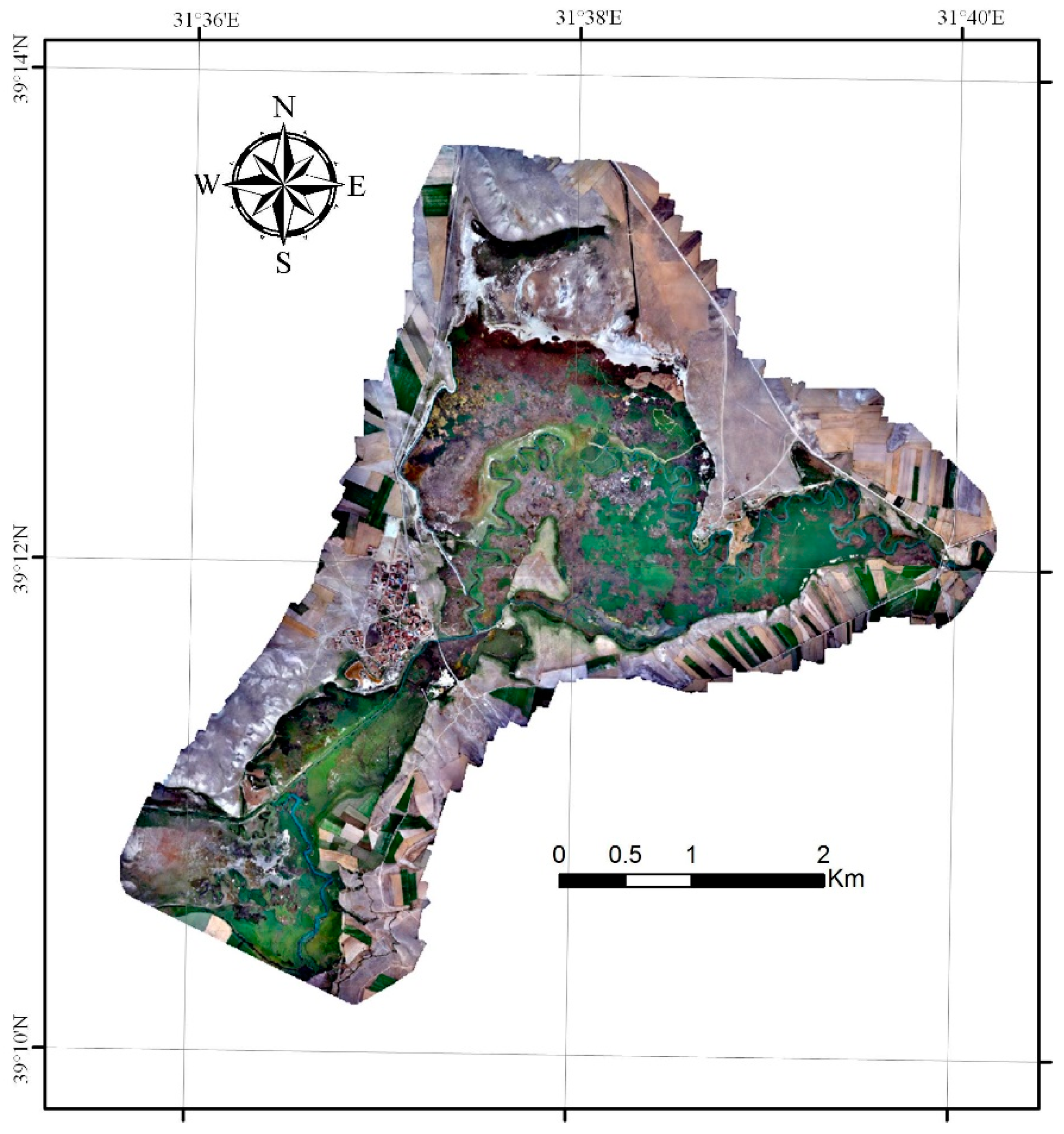
Sakarya River is the third longest river in Turkey and is 824 km length, while Balikdami is one of the wetlands formed along Sakarya riverbed. Located in the central Anatolian part in Turkey, Balikdami is a unique wetland containing rich flora and fauna and more than 256 bird species. This area is one of Turkey’s few wetlands, and it is one of the most important accommodation points for birds that migrate seasonally between northern and southern countries. The reed areas in Balikdami are used as a shelter and breeding area for many birds.
The central Anatolian region has natural vegetation cover that starts forming after a harsh winter. The vegetation cover starts drying in the summer season due to lack of rainfalls. It should be noted that in the study area, the leaf-on season starts in April and ends before November, while the leaf-off season is between November and March.
According to the yearly hydro-meteorological reports, the rainfalls in the Anatolian region in the 2017 winter season, has been slightly below the average amount, while the highest average temperature has been reported in the summer period, in July, with 26 °C.
The study area has been visited for inspection in April 2017. However, since the bigger part of the wetland was inaccessible, it was decided to collect high-resolution optical data from an Unmanned Aerial Vehicle (UAV), and afterward to determine the classes with a wetland expert.
2.2. UAV Data
The structure of Balikdami wetland is complex and contains several different classes of wetlands. In order to be able to separate and investigate the differences and relations between the classes, in a leaf-on season, data from UAV with a resolution of 8 cm were collected over the study area, Balikdami. UAV platforms are nowadays a valuable source of data for surveillance, inspection, mapping, and 3D modeling issues. New applications in the short- and close-range domain are introduced, being the UAVs low-cost alternatives to the classical manned aerial photogrammetry [
27]. Today the UAVs images and 3D data are used in many different fields such as forestry and agriculture [
28], archeology and cultural heritage, environmental surveying, traffic monitoring [
29], 3D reconstruction etc.
In this study, a UAV was used for collecting data over the Balikdami wetland area on August 10, 2017. The steps followed for obtaining the UAV data were: (i) Flight Planning; (ii) Taking real images; (iii) Data processing; and (iv) Results. The UAV and the integrated camera, as well as their characteristics, are given in
Table 1.
The data were processed in the Pix4D software. The details for every flight data are given in
Table 2 and the orthophoto mosaic of all flight is given in
Figure 1.
Using the high-resolution imagery obtained with the UAV, in consultation with a wetland expert, we were able to distinguish six different classes within the study area. The classes and their characteristics are given below in
Table 3.
In order to collect detailed information about every class separately, according to the area of the classes, a number of random points were created and the values from every month from both Landsat-8 and Sentinel-1 satellite images were obtained. A total of twenty-three satellite images were used in this paper (
Table 4).
The Sentinel-1 images were downloaded for every month of the year, while the images from Landsat-8 were downloaded only in the cloud-free condition. Some of the dates of both satellites are close to each other with only a few days’ difference. Images from both satellites represent one annual cycle. After the download of the images, NDVI was calculated and LST maps were obtained for the Landsat-8 images, while Sentinel-1 images were pre-processed.
2.3. LST Estimation
The LST has been retrieved using a tool developed in ERDAS Imagine. First, the top of atmospheric (TOA) spectral radiance (
Lλ) has been calculated using Equation (1).
where
represents the band-specific multiplicative rescaling factor
is the Band 10 image
is the band-specific additive rescaling factor, and
is the correction for
Band 10 [
30]. After the digital numbers (DNs) have been converted to reflection, the TIRS band data has been converted from spectral radiance to brightness temperature (BT) using the thermal constants provided in the metadata file Equation (2).
K1 and
K2 are taken from the Landsat 8 metadata file.
The calculation of
NDVI is needed for further calculation of the proportion of vegetation. The
NDVI equation for Landsat 8 bands is as given in Equation (3), where
Band 4 is the Red and
Band 5 is the near infra-red band.
The Proportion of Vegetation represents the fractional vegetation cover and it is calculated based on the
NDVI values (Equation (4)). Thus, NDVI values for vegetation and soil
are suggested to apply in global conditions [
31].
The emissivity can be calculated following Equation (5).
where
and
are the vegetation and soil emissivities, respectively, and
C represents the surface roughness (
C = 0 for homogenous and flat surfaces) taken as a constant value of 0.005 [
32]. The condition can be represented with the following formula and the emissivity constant values are; 0.991 for water, 0.962 for built-up areas, 0.966 for soil, and 0.973 for vegetated areas [
24].
Water class has been assigned, for NDVI values lower than 0, and the emissivity value of 0.991 should be assigned. NDVI values between 0 and 0.2, are considered to be soil, with an emissivity value of 0.996. NDVI values between 0.2 and 0.4 are considered to be mixtures of soil and vegetation cover, and in the case, when the NDVI value is greater than 0.4, it is considered to be covered with vegetation, and the value of 0.973 need to be assigned.
The LST or the emissivity-corrected land surface temperature
Ts is computed with Equation (7) [
33]:
where
Ts is the LST in Celsius,
λ is the wavelength of emitted radiance (for which the peak response and the average of the limiting wavelength (
λ = 10.895) [
34] will be used), and
is a constant calculated with Equation (8).
where
σ is the Boltzmann constant (1.38 × 10
−23 J/K), h is Planck’s constant (6.626 × 10
−34 J s), and c is the velocity of light (2.998 × 10⁸ m/s).
2.4. Sentinel-1 Pre-Processing
Images acquired by spacecraft sensors usually can be distorted in brightness and geometry as a result of a number of environmental circumstances and system factors [
35]. Before using the products in any analyses, the radiometric and geometric distortions should be removed, or minimized. In this study, the preprocessing of the Sentinel-1 SAR data with the Sentinel-1 Toolbox intergraded in SNAP contains few steps: (i). Data preparation; (ii). Radiometric Calibration; (iii). Multilooking; (iv). Spackle Reduction; (v). Terrain Correction; (vi). DN to dB Conversion.
The data preparation consists of selecting the study area, selecting the data type needed for the study, selecting the date, and downloading the SAR product. In this study, twelve Ground Range Detected (GRD) Interferometric Wide (IW) swath Sentinel-1 images taken over the Balikdami wetland in Turkey, were downloaded from the Copernicus Open Access Hub.
After the download, radiometric and terrain calibration, as well as speckle reduction on the images has been performed. Radiometric calibration corrects the SAR image so that the pixel values represent the radar backscatter of the reflected surface. Compared to the optical image data, the biggest difference in the appearance of radar imagery is its poor radiometric quality [
35], thus it is difficult to make a visual interpretation of a SAR image. Speckle can be caused by random constructive and destructive interference resulting in salt and pepper noise over the SAR image [
36]. As speckle is one of the biggest noise in SAR data, it should be reduced before performing any analyses. The products have been filtered with Lee Sigma filer 5 × 5 window size. Terrain correction geocodes the image by correcting SAR geometric distortions with the help of a digital elevation model (DEM) and it produces a map projected product. With Geocoding the image is being converted from Slant Range or Ground Range Geometry into a Map Coordinate System. Terrain correction corrects SAR geometry effects such as foreshortening, layover, and shadows. For the terrain correction, a Range Doppler Terrain Correction with a digital elevation model of 30 m has been used. All the pre-processing steps have been performed in the SNAP software by ESA using the Sentinel-1 toolbox. The digital number values have been converted into backscattering values in decibel (dB) scale following Equation (9).
where
is the digital number value of the image, and
is the backscattered value in dB.
2.5. Collecting Samples
The sample collection of every class (Swamp, Water, Bog, Land, Wetland Mixture, Sediment Bogs) has been performed using random points on every class using the UAV image. Thus, 88 random points were added to the swamp class, 14 to the water class, 158 to the bog class, 73 to the land class, 187 to the wetland mixture class, and 35 to the sediment bog class, making a total of 555 points. After the points were added, LST and NDVI values were extracted for all eleven Landsat-8 images, and VH and VV values were extracted for all twelve Sentinel-1 images. The average values and the standard deviation values were calculated for every class. The relations between the LST, NDVI and, SAR values were made on an annual level based on monthly periods.
3. Analyses and Discussion
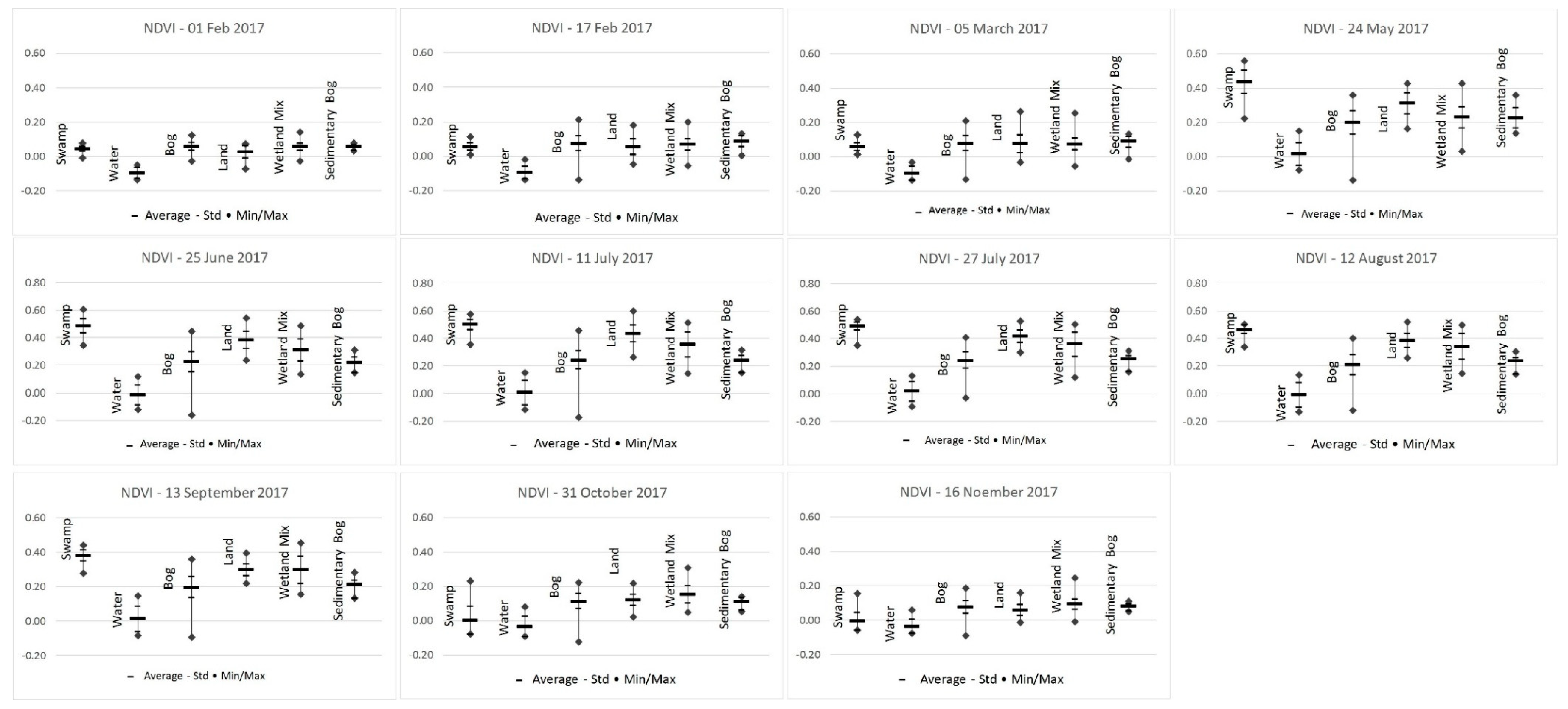
3.1. NDVI Results
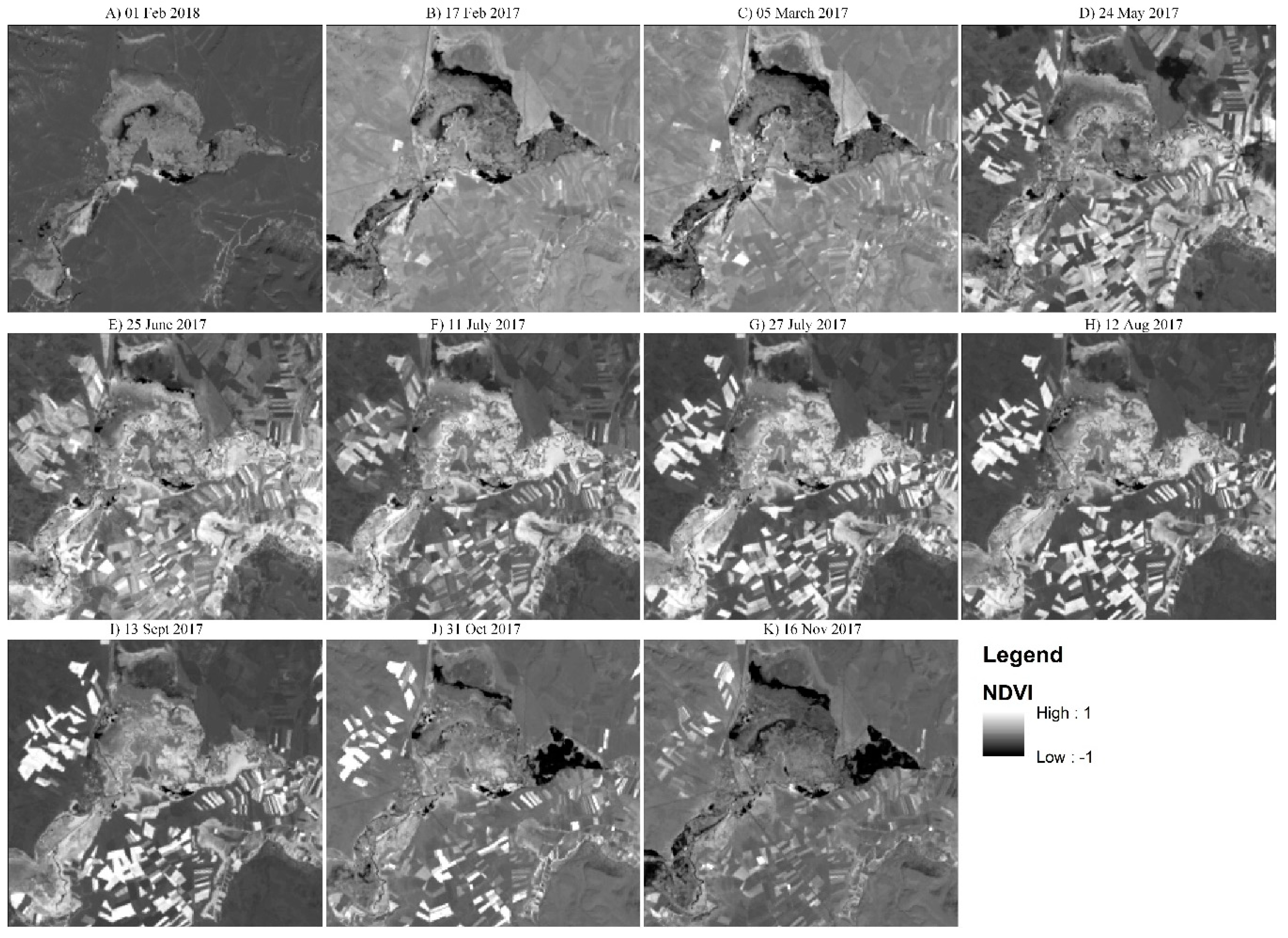
The pattern of NDVI time series has been closely analyzed in order to demonstrate its sensitivity in vegetation growth dynamics and its relation with LST and SAR data. As it is known, NDVI values vary from −1 to +1, where values smaller than 0 are classified as non-vegetated areas such as man-made objects, or water areas. Since in the study area no man-made objects were present, values lower than 0 were considered to be water areas. Values higher than 0 can be classified into three classes; values from 0–0.2 are considered to be bare lands, values from 0.2–0.4 are considered to be a mixture of land and small vegetation or unhealthy vegetation, while values higher from 0.4 are considered to be healthy vegetated areas. In
Figure 2,
Figure 3 and
Figure 4 are presented the NDVI time series results. Since the results of the same season months were similar, in
Figure 3, with respect to the date, the seasonal NDVI values of each class are compared. The full NDVI results are presented in
Figure A1.
As it can be seen from the NDVI results, every class taken into consideration in this study has different characteristics. As expected, the values of the water class are below or around zero. After March, when the leaf-on season begins, the NDVI value of the water class it is slightly above zero, indicating the presence of vegetation in the water. The NDVI value changes stay around zero depending on the water level until September, when the leaf-off season starts and the values drop below zero. The other five classes also tend to have low NDVI values at the beginning of the year, start to rise after March and stay stable until September, when the leaf-off season starts and the NDVI values drop. Swamps have the highest NDVI values generally varying from 0.4 to 0.6 in the leaf-on season. In the leaf-off season, NDVI value is close to zero and varying from slightly below zero to 0.2. The NDVI value of the Bog class can vary from −0.2 to 0.4 which makes is the most unstable wetland class in this study. The reason for this is the complex structure of Bogs, which contain soaked dry vegetation, wetlands, and shallow open water area. The NDVI values of the land class are much similar to the Swamp class, reaching the maximum NDVI value in July of 0.43. Similar to Bogs, the Wetland Mixture class defined in this study has a very complex structure. However, Wetland Mixture has higher NDVI values in the leaf-on season. Since there is the presence of small open water bodies, the NDVI values vary from slightly below zero to 0.3. The last class, Sediment Bog, is similar to the Bog class with the main difference of the land structure. While the land structure of Bog is formed of land, in the Sediment Bog the land is formed out of white sediment deposits formed over the years.
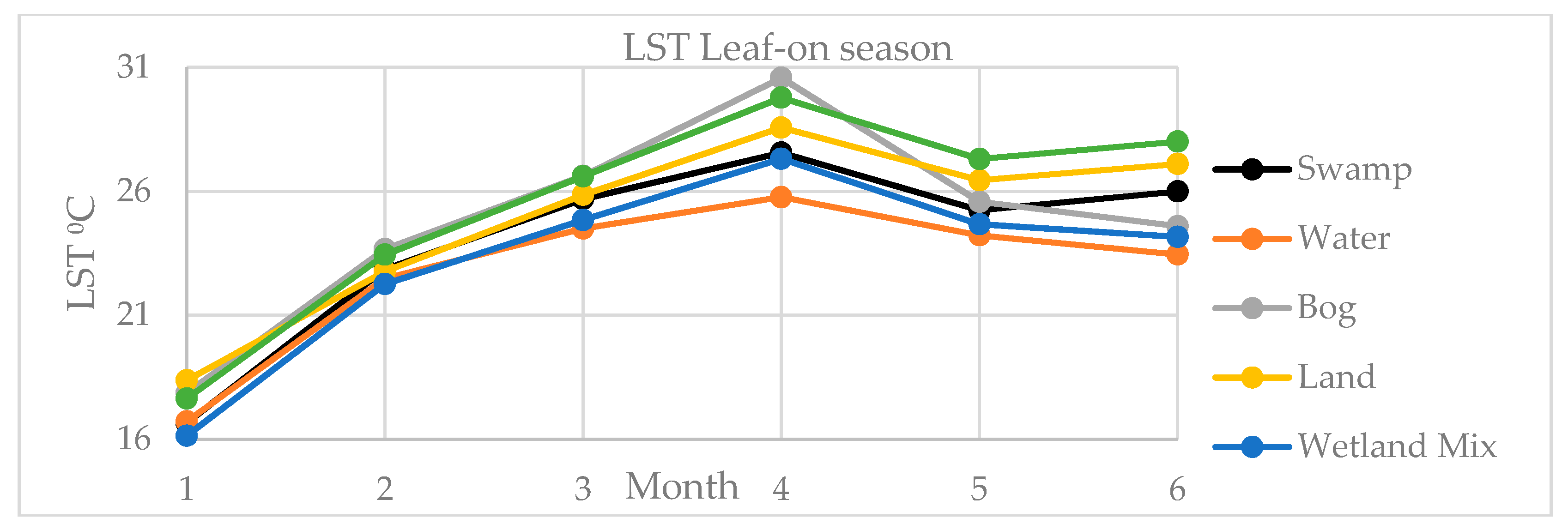
3.2. LST Results
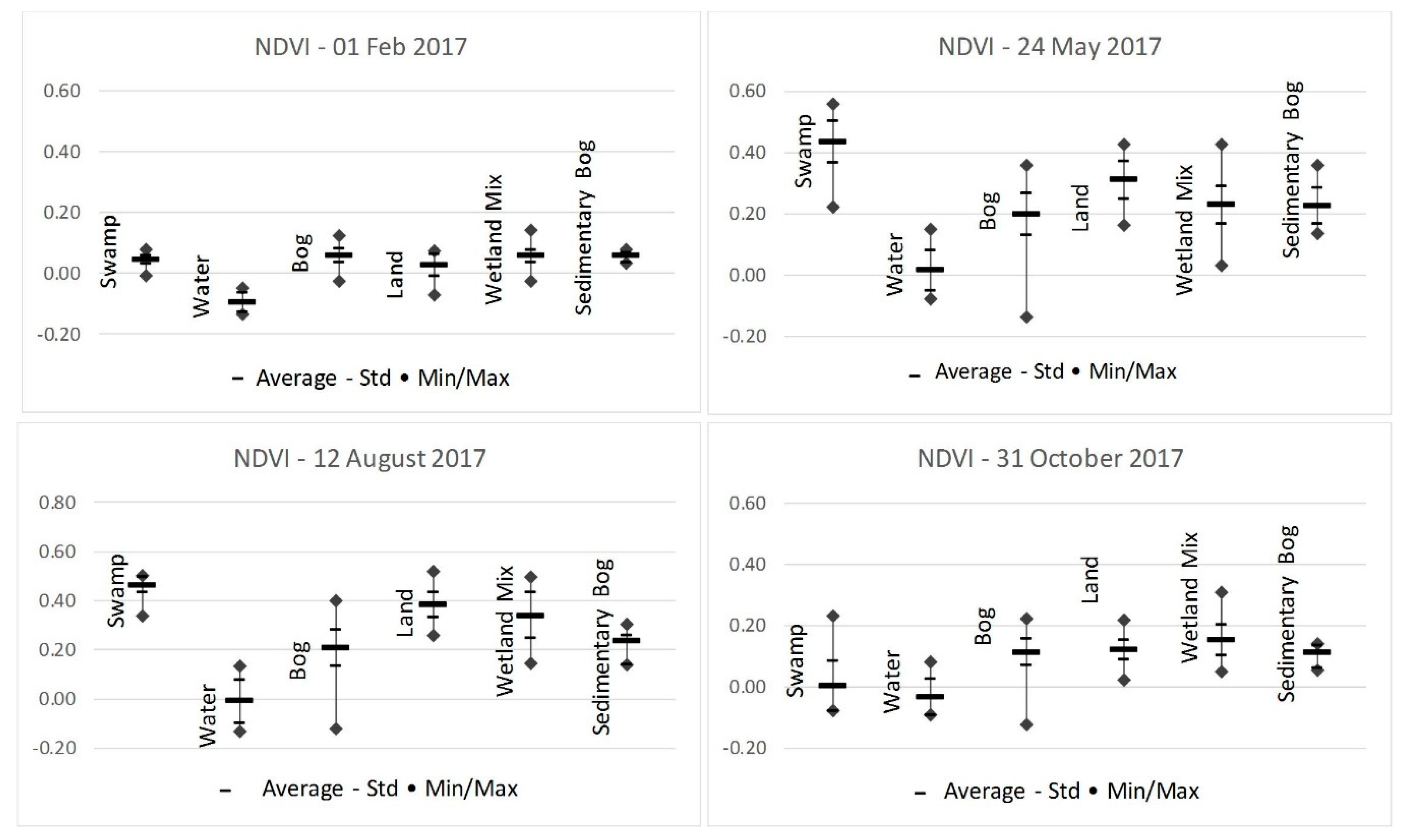
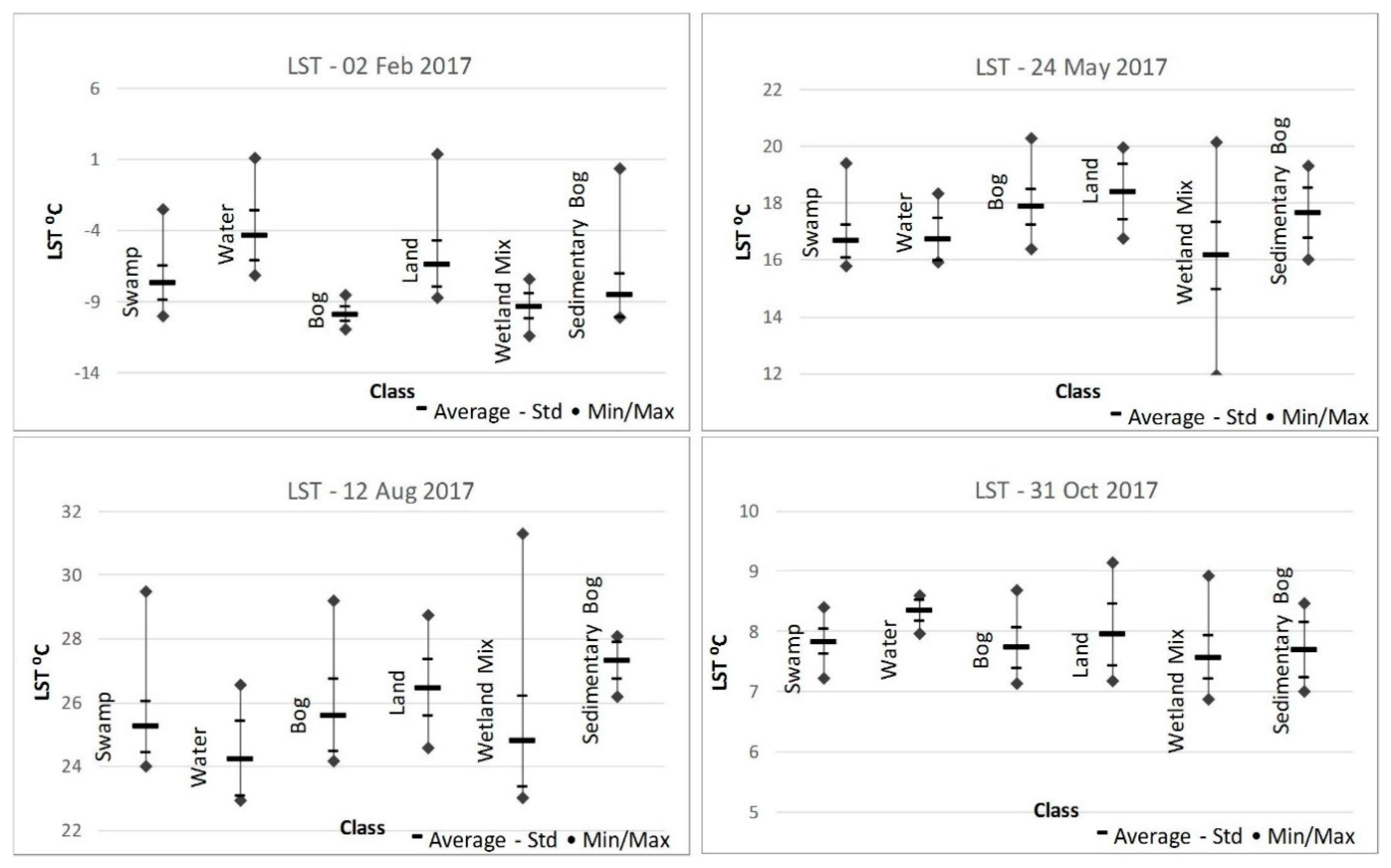
The results of the LST analyses can be seen in
Figure 5 and
Figure 6. The wetland area has temperatures below zero in the winter period and has its maximum temperature at the end of July for all classes. Compared with the average air temperatures of the central Anatolian region, the correlation is more than 0.9, which indicates that the LST of the wetland is substantially affected by the air temperature [
21]. The Water class has the highest temperature in the leaf-off season, and lowest in the leaf-on season. The full LST results are presented in
Figure A2.
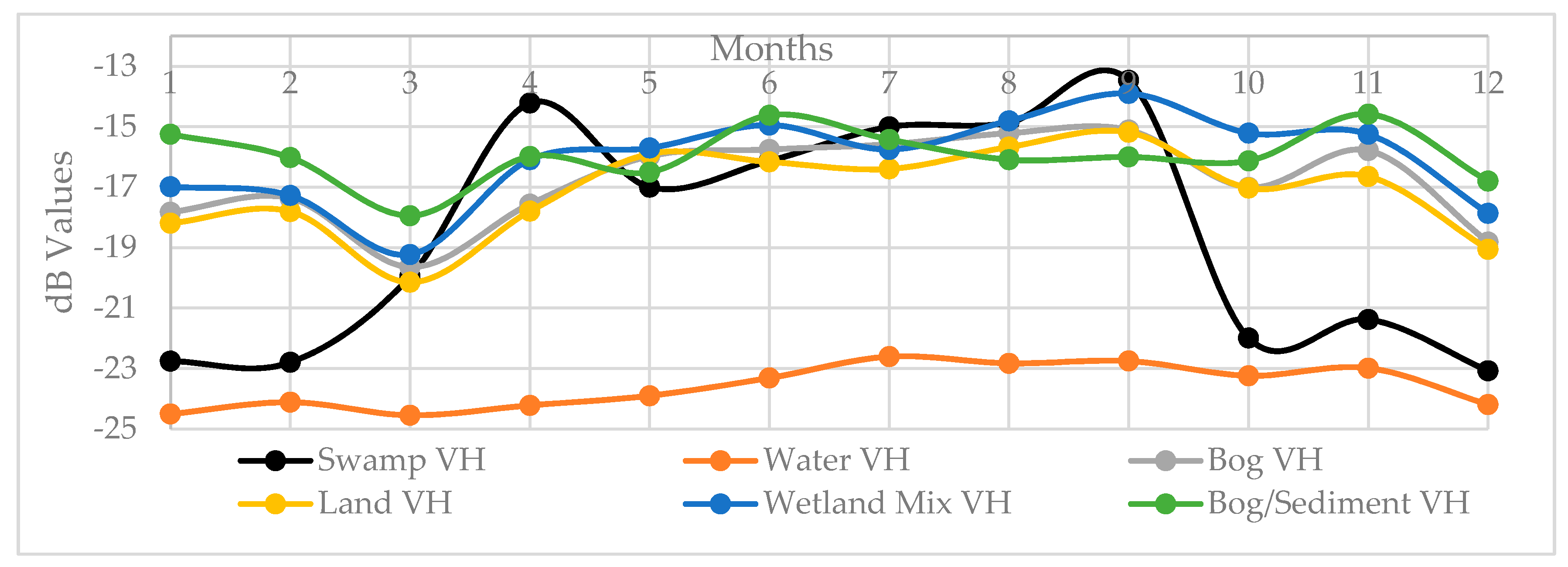
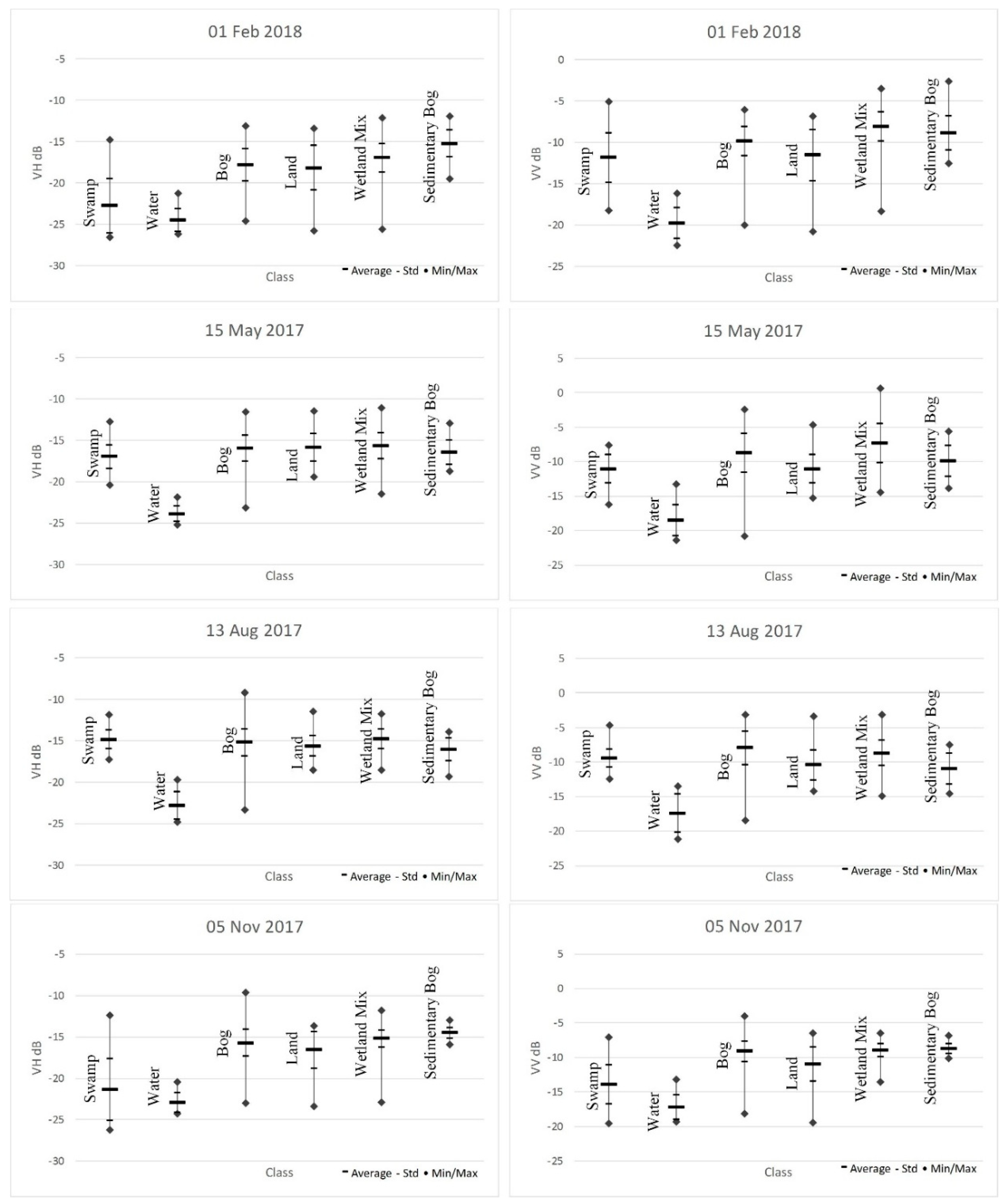
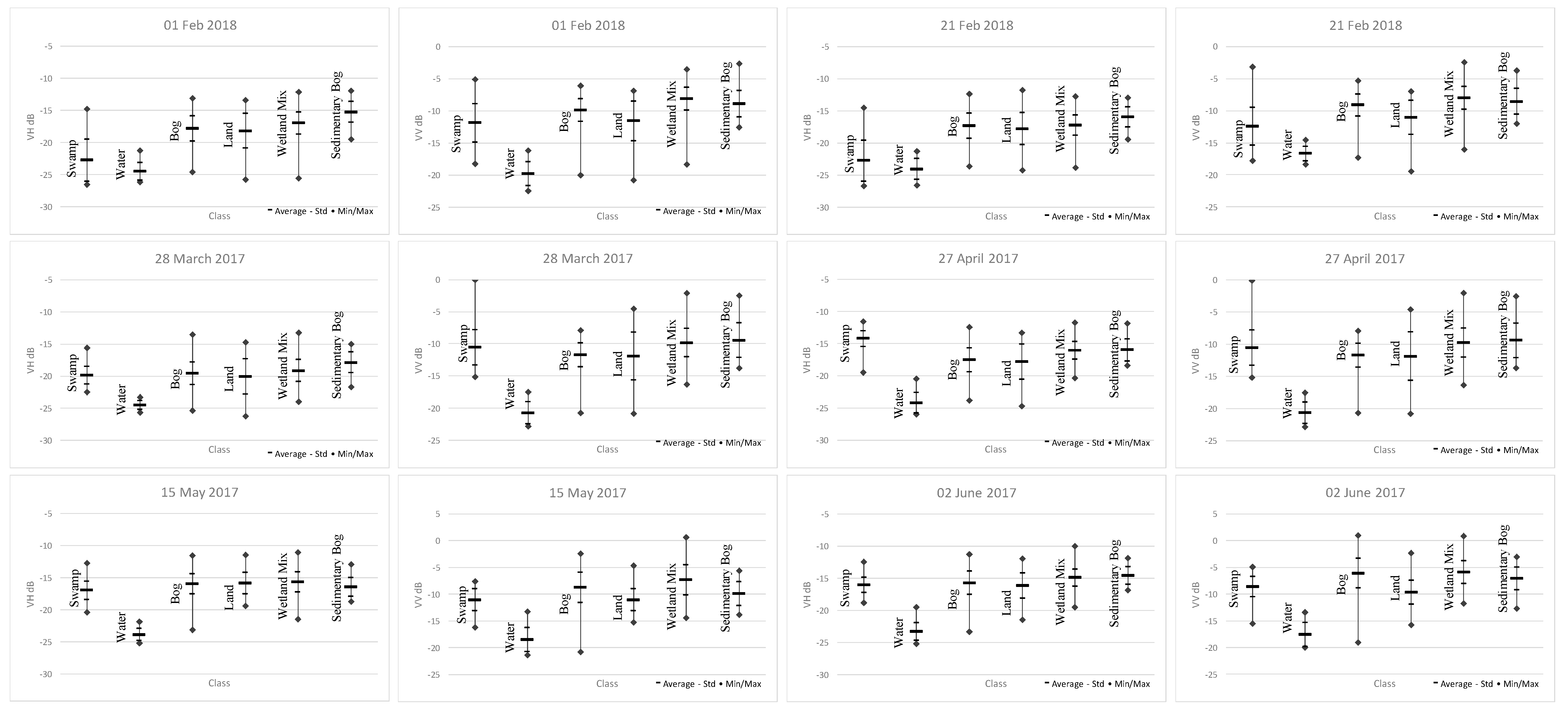
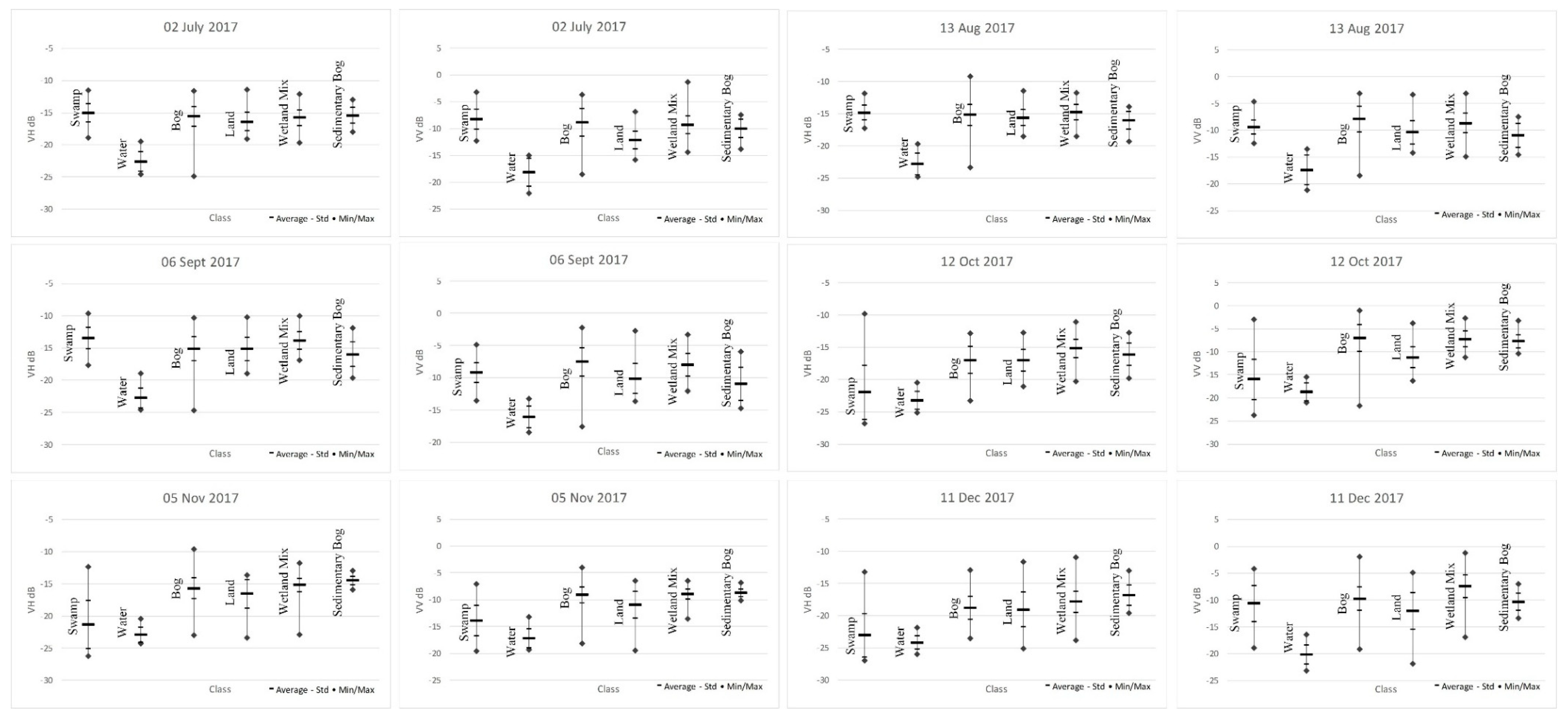
3.3. SAR Results
The results from the SAR data related to the monthly changes are presented in
Figure 7,
Figure 8 and
Figure 9. While the backscatter values of the water class, as expected, do not change much over the months, the other classes’ values vary depending on the vegetation growth. Thus, the values of the swamp class starts to rise up in March at the beginning of the leaf-on season and then drastically falls in October at the beginning of the leaf-off season. In the leaf-off season, the swamps are generally open water bodies, which explain the similar backscatter values with the water class. The other class values are similar to each other. However, the land class has the lowest backscatter values through the year except for August and September, when the bog/sediment class has the lowest values. The detailed comparison between the classes can be seen in
Figure A1,
Figure A2,
Figure A3 and
Figure A4.
3.4. LST, NDVI, and SAR Correlation
Several studies have investigated the correlation between the optical data and the SAR data for different land covers [
37,
38,
39]. In this study, the monthly correlation between the optical, thermal, and radar data within a wetland area was investigated. Thus, the average value of the eleven dates from Landsat-8, and the twelve dates from Sentinel-1 representing one year investigated in this study were taken into consideration for every class previously determined with the UAV data. The correlation results are presented in
Table 5. The full VH and VV results are presented in
Figure A3 and
Figure A4 respectively.
For the statistical comparison between the multi-sensor data were completed using correlation, which ranges between −1 (indirect relationship) and 1 (perfect relationship), and the correlations were supported using statistical significance variable which if it is less than 0.05 it means the results are significant—or that they did not just occur by chance.
It should be noted that the Landsat-8 and Sentinel-1 images were not taken at the same dates, but the used images present a one-year period presented with eleven images.
3.5. Discussion
In general terms, the complex structure of the wetlands, makes them a challenging land cover class for classification. As SAR sensors can often penetrate through herbaceous vegetation (C-band), the stronger backscatter signal is expected from wetter surfaces then the one from a drier surface [
37], thus the wetter surfaces are easier to identify through remote sensing techniques [
3], which makes the detection of open water bodies without vegetation relatively simple as weak or no signal returns to the antenna. When the water level is high or the wetlands are dominated by lower vegetation, the radar signal is often reduced [
40], while when the water level is low related to the vegetation, double-bounce scattering occurs [
41].
In this study, the backscatter VH values from the open water class range from −25 dB in the leaf-off season, and −23 dB in the pick of the leaf-on season, indicating low vegetation presence. Similar results are obtained from the VV polarization, with backscatter values ranging from −16 to −21 dB. The backscattering values of the other classes depend on both vegetation and water level. Thus, in the leaf-off season when the water level is high, the vegetation presence is low. The swamp class in the leaf-off season has low backscatter values, indicating low or no vegetation at all. Because of the medium resolution of both optical and radar sensors used in this study, the other classes include more heterogeneous land covers, which open a wide range of backscatter values and thus a mixture of the classes can occur.
While the NDVI and LST values only present the vegetation presence and the temperature in one pixel, relating them with data retrieved from a sensor with different characteristics as radar can be of great importance. As seen in
Table 5, the highest relation between the investigated characteristics has been noted in the NDVI-LST relation, which was expected as the LST calculation is directly connected to the NDVI values and several studies have found a strong correlation between them [
42]. The statistical results in this study also showed a strong statistically significant correlation between NDVI and LST. A strong correlation was also noted between the VH and the NDVI and LST data while there was no strong correlation between the VV polarization and the other investigated parameters, which is consistent with the report by Kwoun and Lu [
37], who used data from the European Remote-Sensing Satellites (ERS-1, VV polarization, C-band). There is no strong correlation between the investigated parameters in the Sediment Bog class because of its heterogenic structure where different land cover types can be found. This is also the case in the correlation between the VV and VH data in the Land, Wetland Mixture, and Sediment Bog class, where the correlations are not supported by the significance values. The results of Kasischke et al. [
17], who used a multi-year model to analyze the effects of seasonal hydrologic patterns in wetlands, indicated relatively little impact on the variation in biomass over the variation in backscatter values. Similar to this study, Zhang et al. [
15] used multi-temporal and multi-sensor data in order to identify the backscattering characteristics of wetland vegetation. Backscatter values of the reed marshes drastically increase at the beginning of the leaf-on season, from −10.8 dB to −2.1 dB at the VV polarization, which is similar to the findings of this study, where the values of the marsh class increase from −10.6 dB to −0.7 dB at the beginning of the leaf-on season at the VV polarization. In both of the studies, the reverse situation has been observed in the leaf-off season. Li et al. [
19] reported that Radarsat data can provide more accurate data than Landsat Thematic Mapper data for wetland biomass estimation. However, the best results can be obtained with a combination of the data. In the analyses of the backscatter signature in [
43], the maximum values occur when soil moisture is high and vegetation is fully developed with values of approximately −5 dB in the HH polarization, while the minimum occurs in the leaf-off season with values of approximately −20 dB. The results of the VH polarization in our study showed similar results, where the minimum value is −20.15 dB and the maximum −14.22 dB. Regarding the LST data, similar to the findings in Eisavi et al. [
21], this study also indicates that the land surface temperature of wetlands is substantially affected by the air temperature. In our study, we have confirmed this statement by finding the correlation between the average monthly air temperatures and land surface temperature, which is 0.9.
Observing the results in
Figure 7 and
Figure 8, as well as the statistical results in
Figure 9, beside their different characteristics, the spectral signature of the Land, Wetland Mix, Bog, and Sedimentary Bog are similar, and very unstable except for the Sedimentary Bog class in the leaf-off season. This corresponds to the low spatial resolution of the used remote sensing images because the majority of the pixels represents a mixture of several land/wetland cover types [
44].
4. Conclusions
The objective of this research was to investigate the LST and NDVI values obtained from Landsat 8 satellite, and VV and VH backscatter values obtained from the Sentinel-1 satellite, over a wetland area on a monthly basis and then to investigate the correlation between these values. Several studies have investigated and discussed the relation between backscatter and NDVI values in different classes. However, the relation between backscatter values and LST values in wetland classes have not been the subject of a detailed investigation. The results of this study show the dynamics of the investigated parameters within a wetland area where six different classes have been determined.
Comparing the LST results with a monthly average air temperature of the investigated region, the correlation is more than 0.9, indicating that the LST of the wetland is substantially affected by the air temperature. Following the LST values, NDVI values gave similar results with a correlation of nearly 0.9 in all classes.
Although the correlation between Landsat 8 and Sentinel-1 investigated parameters are not as high as the LST and NDVI values, and the images are not from the same dates, there is a strong relation between LST and NDVI, and VH backscatter values on a monthly basis. Similar to the findings of other research, VH polarization performs better than VV polarization in all of the investigated classes. For a better understanding of the relation, the wetland vegetation stage should be closely monitored. Thus, in the leaf-off season, when the vegetation is dry, or there is no presence of vegetation, the backscatter values represent the surface.
Although Sentinel-2 has better temporal, spatial, and spectral resolution with three additional bands red edge vegetation bands, Landsat-8 has been chosen in this paper because of its ability to collect data in the thermal wavelength region. For future studies, the correlation between Sentinel-1 and Sentinel-2 data in a wetland area should be investigated. Also, in order to clarify the representation of the satellite data in wetland areas, for future research, field measurements close to the image acquisition time are needed.


