Line-Constrained Shape Feature for Building Change Detection in VHR Remote Sensing Imagery

Abstract
1. Introduction
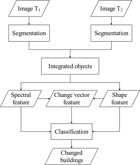
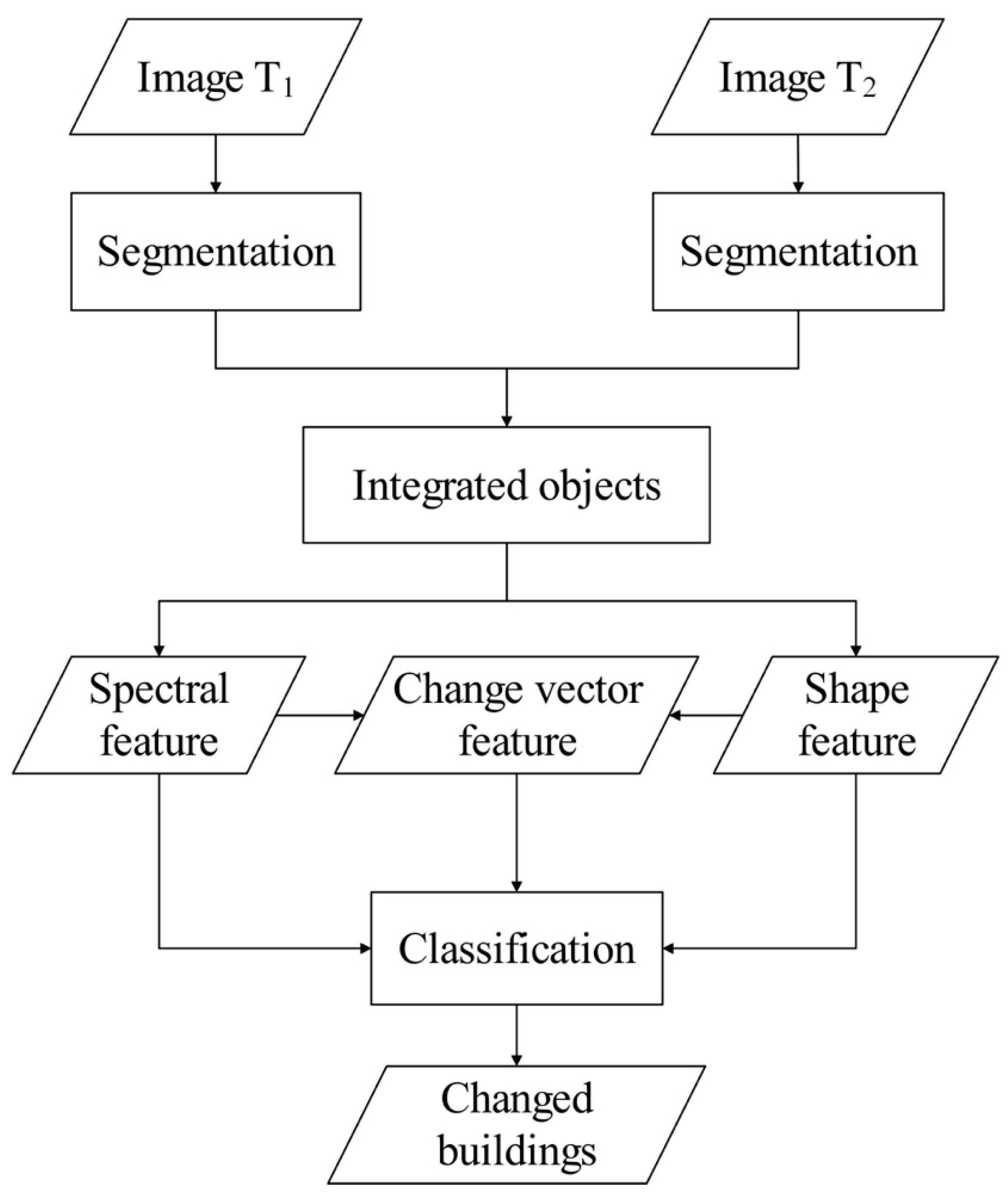
2. Methodology
2.1. Image Object Generation
2.2. Shape Feature Extraction
2.2.1. Building Likelihood Map
2.2.2. Building Candidate Area
2.2.3. Line-Constrained Shape Feature
2.3. Feature Vector Construction
2.4. Classification
3. Results and Discussion
3.1. Study Data
3.2. Evaluation Metrics
3.3. Parameter Setting
3.4. LCS Effect
3.5. Parameter Sensitivity Analysis
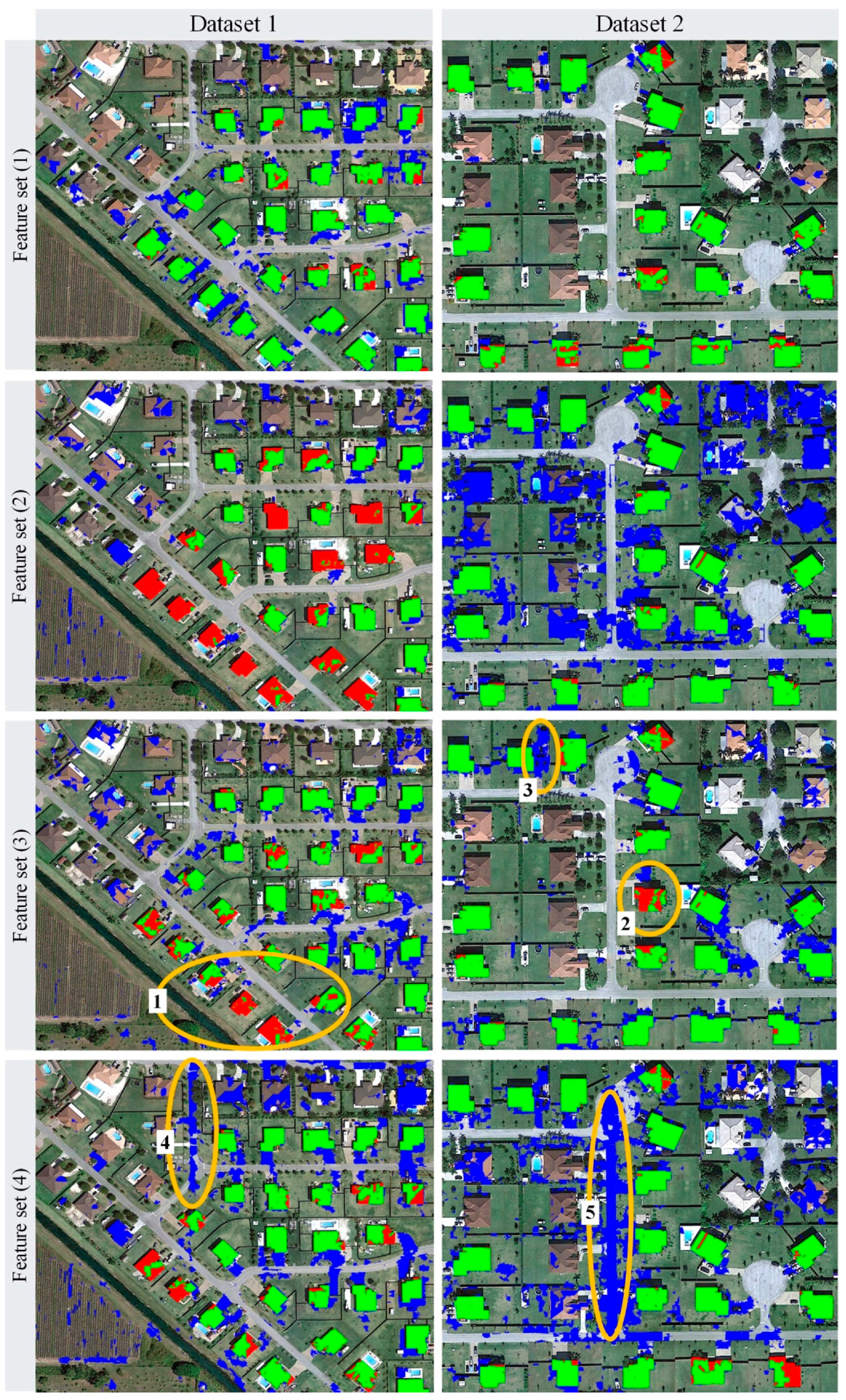
3.6. Comparison of Different Features
- (1)
- Spectrum + Shape (LCS) + Object (Spectra + Shape) CV
- (2)
- Spectrum + Object Spectra CV
- (3)
- Spectrum + Shape (PSI) + Object (Spectra + Shape) CV
- (4)
- Spectrum + Shape (MBI) + Object (Spectra + Shape) CV
4. Conclusions and Future Work
Author Contributions
Funding
Acknowledgments
Conflicts of Interest
Abbreviation
| BCA | building candidate area |
| BL | building likelihood |
| CV | change vector |
| LCS feature | line-constrained shape feature |
| LSD | line segment detector |
| MBI | morphological building index |
| POL | pixel on line segment |
| PSI | pixel shape index |
| SLIC | simple linear iterative clustering |
| FDR | false-detection rate |
| OA | overall accuracy |
| TA | thematic accuracy |
| UBCA | union building candidate area |
| VHR images | very-high-spatial resolution images |
References
- Wang, X.; Liu, S.; Du, P.; Liang, H.; Xia, J.; Li, Y. Object-Based Change Detection in Urban Areas from High Spatial Resolution Images Based on Multiple Features and Ensemble Learning. Remote Sens. 2018, 10, 276. [Google Scholar] [CrossRef]
- Tenedório, J.A.; Rebelo, C.; Estanqueiro, R.; Henriques, C.D.; Marques, L.; Gonçalves, J.A. New Developments in Geographical Information Technology for Urban and Spatial Planning. In Technologies for Urban and Spatial Planning: Virtual Cities and Territories; Pinto, N., Tenedório, J., Antunes, A., Cladera, J., Eds.; IGI Global: Hershey, PA, USA, 2014; pp. 196–227. [Google Scholar]
- Hussain, M.; Chen, D.; Cheng, A.; Wei, H.; Stanley, D. Change Detection from Remotely Sensed Images: From Pixel-Based to Object-Based Approaches. ISPRS J. Photogramm. Remote Sens. 2013, 80, 91–106. [Google Scholar] [CrossRef]
- Lu, D.; Mausel, P.; Brondízio, E.; Moran, E. Change Detection Techniques. Int. J. Remote Sens. 2004, 25, 2365–2401. [Google Scholar] [CrossRef]
- Singh, A. Digital change detection techniques using remotely-sensed data. Int. J. Remote Sens. 1989, 10, 989–1003. [Google Scholar] [CrossRef]
- Lunetta, R.S.; Johnson, D.M.; Lyon, J.G.; Crotwell, J. Impacts of imagery temporal frequency on land-cover change detection monitoring. Remote Sens. Environ. 2004, 89, 444–454. [Google Scholar] [CrossRef]
- Gang, C.; Geoffrey, J.H.; Luis, M.T.C.; Michael, A.W. Object-based change detection. Int. J. Remote Sens. 2012, 33, 4434–4457. [Google Scholar] [CrossRef]
- Bruzzone, L.; Bovolo, F. A novel framework for the design of change-detection systems for very-high-resolution remote sensing images. Proc. IEEE 2013, 101, 609–630. [Google Scholar] [CrossRef]
- Tewkesbury, A.P.; Comber, A.J.; Tate, N.J.; Lamb, A.; Fisher, P.F. A critical synthesis of remotely sensed optical image change detection techniques. Remote Sens. Environ. 2015, 160, 1–14. [Google Scholar] [CrossRef]
- Volpi, M.; Tuia, D.; Bovolo, F.; Kanevski, M.; Bruzzone, L. Supervised Change Detection in Vr Images Using Contextual Information and Support Vector Machines. Int. J. Appl. Earth Obs. Geoinf. 2013, 20, 77–85. [Google Scholar] [CrossRef]
- Coppin, P.; Jonckheere, I.; Nackaerts, K.; Muys, B.; Lambin, E. Digital Change Detection Methods in Ecosystem Monitoring: A Review. Int. J. Remote Sens. 2004, 25, 1565–1596. [Google Scholar] [CrossRef]
- İlsever, M.; Ünsalan, C. Two-Dimensional Change Detection Methods. SpringerBriefs Comput. Sci. 2012, 43, 469. [Google Scholar]
- Ma, L.; Li, M.; Blaschke, T.; Ma, X.; Tiede, D.; Cheng, L. Object-based change detection in urban areas: The effects of segmentation strategy, scale, and feature space on unsupervised methods. Remote Sens. 2016, 8, 761. [Google Scholar] [CrossRef]
- Plowright, A.; Tortini, R.; Coops, N.C. Determining Optimal Video Length for the Estimation of Building Height through Radial Displacement Measurement from Space. ISPRS Int. J. Geo-Inf. 2018, 7, 380. [Google Scholar] [CrossRef]
- Benz, U.C.; Hofmann, P.; Willhauck, G.; Lingenfelder, I.; Heynen, M. Multi-Resolution, Object-Oriented Fuzzy Analysis of Remote Sensing Data for Gis-Ready Information. ISPRS J. Photogramm. Remote Sens. 2004, 58, 239–258. [Google Scholar] [CrossRef]
- Blaschke, T. A Framework for Change Detection Based on Image Objects. Manuf. Eng. 2005, 73, 30–31. [Google Scholar]
- Tang, Y.; Zhang, L.; Huang, X. Object-Oriented Change Detection Based on the Kolmogorov–Smirnov Test Using High-Resolution Multispectral Imagery. Int. J. Remote Sens. 2011, 32, 5719–5740. [Google Scholar] [CrossRef]
- Huo, C.; Zhou, Z.; Lu, H.; Pan, C.; Chen, K. Fast Object-Level Change Detection for Vhr Images. IEEE Geosci. Remote Sens. Lett. 2010, 7, 118–122. [Google Scholar] [CrossRef]
- Xiao, P.; Zhang, X.; Wang, D.; Yuan, M.; Feng, X.; Kelly, M. Change Detection of Built-up Land: A Framework of Combining Pixel-Based Detection and Object-Based Recognition. ISPRS J. Photogramm. Remote Sens. 2016, 119, 402–414. [Google Scholar] [CrossRef]
- Kiema, J.B.K. Texture Analysis and Data Fusion in the Extraction of Topographic Objects from Satellite Imagery. Int. J. Remote Sens. 2002, 23, 767–776. [Google Scholar] [CrossRef]
- Myint, S.W.; Lam, N.S.N.; Tyler, J.M. Wavelets for Urban Spatial Feature Discrimination. Photogramm. Eng. Remote Sens. 2004, 70, 803–812. [Google Scholar] [CrossRef]
- Dell’Acqua, F.; Gamba, P.; Ferrari, A.; Palmason, J.A. Exploiting Spectral and Spatial Information in Hyperspectral Urban Data with High Resolution. Geosci. Remote Sens. Lett. IEEE 2004, 1, 322–326. [Google Scholar] [CrossRef]
- Kovács, A.; Szirányi, T. Improved harris feature point set for orientation-sensitive urban-area detection in aerial images. IEEE Geosci. Remote Sens. Lett. 2013, 10, 796–800. [Google Scholar] [CrossRef]
- Tao, C.; Tan, Y.; Zou, Z.R.; Tian, J. Unsupervised Detection of Built-up Areas from Multiple High-Resolution Remote Sensing Images. IEEE Geosci. Remote Sens. Lett. 2013, 10, 1300–1304. [Google Scholar] [CrossRef]
- Zhang, C.; Hu, Y.; Cui, W.H. Semiautomatic right-angle building extraction from very high-resolution aerial images using graph cuts with star shape constraint and regularization. J. Appl. Remote Sens. 2018, 12, 1. [Google Scholar] [CrossRef]
- Shackelford, A.K.; Davis, C.H. A Combined Fuzzy Pixel-Based and Object-Based Approach for Classification of High-Resolution Multispectral Data over Urban Areas. IEEE Trans. Geosci. Remote Sens. 2003, 41, 2354–2363. [Google Scholar] [CrossRef]
- Zhang, L.; Huang, X.; Huang, B.; Li, P. A Pixel Shape Index Coupled with Spectral Information for Classification of High Spatial Resolution Remotely Sensed Imagery. IEEE Trans. Geosci. Remote Sens. 2006, 44, 2950–2961. [Google Scholar] [CrossRef]
- Huang, X.; Zhang, L. Morphological Building/Shadow Index for Building Extraction from High-Resolution Imagery over Urban Areas. IEEE J. Sel. Top. Appl. Earth Obs. Remote Sens. 2012, 5, 161–172. [Google Scholar] [CrossRef]
- Xu, Z.; Wang, R.; Zhang, H.; Li, N.; Zhang, L. Building extraction from high-resolution sar imagery based on deep neural networks. Remote Sens. Lett. 2017, 8, 888–896. [Google Scholar] [CrossRef]
- Yang, H.L.; Yuan, J.; Lunga, D.; Laverdiere, M.; Rose, A.; Bhaduri, B. Building extraction at scale using convolutional neural network: Mapping of the united states. IEEE J. Sel. Top. Appl. Earth Obs. Remote Sens. 2018, 99, 1–15. [Google Scholar] [CrossRef]
- Shu, Z.; Hu, X.; Sun, J. Center-point-guided proposal generation for detection of small and dense buildings in aerial imagery. IEEE Geosci. Remote Sens. Lett. 2018, 15, 1100–1104. [Google Scholar] [CrossRef]
- Peng, F.; Gong, J.; Wang, L.; Wu, H.; Liu, P. A New Stereo Pair Disparity Index (Spdi) for Detecting Built-up Areas from High-Resolution Stereo Imagery. Remote Sens. 2017, 9, 633. [Google Scholar] [CrossRef]
- Huang, X.; Zhang, L.; Zhu, T. Building Change Detection from Multitemporal High-Resolution Remotely Sensed Images Based on a Morphological Building Index. IEEE J. Sel. Top. Appl. Earth Obs. Remote Sens. 2013, 7, 105–115. [Google Scholar] [CrossRef]
- Xiao, P.; Yuan, M.; Zhang, X.; Feng, X.; Guo, Y. Cosegmentation for Object-Based Building Change Detection from High-Resolution Remotely Sensed Images. IEEE Trans. Geosci. Remote Sens. 2017, 55, 1587–1603. [Google Scholar] [CrossRef]
- Tang, Y.; Huang, X.; Zhang, L. Fault-Tolerant Building Change Detection from Urban High-Resolution Remote Sensing Imagery. IEEE Geosci. Remote Sens. Lett. 2013, 10, 1060–1064. [Google Scholar] [CrossRef]
- Zhang, Q.; Huang, X.; Zhang, G. Urban Area Extraction by Regional and Line Segment Feature Fusion and Urban Morphology Analysis. Remote Sens. 2017, 9, 663. [Google Scholar] [CrossRef]
- Chen, J.; Deng, M.; Mei, X.; Chen, T.; Shao, Q.; Hong, L. Optimal Segmentation of a High-Resolution Remote-Sensing Image Guided by Area and Boundary. Int. J. Remote Sens. 2014, 35, 6914–6939. [Google Scholar] [CrossRef]
- Achanta, R.; Shaji, A.; Smith, K.; Lussichi, A.; Fua, P.; Susstrunk, S. SLIC superpixels compared to state-of-the-art superpixel methods. IEEE Trans. Pattern Anal. Mach. Intell. 2012, 34, 2274–2282. [Google Scholar] [CrossRef] [PubMed]
- Gioi, R.G.V.; Jakubowicz, J.; Morel, J.M.; Randall, G. Lsd: A line segment detector. Image Process. Line 2012, 2, 35–55. [Google Scholar] [CrossRef]
- Otsu, N. A Threshold Selection Method from Gray-Level Histograms. IEEE Trans. Syst. Man Cybern. 1979, 9, 62–66. [Google Scholar] [CrossRef]
- Dreiseitl, S.; Ohnomachado, L. Logistic regression and artificial neural network classification models: A methodology review. J. Biomed. Inform. 2002, 35, 352–359. [Google Scholar] [CrossRef]
- Jensen, J.R. Introductory Digital Image Processing: A Remote Sensing Perspective; Prentice-Hall: Upper Saddle River, NJ, USA. 2004; p. 382. [Google Scholar]
- Freire, S.; Santos, T.; Navarro, A.; Soares, F.; Silva, J.D.; Afonso, N. Introducing mapping standards in the quality assessment of buildings extracted from very high resolution satellite imagery. ISPRS J. Photogramm. Remote Sens. 2014, 90, 1–9. [Google Scholar] [CrossRef]


| Number of Pixels | Real Changed | Real Unchanged | Total |
|---|---|---|---|
| Detected as changed | True positive (TP) | False positive (FP) | |
| Detected as unchanged | False negative (FN) | True negative (TN) | |
| Total | N |
| ω | Coverage Ratio in Image 2011 | Coverage Ratio in Image 2016 | Recall | FDR | OA | Kappa | TA |
|---|---|---|---|---|---|---|---|
| 10 | 92.51% | 92.79% | 74.66% | 1.25% | 96.35% | 0.7832 | 0.6712 |
| 50 | 99.14% | 97.33% | 87.74% | 1.41% | 97.51% | 0.8618 | 0.7787 |
| 90 | 99.02% | 88.11% | 81.22% | 1.44% | 96.82% | 0.8188 | 0.7187 |
| Dataset 1 | Dataset 2 | |||||||||
|---|---|---|---|---|---|---|---|---|---|---|
| Feature Sets | Recall | FDR | OA | Kappa | TA | Recall | FDR | OA | Kappa | TA |
| (1) | 91.57% | 5.79% | 93.97% | 0.7061 | 0.5858 | 87.74% | 1.41% | 97.51% | 0.8618 | 0.7787 |
| (2) | 48.03% | 4.12% | 91.42% | 0.4637 | 0.3427 | 95.67% | 19.06% | 82.14% | 0.4393 | 0.3521 |
| (3) | 74.68% | 6.88% | 91.4% | 0.5713 | 0.4473 | 91.03% | 6.53% | 93.22% | 0.6916 | 0.5731 |
| (4) | 83.8% | 10.62% | 88.86% | 0.5261 | 0.4121 | 91.57% | 17.04% | 83.82% | 0.4531 | 0.3612 |
© 2018 by the authors. Licensee MDPI, Basel, Switzerland. This article is an open access article distributed under the terms and conditions of the Creative Commons Attribution (CC BY) license (http://creativecommons.org/licenses/by/4.0/).
Share and Cite
Liu, H.; Yang, M.; Chen, J.; Hou, J.; Deng, M. Line-Constrained Shape Feature for Building Change Detection in VHR Remote Sensing Imagery. ISPRS Int. J. Geo-Inf. 2018, 7, 410. https://doi.org/10.3390/ijgi7100410
Liu H, Yang M, Chen J, Hou J, Deng M. Line-Constrained Shape Feature for Building Change Detection in VHR Remote Sensing Imagery. ISPRS International Journal of Geo-Information. 2018; 7(10):410. https://doi.org/10.3390/ijgi7100410
Chicago/Turabian StyleLiu, Haifei, Minhua Yang, Jie Chen, Jialiang Hou, and Min Deng. 2018. "Line-Constrained Shape Feature for Building Change Detection in VHR Remote Sensing Imagery" ISPRS International Journal of Geo-Information 7, no. 10: 410. https://doi.org/10.3390/ijgi7100410
APA StyleLiu, H., Yang, M., Chen, J., Hou, J., & Deng, M. (2018). Line-Constrained Shape Feature for Building Change Detection in VHR Remote Sensing Imagery. ISPRS International Journal of Geo-Information, 7(10), 410. https://doi.org/10.3390/ijgi7100410