Automated Identification of Discrepancies between Nautical Charts and Survey Soundings

Abstract

Timely and accurate identification of change detection for areas depicted on nautical charts constitutes a key task for marine cartographic agencies in supporting maritime safety. Such a task is usually achieved through manual or semi-automated processes, based on best practices developed over the years requiring a substantial level of human commitment (i.e., to visually compare the chart with the new collected data or to analyze the result of intermediate products). This work describes an algorithm that aims to largely automate the change identification process as well as to reduce its subjective component. Through the selective derivation of a set of depth points from a nautical chart, a triangulated irregular network is created to apply a preliminary tilted-triangle test to all the input survey soundings. Given the complexity of a modern nautical chart, a set of feature-specific, point-in-polygon tests are then performed. As output, the algorithm provides danger-to-navigation candidates, chart discrepancies, and a subset of features that requires human evaluation. The algorithm has been successfully tested with real-world electronic navigational charts and survey datasets. In parallel to the research development, a prototype application implementing the algorithm was created and made publicly available.

1. Introduction

The content of a nautical chart is derived from data sources that may greatly vary in both quality and density [1,2]. It is also common to have, in the same nautical chart, parts based on modern high-resolution hydrographic surveys coexisting with areas that have not been resurveyed since eighteenth-century lead-line surveys [3]. At the same time, the recent evolution of shipping has both widened and increased the hydrographic needs, with new harbors and routes established in areas that had never been surveyed [4]. Furthermore, on the other side, reasons of economic effectiveness cause merchant vessels to venture into approaches with less under keel clearance than before [3]. In addition, various natural events (e.g., hurricanes, high sedimentation rates) and human activities (e.g., dredging) may modify the condition of the premises and suddenly make parts or, in extreme cases, the entirety of a chart obsolete [5,6]. Thus, not only the quality of a nautical chart depends on the surveys upon which it is derived but surveying for avoiding chart obsolescence represents a never-ending task.

After a survey, the newly collected datasets are evaluated for evidence of substantial changes against the latest relevant nautical charts. This operation must take into account the numerous transformations that a survey sounding has undergone from the moment that a sonar ping is emitted to its final representation on the chart, in particular when integrated on a statistically-based bathymetric surface and as the consequence of several possible cartographic adjustments (rounding and truncation, generalization, etc.) [7,8,9,10]. In addition, although ontologically distinct, disentangling inaccuracy and uncertainty adds complexity to the already challenging scenario [11]. Concurrently, a general acceleration in the expected change rate of geospatial information during the past years pushes toward a much shorter updating cycle of nautical charts and, thus, a quick identification of discrepancies for a rapid dissemination of the required nautical information [2,3]. The identification of all the dangers to navigation (DtoNs) and navigationally significant features represents a challenge in complex surveys and significantly contributes to the total processing time of a newly collected dataset [7]. The timely and accurate detection of the above represents a key task for cartographic agencies to fulfill their paramount objective to support the safety of navigation in the relevant waters.

Such a task is complicated by the intrinsic complex nature of a nautical chart as the result of a varying combination of human-driven considerations at the compilation time. Those considerations typically change from offshore to inshore, or along an open shoreline toward an intricate estuary [1]. Overall, the main criterion driving the chart compilation is the usefulness to the mariner in relation to the scale of the chart and the surrounding details [1]. Following such a criterion, a less significant feature is generally excluded (or reduced in emphasis) when its insertion may obscure other more important charted elements. In areas where detailed bathy-morphological information is required, a nautical chart provides a careful selection of trend-meaningful charted soundings and depth contours. This selection allows the chart user to interpret the morphology of the seabed by interpolating the provided bathymetric information in accordance with the shoal-biased source survey datasets. The nature of the interpolation is delegated to the end user, and it can be assumed that this mental process varies from a plain linear interpolation to a heavily biased interpolation toward the conservative side. The degree of bias is a combination of—both objective and subjective—contingent user considerations and, as such, difficult to estimate. Together with the degree of interpolation bias, the likely existence of a few special cases related to the presence of feature types like marine farms, restricted areas, and other types of obstructions, complicates the identification of discrepancies between nautical charts and the survey soundings [12].

The evaluation of current chart adequacy (as well as the rectification of possible deficiencies and shortcomings) represents a worldwide pressing need that poses a challenge to many national hydrographic offices [13,14]. These offices must balance such a pressing need with the limited available resources and survey priorities. This translates to the fact that decades may past until a new hydrographic survey can be conducted in a given area. In such an optic, it is becoming more and more obvious that evaluating the adequacy of the chart portfolio requires not only using newly collected bathymetric sonar bathymetry (BSB) but any possible source of geospatial information like automatic-identification system (AIS) data or alternative surveying means such as synthetic aperture radar (SAR) shoreline extraction, satellite-derived bathymetry (SDB), and airborne-lidar bathymetry (ALB) [6,14,15,16,17,18,19,20]. However, given the physically-limited penetration in water of SAR, SDB, and ALB as well as the circular limitation in retrieving information from AIS data (i.e., vessels tend to avoid uncharted areas), BSB surveys—despite their high cost and logistic challenges—not only provide both highly accurate and dense measurements of the seafloor morphology, but also represent the only practical source of hydrographic information for large parts of the ocean [15].

The identification of nautical chart discrepancies in comparison to newly collected hydrographic survey datasets has received only limited attention in the scientific literature despite its importance for the safety of navigation and relevance in the evaluation of the adequacy of the current charts, as well as for coastal change analysis and coastal zone management [21,22,23,24,25]. In addition, many of the techniques developed for geospatial data analysis on land cannot be directly applied to the nautical cartography realm, mainly because of the peculiar safety of navigation requirement [12,26,27,28,29]. Currently, the task to identify chart discrepancies against new BSB data sets is usually performed by the various cartographic agencies through manual or semi-automated processes, based on best practices developed over the years. However, these processes require a substantial level of human commitment that includes the visual comparison of the chart against the new data, the analysis of intermediate support products or, more commonly, a combination of the two.

This work describes an algorithm that aims to automate a large extent of the change detection process and to reduce its subjective human component. Through the selective derivation of a set of depth points from a nautical chart, a triangulated irregular network (TIN) is created to apply a preliminary tilted-triangle test to all the input survey soundings. Given the complexity of a modern nautical chart, a set of additional sounding-in-specific-feature tests are then performed. As output, the algorithm provides DtoN candidates, chart discrepancies (the “deep” discrepancies may be optionally identified), and a subset of features that requires human evaluation (if any). The algorithm has been successfully tested with real-world Electronic Navigational Charts (ENCs) and survey datasets. In parallel to the development of this work, an application implementing the algorithm was created and made publicly available in the HydrOffice framework (https://www.hydroffice.org/catools).

2. Materials and Methods

2.1. Electronic Navigational Charts

An ENC provides all the information for safe navigation in the form of a database—standardized as to content, structure, and format—issued on the authority of government-authorized hydrographic offices [30]. As such, it does not only contain information for safe navigation present in the corresponding paper chart but can embed supplementary material present in other kinds of nautical publications (e.g., sailing directions). The ENC content may be directly derived from original survey material, but also from databased information, existing paper charts, or a combination of them [31].

The International Hydrographic Organization (IHO) has created a standard vector format, named S-57, for official ENCs (that is, produced by a government hydrographic office) that contain a set of data layers for a range of hydrographic applications. However, an IHO S-57 ENC is mainly used, in combination with positional information from navigation sensors and radar data, by an Electronic Chart Display and Information System (ECDIS) to provide a graphical representation of a marine area, including bathymetry and topography, and to assist the mariner in route planning and monitoring by providing natural features, man-made structures, coastlines, and any other information related to marine navigation [6,32]. To meet high standards of reliability and performance, an extensive body of rules defines an ECDIS with the result that, under SOLAS Chapter V regulations, an ECDIS loaded with official ENCs is currently the only alternative for the navigator to the adequate and up-to-date paper charts [33].

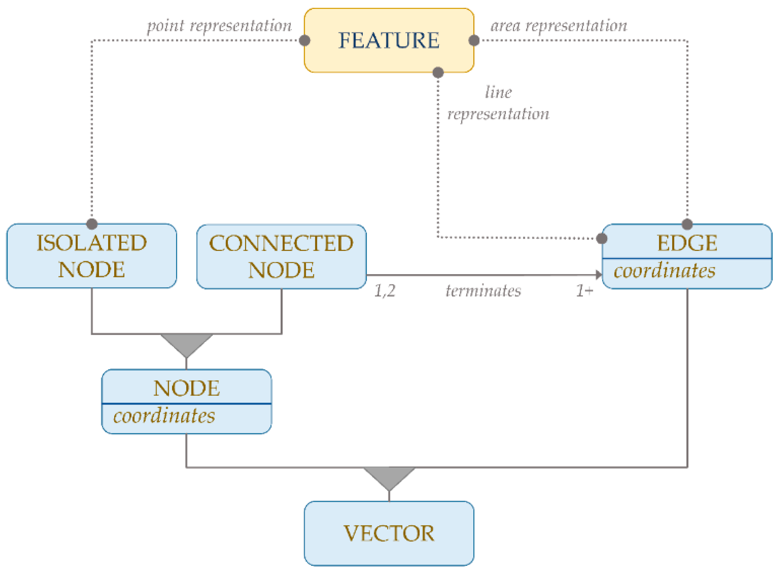
As defined by the IHO standard, the S-57 data content consists of a set of features that may have a spatial representation in the form of points, lines or polygons. Based on the ENC product specifications, those features must be encoded using the chain-node topology, as shown in Figure 1 [32,34]. For an S-57 ENC, the basic unit of geographic coverage is called “cell”, normally a spherical rectangle bordered by meridians and latitudes with actual data coverage of any shape [31]. Within the same navigational purpose (e.g., coastal, approach), see

Table 1. The Electronic Navigational Chart (ENC) navigational purposes with range of compilation scales (and the standard radar scale within each range) suggested by the International Hydrographic Organization(IHO) S-65 publication [31].

ENC Navigational Purpose	Suggested Scale Range	Selectable Radar Range	Rounded Standard Scale
Overview	<1:1,499,999	200 NM	1:3,000,000
		96 NM	1:1,500,000
General	1:350,000–1:1,499,999	48 NM	1:700,000
		24 NM	1:350,000
Coastal	1:90,000–1:349,999	12 NM	1:180,000
		6 NM	1:90,000
Approach	1:22,000–1:89,999	3 NM	1:45,000
		1.5 NM	1:22,000
Harbour	1:4,000–1:21,999	0.75 NM	1:12,000
		0.5 NM	1:8000
Berthing	>1:4000	0.25 NM	1:4000

, the cell data may not overlap with those of the adjacent cells. The navigational purpose also drives the compilation scale and, thus, the features contained in a cell.

2.2. Soundings from Bathymetric Sonar Surveys

In the hydrographic field, a sounding can be intended as a measured depth of water (i.e., a survey sounding) or as a bathymetric value represented on a nautical chart (i.e., a charted sounding) [30]. The algorithm described in this work digests both kinds of soundings, but with distinct uses. In fact, the survey soundings collected using bathymetric sonars—with multibeam sonars (MBES) currently playing a predominant role as acquisition devices—are analyzed as proxies for the bathy-morphology of the surveyed area [35], while the charted soundings represent one of the many feature types retrieved from the ENC to reconstruct the bathymetric model that the nautical cartographer wanted to communicate at the time of the ENC compilation (and, when present, after the application of all of the available ENC updates).

The algorithm described in this work was developed to handle the following types of survey soundings as the input:

• “Pure survey soundings”, intended as the point cloud measured by a bathymetric sonar after having been properly integrated with ancillary sensors, cleaned by spurious measurements, and reduced to the chart datum.
• “Gridded survey soundings”, represented by the nodes with valid depth values in a regularly-spaced grid created using the pure survey soundings.
• “Selected gridded survey soundings”, commonly generated during the cartographic processing using algorithms that select the grid nodes that are more meaningful to depict the trend of the underlining bathymetric model.

Assuming the correctness in the generation of the above three types of survey soundings (whose evaluation is outside of the scope of the present work), the algorithm provides similar output results, with the only relevant difference in the number of flagged features. The latter is justified by the different number of survey soundings in the input: The gridding and the selection processes commonly reduce the number of features input by one or more orders of magnitude.

2.3. Bathymetric Model Reconstruction using a Triangulated Irregular Network (TIN)

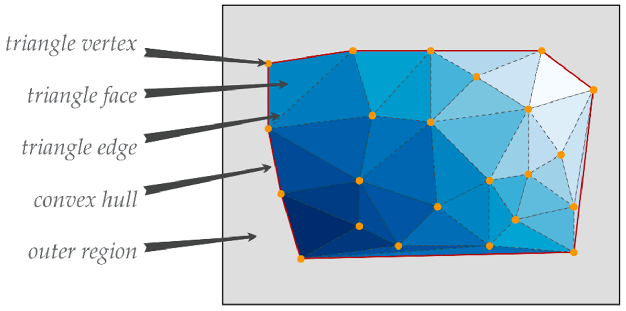
From a general point of view, a TIN consists of a network of irregular triangles generated by connecting the nodes of a dataset in a way that guarantees the absence of intersecting triangle edges and superposed triangle faces, but also ensuring that the union of all the triangles fills up the convex hull of the triangulation, see Figure 2 [36]. For the aims of this work, we generate a TIN from a set of three-dimensional nodes retrieved from the chart and then assume a linear variation of the bathymetric model among those nodes.

The generated TIN is based on the Delaunay conforming triangulation [37] selected for its well-known characteristic properties (e.g., being mathematically well defined, providing a unique output for a given dataset independently from the data sequence) [38]. In the literature, several algorithms implementing such a triangulation are available [39,40]. For the present work, we adopted the practical convex hull algorithm that combines the two-dimensional Quickhull algorithm with the general-dimension Beneath-Beyond algorithm, using the implementation provided by the open source QHull code library [41].

For the bathymetric model reconstruction, the algorithm retrieves nodes from the following ENC feature types (in parenthesis, the adopted S-57 acronym):

• Charted soundings (SOUNDG).
• Depth contour lines (DEPCNT) with a valid depth value attribute (VALDCO).
• Dredged area polygons (DRGARE) with a valid value for the minimum depth range attribute (DRVAL1).
• All the point features with a valid value of sounding attribute (VALSOU).
• Natural (COALNE) and artificial (SLCONS) shorelines.
• Depth area polygons (DEPARE) for the ENC cell boundaries only.

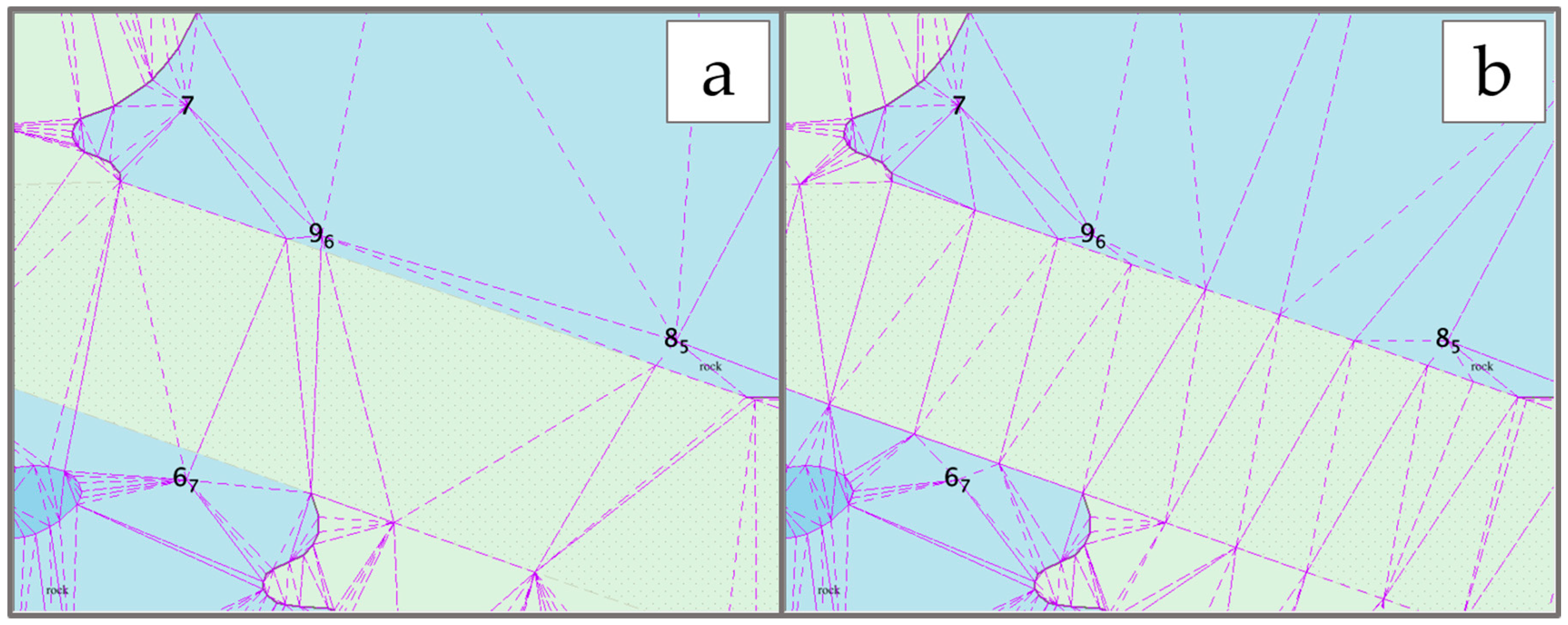
To avoid the creation of triangles crossing feature edges (and, thus, the corresponding misrepresentation in the reconstructed bathymetric model), additional nodes are inserted along the feature edges that are longer than the interpolation length ($IL$) of one centimeter ($k_{1cm}=0.01m$) at the ENC compilation scale ($CS$), see Figure 3:

$$IL=\frac{k_{1cm}}{CS}$$

(1)

For example, with a $CS$ value of 1:10,000, the $IL$ obtained by applying (1) is 100 m. Given that the position of the features in an ENC are provided as geographic coordinates referred to the World Geodetic System 1984 Datum (WGS84), the metrical $IL$ value is then converted to its corresponding geographic value using the local latitude [31,32].

The algorithm retrieves the $CS$ for (1) directly from the ENC, using the value stored in the “Compilation Scale of Data” (S-57 label: CSCL) subfield in the “Data Set Parameter” (S-57 field tag: DSPM) field structure [32]. By definition, such a value represents the compilation scale appropriate to the greater part of the data in the cell [32]. The derivation of the interpolation factor, $k$, from the ENC analysis (i.e., by looking at the distribution of the distance among the features) was attempted, but it did not provide satisfying results, mainly because of the intrinsic variable-resolution nature of a nautical chart. The 1-cm interpolation value was then established heuristically as a trade-off value between the requirement of avoiding the triangle-crossing-edge condition and the performance cost paid for a larger point cloud to triangulate. The effectiveness of $k_{1cm}$ has been empirically tested using real-world ENCs, but more conservative values for $k$—or its derivation from more advanced ENC analysis (e.g., locally estimating $k$ rather than attempting to define a single value for the full chart)—may be adopted.

In addition to the described point densification, the reconstruction of a bathymetric model from an ENC requires the association of a depth value to the nodes derived from the shoreline features, and that such a value is referenced to the chart vertical datum like all the other depth nodes. Given that chart producers may adopt different methods to identify the shoreline, the algorithm takes the depth value for the shoreline as an input parameter. However, if not provided, the algorithm defaults to use the shallowest depth value among all the valid depth values in the collected nodes.

The boundaries of the ENC bathymetry may be defined by the shoreline features and by the cell data limits. In this latter case, based on the enforced chain-node topology, the algorithm retrieves the nodes delimiting the point cloud by intersecting the depth area polygons along the cell boundaries with the depth contour lines. At the resulting nodes, the value of the minimum depth range attribute (S-57 acronym: DRVAL1) is assigned. In the rare cases where such a value is not populated in the input ENC, the reconstruction of the bathymetric model along those edges cannot be performed and, thus, the evaluation of any survey sounding present in these ambiguous areas is delegated to the analyst.

2.4. Application of the Tilted-Triangle Test

Once the TIN has been generated, the input survey soundings are categorized after the identification of the containing triangle. If a specific survey sounding is outside of all the TIN triangles or is contained within a triangle with all the vertices having the same value (hereinafter referred to as a “flat triangle”), the algorithm temporarily stages it for being re-examined in the step described in the following section.

When an input sounding, $S$, is within a TIN triangle, the algorithm calculates the equation of the tilted plane, $P\left(x,y,z\right)$, containing the three triangle vertices, $U, V, W$:

$$ax+by+cz+d=0$$

(2)

where:

$$\begin{gathered} a=\left|\begin{array}{cc}{y}_V-y_U& z_V-z_U\\ y_W-y_U& z_W-z_U\end{array}\right|, \\ b=\left|\begin{array}{cc}{z}_V-z_U& x_V-x_U\\ z_W-z_U& x_W-x_U\end{array}\right|, \\ c=\left|\begin{array}{cc}{x}_V-x_U& y_V-y_U\\ x_W-x_U& y_W-y_U\end{array}\right|, and \\ d=-\left(a{x}_U+b{y}_U+c{z}_U\right) \end{gathered}$$

The normal $\mathit{n}$ for such a tilted plane can be calculated as:

$$\mathit{n}=a\mathit{i}+b\mathit{j}+c\mathit{k}$$

(3)

The vertical line containing the $S$ point can be expressed in its parametric form, using $S$ for the position vector $\mathit{t}$ and the line verticality for identifying the direction vector $\mathit{v}$:

$$\mathit{p}=\mathit{t}+\lambda \mathit{v}$$

(4)

where the scalar $\lambda$ varies to identify all the possible infinite points belonging to the vertical line.

After having identified both the vertical line passing for the sounding and the tilted plan, the algorithm identifies the intersection point between the two geometrical entities by calculating $\lambda$ using [42]:

$$\lambda =\frac{-\left(\mathit{n}·\mathit{t}+d\right)}{\mathit{n}·\mathit{v}}$$

(5)

The vertical distance, $\Delta z_{SI}$, is calculated as the difference between the depth dimensions between the sounding, $S$, and its vertical interception point with the tilted plan, $I$:

$${\Delta \mathrm{z}}_{SI}=z_I-z_S$$

(6)

The algorithm uses the ${\Delta \mathrm{z}}_{SI}$ to evaluate whether flagging the soundings as DtoN candidates, see Figure 4, or potential chart discrepancies. The default logic of the applied thresholding, see

Table 2. Default threshold values adopted by the algorithm to identify the DtoN candidates and potential chart discrepancies. For depth values less than 20 m, the adopted threshold follows best practices defined in the NOAA Office of Coast Survey (OCS) Hydrographic Surveys Specifications and Deliverables (HSSD) manual [42]. Deeper waters have a much less compelling safety-of-navigation requirement; thus, the chosen percentages of water depth were selected after having considered the required International Hydrographic Organization (IHO) standard requirements for the original survey data. Adopting cartographic agencies should modify such values based on their adopted best practices.

Threshold Type	z < 20 m	z ≥ 20 m
Danger to Navigation	1.0 m	10.0% of water depth
Chart Discrepancy	0.5 m	5.0% of water depth

, is derived from the NOAA Office of Coast Survey (OCS) Hydrographic Surveys Specifications and Deliverables (HSSD) manual [43]. In deep waters, the DtoN concept does not apply to surface navigation. However, based on the consideration that the presence of a very large discrepancy in comparison to the charted water depth may represent an issue for specific marine operations (e.g., towing a side scan sonar), the algorithm reports—when using default parameters—potential DtoNs for ${\Delta \mathrm{z}}_{SI}$ values larger than 10% of the water depth. However, since these values should follow the specific policy (or other types of specific needs) of the adopting cartographic organization, while the current ones are inspired by best practices in [43], the algorithm was made flexible to accept customized threshold values as input parameters.

Although large negative ${\Delta \mathrm{z}}_{SI}$ values (“deeps”) do not represent a concern from a safety of navigation perspective, their presence provides evidence of chart inconsistencies. As such, the algorithm can be optionally set to identify these deeps, by simply applying a reversed thresholding logic in respect to the “shallow” chart discrepancies.

2.5. Application of the Sounding-in-Specific-Feature Tests

Due to the complexity of a modern nautical chart, the tilted-triangle test alone is not sufficient to properly evaluate all the possible feature configurations that can be depicted on an ENC. As such, the algorithm complements that which is described in paragraph 2.4 with a set of additional sounding-in-specific-feature tests.

From a geometrical point of view, the first common operation of such tests is to check whether a given sounding point is inside any of the polygons that belong to a specific feature type. Computationally, the detection of the presence of a point inside a polygon is most commonly done using the Ray Casting algorithm [44,45]. Among the several existing implementations available to assess the topological relationship between geospatial objects, the algorithm adopted the vectorized binary provided by the Shapely library [46].

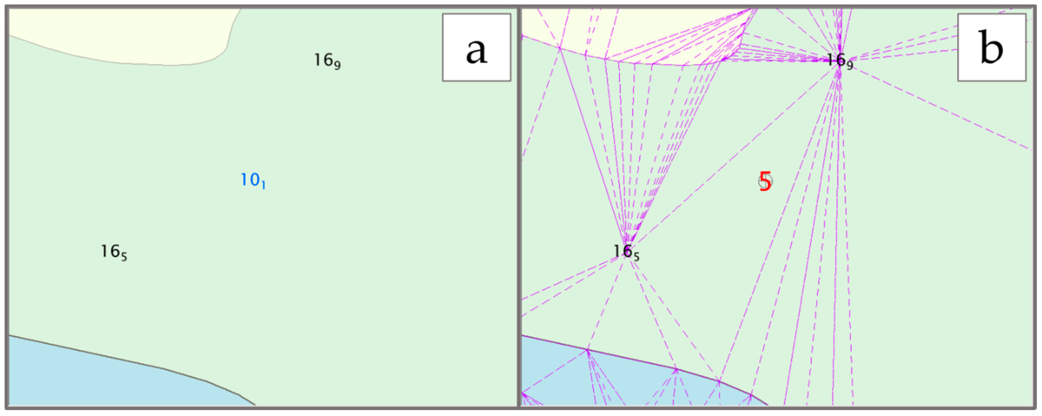
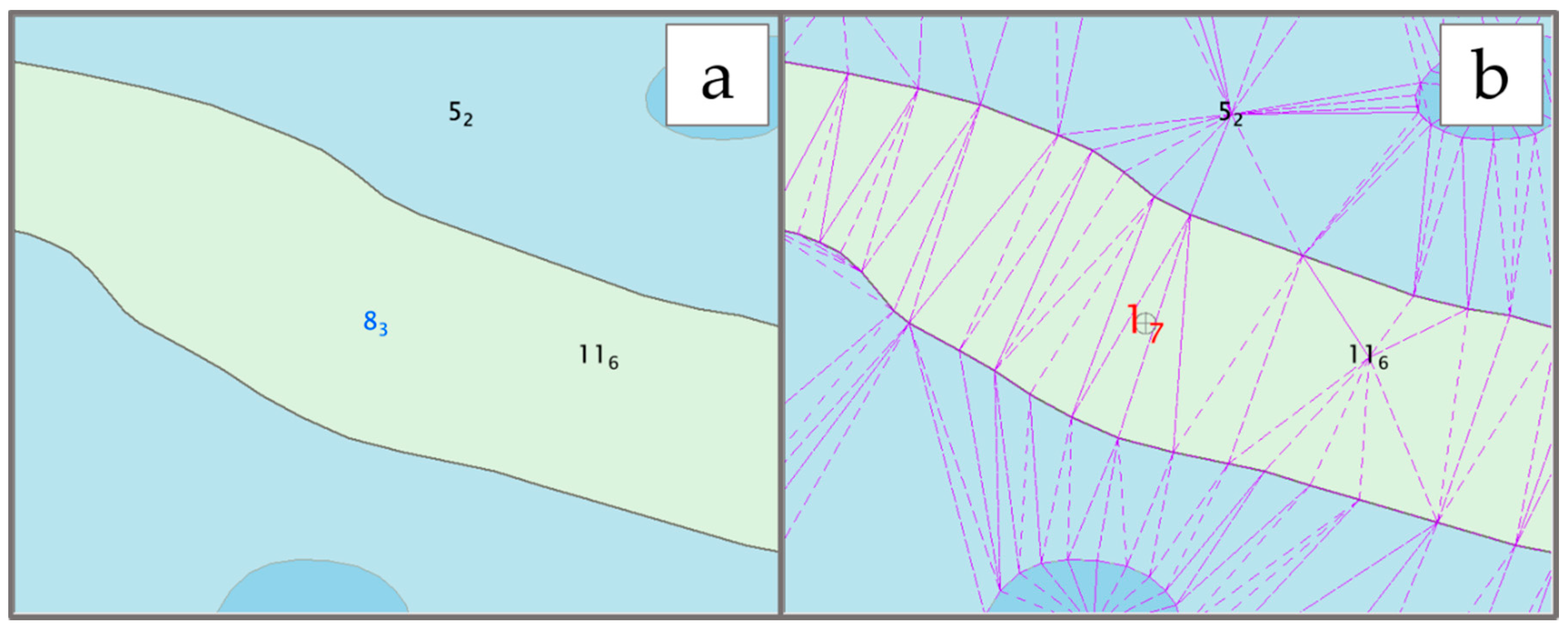
A common use case of the point-in-polygon test is provided by the mentioned possible presence of a survey sounding within a flat TIN triangle. A flat triangle can be generated as the result of the triangulation in areas locally characterized by the presence of a linear feature—like a curved depth contour—not closely surrounded by other depth-defined features, see Figure 5. In such a case, the algorithm compares the given survey sounding against the validity depth range—when available—of the underlying feature polygon (e.g., a depth area).

The S-57 ENC specifications prescribe that a cell must have the entire area with data covered, without any overlap, by a restricted group of seven area feature types, called the “skin of the earth”, see

Table 3. The S-57 ENC area feature types, with the corresponding acronym, belonging to the restricted “skin of the earth” group.

Feature Type	S-57 Acronym
Navigable depth areas	DEPARE
Dredged area	DRGARE
Floating dock	FLODOC
Permanently moored ship	HULKES
Land area	LNDARE
Pontoon	PONTON
Unsurveyed depth area	UNSARE

[32]. This characteristic of an S-57 ENC contributes towards making the sounding-in-specific-feature tests effective in reducing the number of staged untested features. Furthermore, if a survey sounding is not contained in any of the skin of the earth polygons, it is outside of the ENC data coverage and thus does not represent a chart discrepancy.

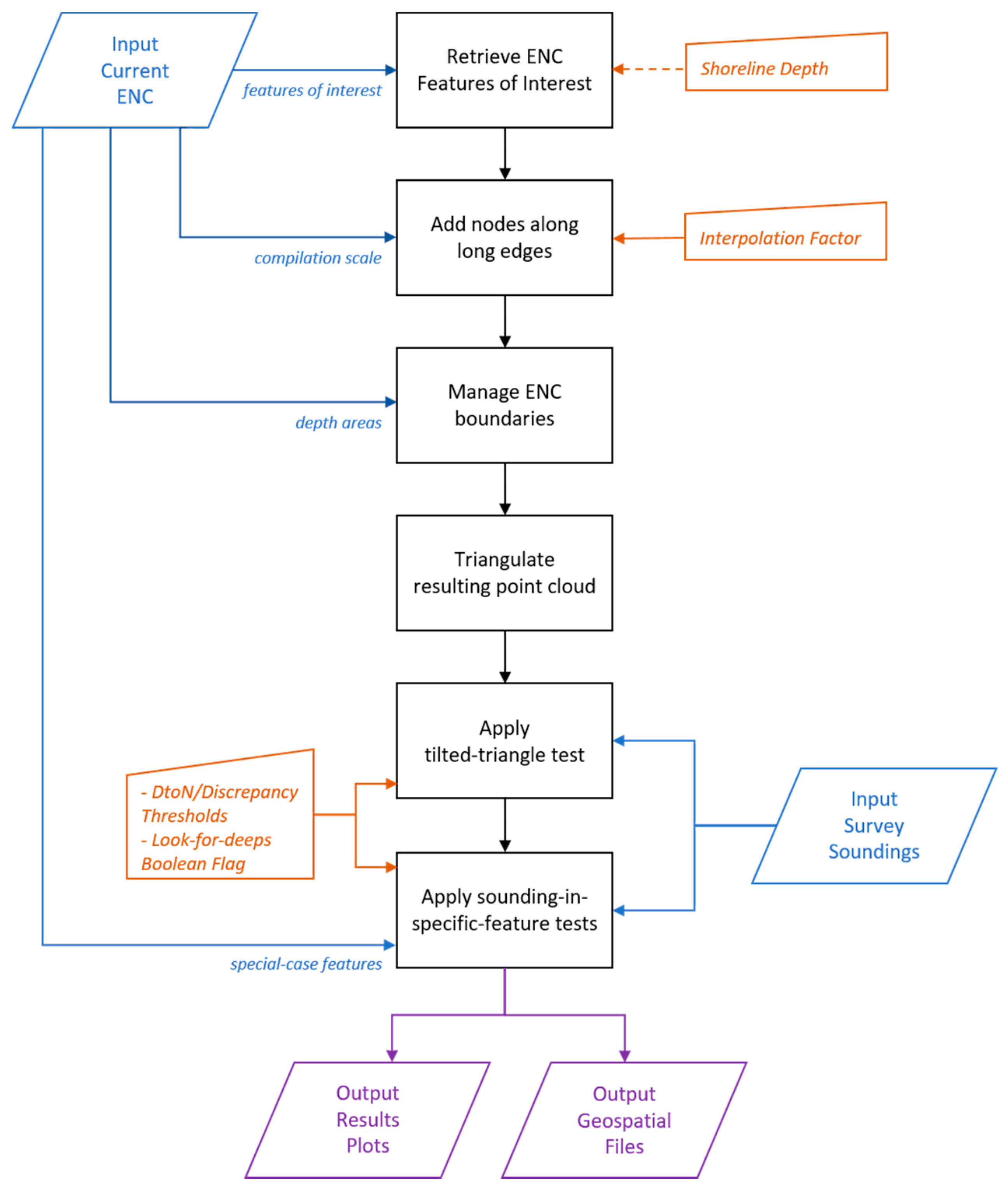
Figure 6 provides a flowchart outlining the main algorithmic steps, data inputs, user parameters, and processing outputs. The plots provided in the output should only be used for exploratory means. In fact, once the algorithm is successfully executed, the generated geospatial files should be imported in the fully-fledged GIS application of choice for results inspection and eventual application of the required modifications to the ENC.

2.6. Library Implementation, Supporting Visualization, and Output Storage

A software library (current version: 1.0) that implements the algorithm has been developed and tested mostly using the Python language (version 3.6) [47]. For a few selected profiled bottlenecks, a superset of Python, called Cython (version 0.28) [48], was used to reduce the execution time by manually adding a few static-type declarations. Using such declarations, Cython was then able to automatically convert Python code into optimized C code.

The library has been coupled with a multi-tab graphical user interface based on a Python port of the Qt framework [49]. The outcomes of the algorithm execution are visualized using the Matplotlib library [50]. ENC-derived depth values are colored by depth, while algorithm-flagged input survey soundings are colored by their discrepancy. If present, the subset of untested input soundings that require human evaluation are displayed with a magenta diamond. The default output is provided in S-57 format using internal code. For easy sorting and identification of discrepancies, the magnitude of the discrepancy against the chart is stored both as cartographic symbol features (S-57 acronym: $CSYMB) and soundings (i.e., storing the discrepancy value as the depth coordinate).

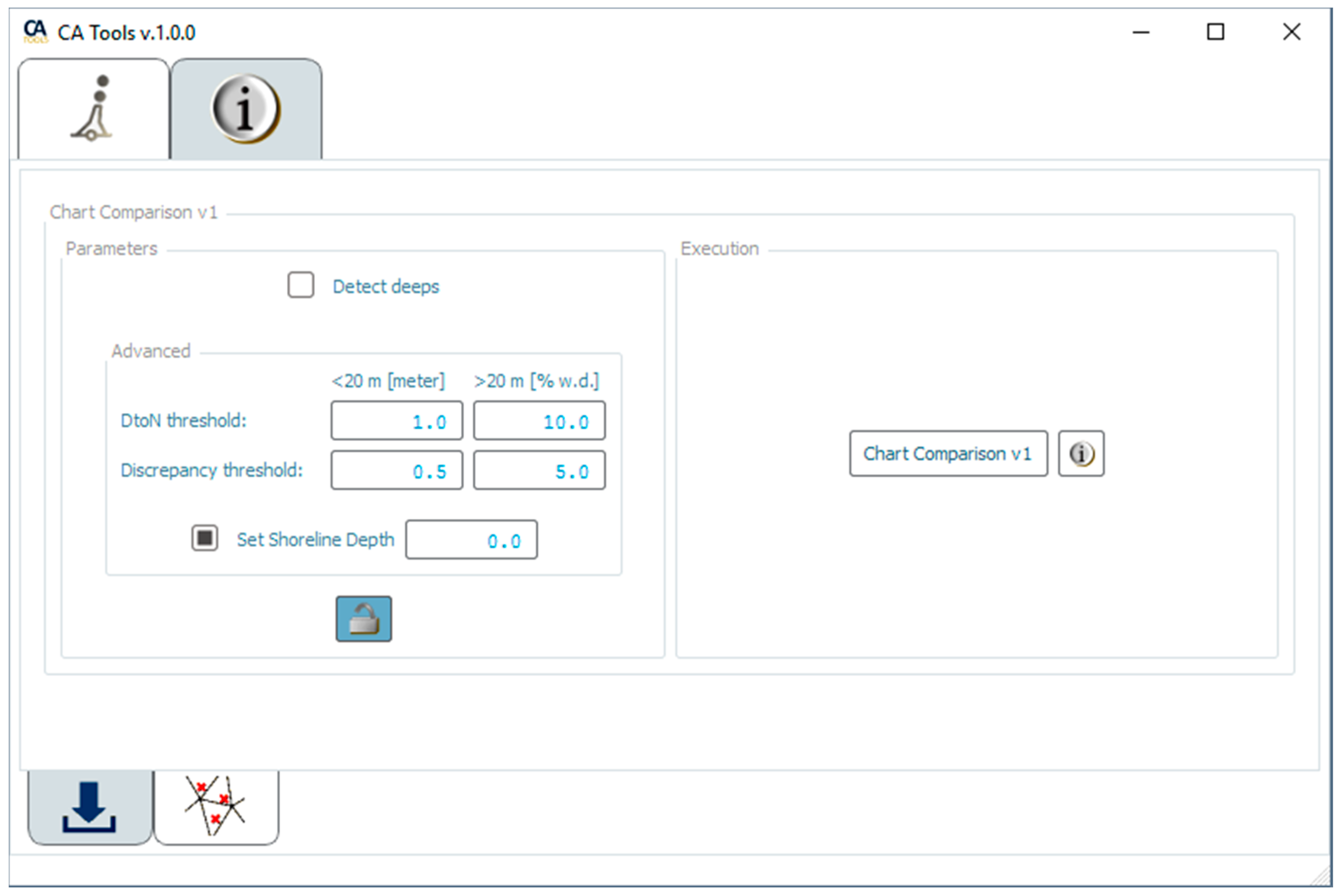
Optional output in the popular Shapefile and KML formats are generated using the Geospatial Data Abstraction Library (GDAL) package [51]. In this latter case, the TIN internally used by the algorithm is also generated for debugging aims. An implementation of the algorithm was made publicly available in the HydrOffice framework as a tab widget, see Figure 7, freely accessible in the CA Tools application (https://www.hydroffice.org/catools).

3. Results

To the best of our knowledge, the literature currently lacks algorithms specifically tailored to the identification of discrepancies between nautical charts and survey soundings and, thus, with outcomes directly comparable to the proposed algorithm. However, the algorithm results were quantitatively compared, only for the DtoNs component, with the output of a tool named DtoN Scanner (version 2) described in [25] and publicly available as part of the HydrOffice QC Tools application (https://www.hydroffice.org/qctools/main). All the algorithm results were also validated based on expert opinion.

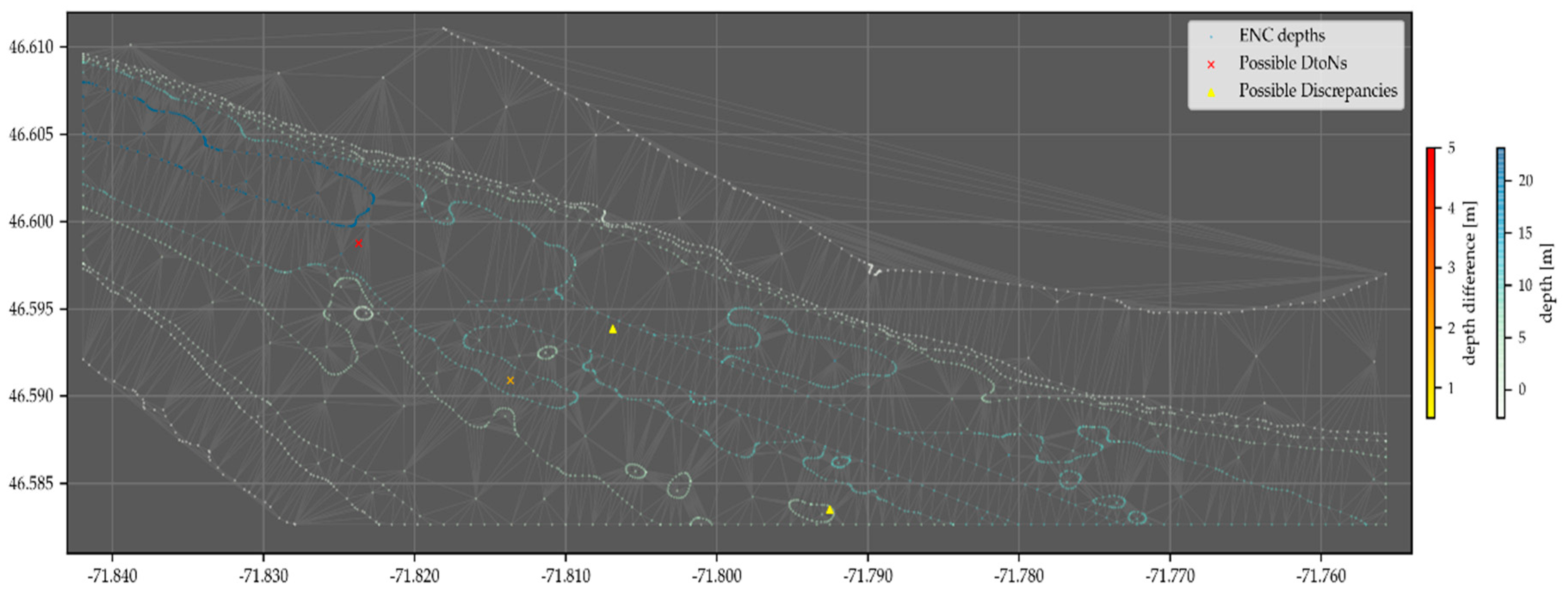
During the initial development, ad-hoc input survey soundings have been generated with two DtoNs and two chart discrepancies to be tested against a valid ENC. Using the described default settings, the algorithm was able to identify both the DtoNs and the chart discrepancies, see Figure 8.

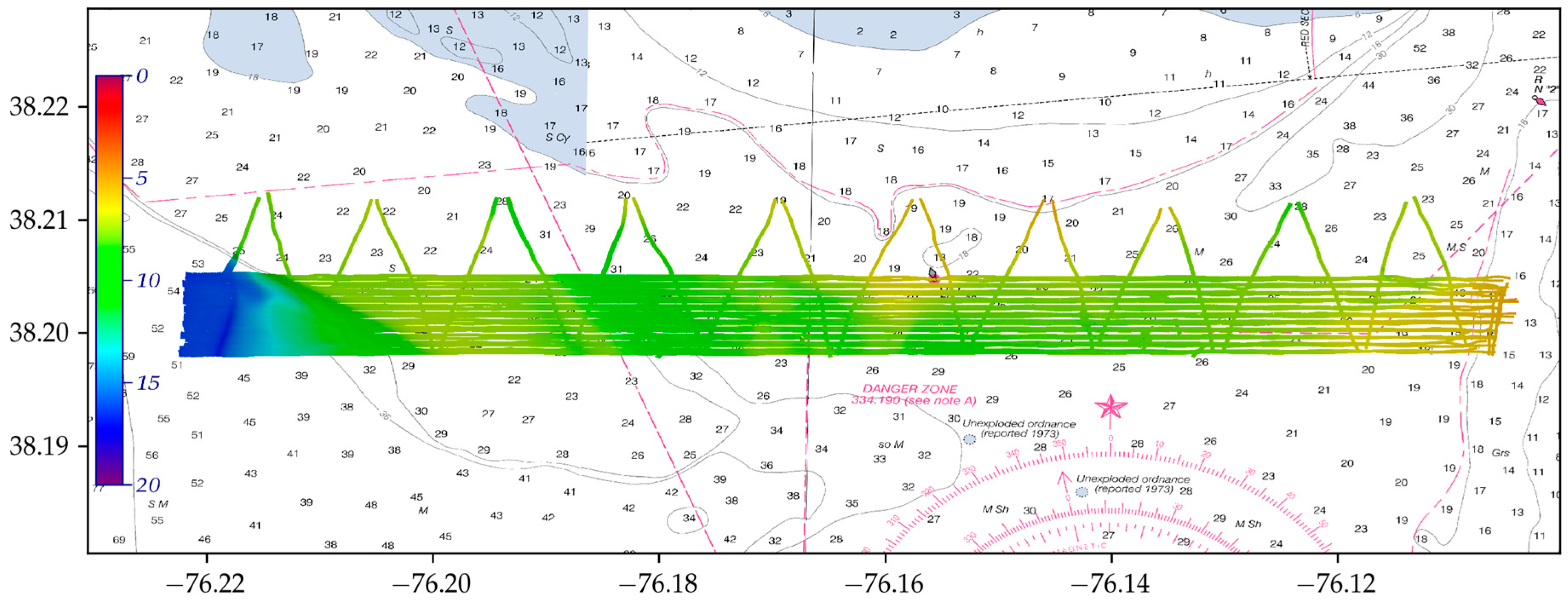
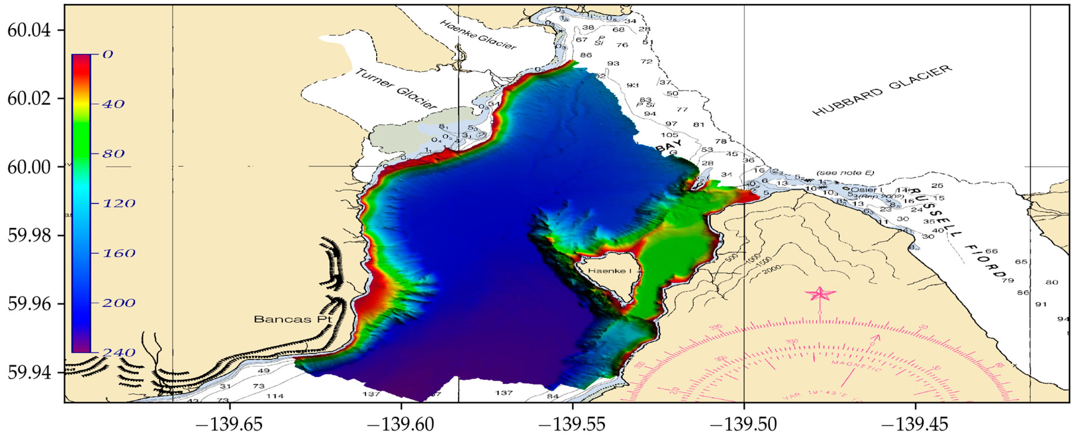
The algorithm has then been tested in several real-data scenarios using official ENCs and MBES-based survey datasets. To keep this section concise, only two of those scenarios are presented here. On one side, the analysis of the soundings from NOAA survey H12990, see Figure 9, shows relatively minor changes to the current ENCs. Conversely, the presence of large active glaciers in the area is highlighted by the analysis of the NOAA H13701 dataset. Further details of the adopted inputs are provided, for the surveys, in

Table 4. Information about the NOAA surveys presented as test datasets.

Survey	Location	Year	Scale	MBES
H12990	Chesapeake Bay (USA)	2017	1:10,000	Kongsberg EM 2040
H13071	Yakutat Bay (USA)	2017	1:40,000	Kongsberg EM 710
				Kongsberg EM 2040

and, for the ENCs, in

Table 5. Information about the NOAA ENCs used to test the algorithm.

Chart	Scale	Edition	Update Number	Issue Date
US5VA21M	1:40,000	21	0	2 May 2018
US5VA22M	1:40,000	28	2	5 June 2018
US4AK3XM	1:80,000	5	0	13 February 2018

.

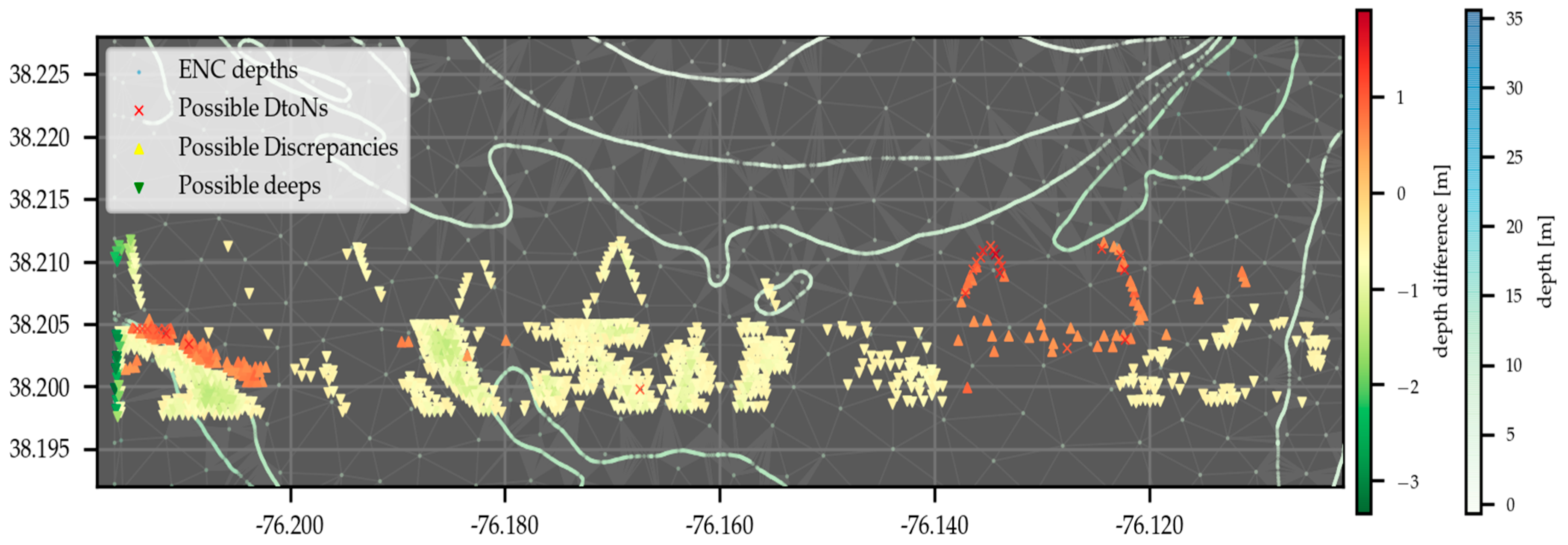
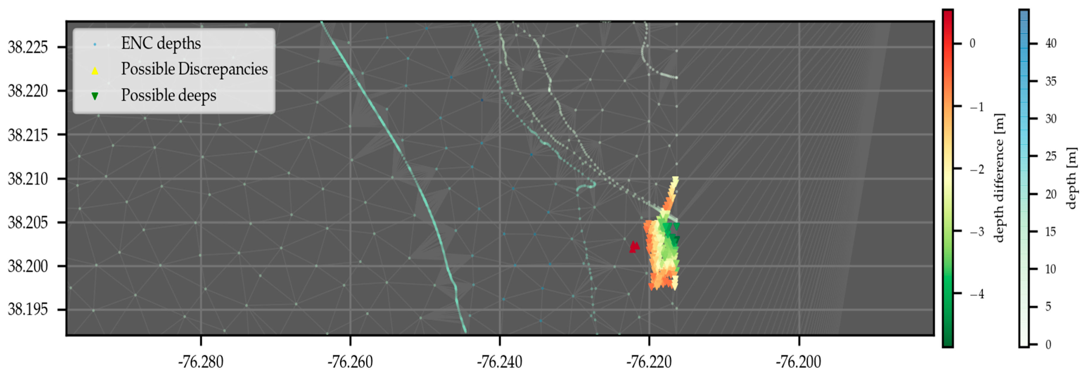
The results of the analysis for the H12990 survey dataset, see Figure 10, are shown in Figure 11 and Figure 12. These two figures represent the evaluation of the westernmost and easternmost parts, respectively, of the survey that insists on two different ENCs.

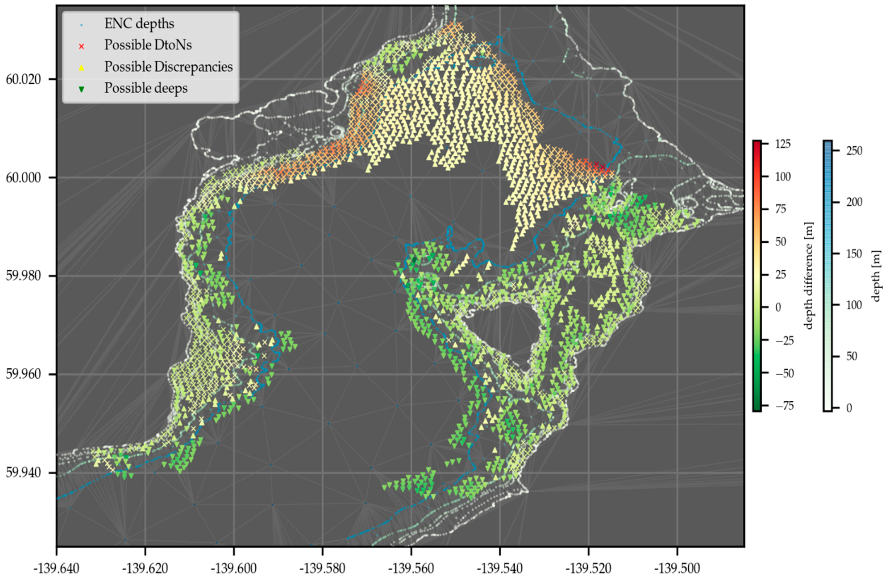
The results of the analysis for the H13701 survey dataset are shown in Figure 13.

The three applied analyses to the two presented surveys provide results that are consistent with what reported by survey analysts—using their judgment to evaluate the context surrounding the survey sounding, but with numeric criteria adherent to Table 2—after a careful but time-consuming evaluation of the same inputs, see

Table 6. Results for DtoN candidates using the proposed algorithm and the DtoN Scanner [25]. The Expert Opinion column provides the total number of DtoNs used to identify the false negatives (FN) and the false positives (FP) for the two sets of automated outputs.

Input Pair	Expert Opinion	Proposed Algorithm			DtoN Scanner
		Total	FN	FP	Total	FN	FP
Ad-hoc data pair	2	2	0	0	1	1	0
H12990, US5VA21M	25	25	0	0	23	7	5
H12990, US5VA22M	0	0	0	0	1	0	1
H13701, US4AK3XM	713	713	0	0	674	51	12

, for DtoN candidates, and

Table 7. Results for chart discrepancies using the proposed algorithm. The Expert Opinion column provides the total number of chart discrepancies used to identify the false negatives (FN) and the false positives (FP) for the automated output.

Input Pair	Expert Opinion	Proposed Algorithm
		Total	FN	FP
Ad-hoc data pair	2	2	0	0
H12990, US5VA21M	107	110	0	3
H12990, US5VA22M	2	3	0	1
H13701, US4AK3XM	779	784	0	5

, for chart discrepancies. The comparison with the expert opinion identified the presence of a few false positives, as shown in Table 7, mainly localized close to the ENC boundaries. This is not surprising given the currently adopted approach of using the minimum value in depth areas along the ENC boundaries for introducing additional nodes. A possible future improvement to mitigate such an issue is the merging of point clouds retrieved from adjacent ENCs—with the same navigational purpose—before performing the “triangulate resulting point cloud” step, see Figure 6.

For the DtoNs candidates, the proposed algorithm performed better than the DtoN Scanner in terms of both false negatives and false positives. The better performance can be reconducted to the adoption of more capable tests (the DtoN Scanner only uses a “flat” triangle test with the shallowest depth of each of the triangle vertices) and the additional techniques adopted during the construction of the point cloud from the ENC (e.g., the long-edge interpolation, the adoption of a proper shoreline depth value, the retrieval of the ENC boundaries).

4. Discussion

Although the algorithm has been successfully tested with several pairs of real-world ENCs and survey datasets, more tests are required to identify possible shortcomings and corner cases absent in the analyzed scenarios. However, the handling of eventual issues will likely happen by extending the described two-step approach and, thus, preserve the general validity of the algorithm proposed in this work.

Although popular, the IHO S-57 ENC format is not the only available format to store the geospatial vector information of a nautical chart for use with an ECDIS (e.g., the National Geospatial Agency’s Digital Nautical Chart format, the coming IHO S-101 standard) [33,52]. Although this work is based only on ENC data in the IHO S-57 format, the extension to other ENC formats should be straightforward.

The survey soundings are ultimately limited by the quality of the original observations used to sample the seafloor [53]. This consideration acquires increasing relevance when the dimensions of the measured chart discrepancies approach the limits—that should be experimentally evaluated or retrieved by the specifications declared by the manufacturer—of the sonar system used for the survey [54]. The sonar detection uncertainty represents just one potential source of artifacts with a variety of other potential environmental, integration, and datum reduction issues that can badly affect the final survey soundings [35,55]. When this happens, bathymetric artifacts generated by the acoustic imaging geometry may be mistaken as chart discrepancies. Among other institutions, the International Hydrographic Organization has developed rules and best practices for the execution of a hydrographic survey that fulfills the minimum quality requirements for charting aims [56,57]. However, the execution of a hydrographic survey is not always targeted at the production of nautical charts. New hydrographic data are collected for a variety of reasons that spans from scientific research to military applications and marine constructions [58]. Given the high cost of data collection at sea, the national hydrographic offices usually attempt to use these surveys, when available, for charting purposes. As such, a buffer representing a lower limit of what is considered a chart discrepancy should also consider an estimation of the soundings quality based on the specific survey being analyzed.

A preliminary step in the application of the algorithm consists of the retrieval of the information content present in the input ENC. Ideally, such a content should be used to reconstruct a continuous bathymetric model of the ENC’s underwater area that matches—as close as possible—the intent of the chart makers and the expectations of the chart readers. In practice, it is unlikely that, based on different precautionary principles and contingent valuations, two random navigators would draw a perfectly overlapping intermediate contour on a given ENC area. Given the complexity and inherent subjectivity involved in the bathymetric reconstruction, we opted for a simplified, still reasonable solution for the task by generating a TIN from the set of three-dimensional nodes retrieved from the chart and then assuming a linear variation of the model among those nodes.

As an alternative to the use of the Delaunay conforming triangulation, future works may explore the creation of the TIN based on a constrained Delaunay triangulation [59,60], since this technique makes it possible to explicitly define edges (“breaklines”) that are not modified by the triangulator (thus removing the currently required addition of interpolated nodes along long edges). However, the adopted point densification for long feature edges provides a controlled means to introduce nodes in the triangulation. Thus, we will likely also explore the adoption of a hybrid solution.

The conversion by interpolation of a TIN into a regular grid to perform discrepancy analysis represents quite a popular operation. However, although the several intrinsic advantages related to deal with grid data (e.g., higher processing and development speed) [36], we decided not to take such a direction because of the intrinsic variable-resolution nature of an ENC that makes it difficult to identify the best fixed resolution at which to grid the TIN. Regarding the possible creation of a variable-resolution grid, despite the recent development and successful application of this type of gridding algorithms to MBES data [61], a robust estimation of the local resolution based on ENC-derived data would have represented a challenge, and it is an open research question.

To the best of our knowledge, this work represents the first appearance in literature of a proposed algorithm for identifying discrepancies between nautical charts and survey soundings. Thus, there is a lack of research efforts that the results of this work can be directly compared with, with the notable exception of the DtoN Scanner [25]. However, the described tilted-triangle test may be seen as an evolution of a well-known best practice in nautical cartography for the representation of depth during chart compilation [21]. Such a practice, known as the “triangular method of selection” [62], is commonly used to drive the selection of the charted soundings, and it is based on the following two tests:

• Triangle test. Within a triangle of charted soundings, no survey sounding is present which is less than the shallowest depth values defining the corners of the triangle.
• Edge test. Between two adjacent charted soundings, no survey sounding exists that is shallower than the lesser of the two charted soundings.

The application of these tests presents some well-known scale- and data density-dependent issues (e.g., which spatial buffer to apply for the edge test? What is the significance of the triangle test with narrow elongated triangles?) that the tilted-triangle test potentially overcomes.

5. Conclusions

The present work provides evidence that, with respect to the chart adequacy assessment, the adoption of the described two-step algorithm brings several improvements (e.g., less subjectivity and time of execution) in comparison to the current commonly-adopted practices.

Future works will focus on exploring techniques to better reconstruct the bathymetric model from ENCs (i.e., attempting to better capture the cartographer and the mariner interpretations of the charted bathymetry) and evaluating the adaptation of the algorithm to chart compilation aims as a replacement for the triangle test and the edge test.