Duality and Dimensionality Reduction Discrete Line Generation Algorithm for a Triangular Grid

Abstract

Vectors are a key type of geospatial data, and their discretization, which involves solving the problem of generating a discrete line, is particularly important. In this study, we propose a method for constructing a discrete line mathematical model for a triangular grid based on a “weak duality” hexagonal grid, to overcome the drawbacks of existing discrete line generation algorithms for a triangular grid. First, a weak duality relationship between triangular and hexagonal grids is explored. Second, an equivalent triangular grid model is established based on the hexagonal grid, using this weak duality relationship. Third, the two-dimensional discrete line model is solved by transforming it into a one-dimensional optimal wandering path model. Finally, we design and implement the dimensionality reduction generation algorithm for a discrete line in a triangular grid. The results of our comparative experiment indicate that the proposed algorithm has a computation speed that is approximately 10 times that of similar existing algorithms; in addition, it has better fitting effectiveness. Our proposed algorithm has broad applications, and it can be used for real-time grid transformation of vector data, discrete global grid system (DGGS), and other similar applications.

1. Introduction

Vector and raster are two fundamental spatial data models, each having advantages for various applications. The process of discretizing a vector to its corresponding grid cells under certain criteria is referred to as “gridding” or “rasterization”, with this facilitating the fusion between vector and raster data. In general, vector data models abstract real-world entities into a combination of geometric elements, such as points, lines, and polygons [1]. The discretization of geometric elements therefore forms the basis of vector data discretization. For discretization of line and polygon elements, the grid path or grid boundary of the line or polygon must first be determined. Thus, the core problem of discretization is the generation of a discrete line [2,3].

In the fields of computer graphics and geographical information systems, various efficient discrete line generation algorithms have been developed. Typical examples include the digital differential analyzer (DDA) algorithm [4], the midpoint line algorithm [5], and the Bresenham algorithm [6]. Furthermore, based on the latter, Wu and Rokne proposed a double-step incremental generation algorithm [7], Jia proposed a six-step algorithm for line drawing [8], and Huang and Zhang proposed a self-adaptive step straight-line algorithm [9]. These algorithms were primarily intended for rectangular (quadrangular) grids; however, triangular and hexagonal grids are also used in many applications. It should be noted that although Vince [10] developed a mathematical model for discrete lines based on a multidimensional grid system and designed a corresponding algorithm, this model is applicable only to grid systems obtained by moving the centrosymmetric cell, such as a square, hexagon, or cube; thus, this algorithm is not suitable for a triangular grid, the cells of which are noncentrosymmetric. The triangular grid has been applied to discrete global grid system (DGGS). Representative achievements include Sphere Quad Tree [11] and Quaternary Triangular Mesh (QTM) [12], which are mainly used in spatial data indexing [13] and map generalization models [14]. Both hexagonal and diamond grids can be formed by triangular grid polymerization. During the visualization process, some typical 3D programming interfaces, such as OpenGL, provide the function to directly handle triangular grids after triangulation and striping of complex objects [15]; triangular grids are therefore useful. However, they are not uniformly adjacent; (in the case of grid cells, adjacency may be at edges, vertices, or both—if there is only edge adjacency, the grid is uniformly adjacent, otherwise it is non-uniformly adjacent). Grid cells also have different orientations (including upper and lower triangles), and the geometric structure of triangular grids is therefore quite complex, posing challenges for discrete line generation. There is also a dearth of related research. Freeman proposed a vertex-to-vertex discrete line generation algorithm that selects grid cells based on the distance between the vertex and vector line [16]; consequently, some cells of the discrete line deviate from the vector line. Nagy generated a discrete line using neighborhood sequences in a triangular grid [17]; the constraining conditions, including adjacent relationship of grid cells and length of the shortest path, are not sufficient to guarantee the uniqueness of a path. Sarkar proposed the shortest path search algorithm along the boundary of the triangular grid cell [18]; however, this algorithm ignores the relationship between the cell center and the vector line. Zhang proposed the full-path algorithm, in which, according to the geometric relationship between the vector line and grid cell, all grid cells crossed by the vector line are selected one by one [2]; the discrete line generated by this algorithm is ideal, but the process is complex, and computation speeds are slow. Dutt discussed the case in which a straight line crosses a vertex of the triangular grid cell, and based on this case, proposed a discrete line generation algorithm for a triangular grid [19]; however, the entire process needs to be conducted in a triaxial coordinate system, with the consequence that computation speeds are slow. In summary, for the generation of a discrete line in a triangular grid, there is currently no algorithm that has both satisfactory outcomes and reasonable computation speeds. We therefore propose a new algorithm in order to advance this research field.

Compared with a triangular grid, the geometric structure of a hexagonal grid is ideal, making it easy to establish the discrete line model. Based on the structural characteristics of triangular and hexagonal grids, we therefore define a new positional relationship between the two grid systems henceforth referred to as “weak duality”, which ensures maximum overlap between the centers of hexagonal and triangular grids. Based on this weak duality relationship between grid systems, we establish a mathematical model for triangular grid discrete line generation, using the hexagonal discrete line model. In addition, we solve the model using the dimensionality reduction method to theoretically simplify the problem.

2. Definition of Duality and Weak Duality

Generally speaking, a duality in mathematics translates concepts, theorems, or mathematical structures into other concepts, theorems, or structures, in a one-to-one fashion [20]. For example, the duality of the grid refers to the unique positional relationship between two different grid systems. For a regular grid, the corresponding duality grid can be obtained by connecting the centers of adjacent cells and considering them as vertices [21]. A duality relationship exists between a triangular grid and a hexagonal grid. Let the side length of the triangular grid cell be $l_t$; then, the side length of the hexagonal grid cell having a duality relationship with it is $l_h=\frac{1}{\sqrt{3}}{l}_t$, and their sides are perpendicular to each other, as shown in Figure 1.

The center of the grid cell is typically used as a reference point for calculation and location, instead of the entire grid cell [22]. To simplify the process of grid transformation, the centers of the triangular and hexagonal grid cells should therefore be as coincident as possible. It is evident that the duality relationship shown in Figure 1 cannot meet this requirement. However, by adjusting the side length of the hexagonal grid cell to $l_h^{\prime }=\frac{1}{3}{l}_t$, and letting it be parallel to the side of the triangular grid cell, the center of a hexagonal grid cell not centered at the vertex of the triangular grid coincides with that of the triangular grid cell, as shown in Figure 2. In this study, this relationship is referred to as weak duality, and it can ensure that the centers of triangular and hexagonal grid cells coincide, facilitating transformation of the grid system.

3. Discrete Line Model of a Triangular Grid

Because of the non-uniform adjacency (the grid cells of the triangular grid have both edge and vertex adjacency) and dissimilar directions of cells in a triangular grid, it is difficult to establish a discrete line model for the grid. In contrast, it is easier to establish a discrete line model in a hexagonal grid. Based on the weak duality relationship between triangular and hexagonal grids, we can simplify the discrete line model in a triangular grid by transforming the discrete line model of a hexagonal grid into that of a triangular grid.

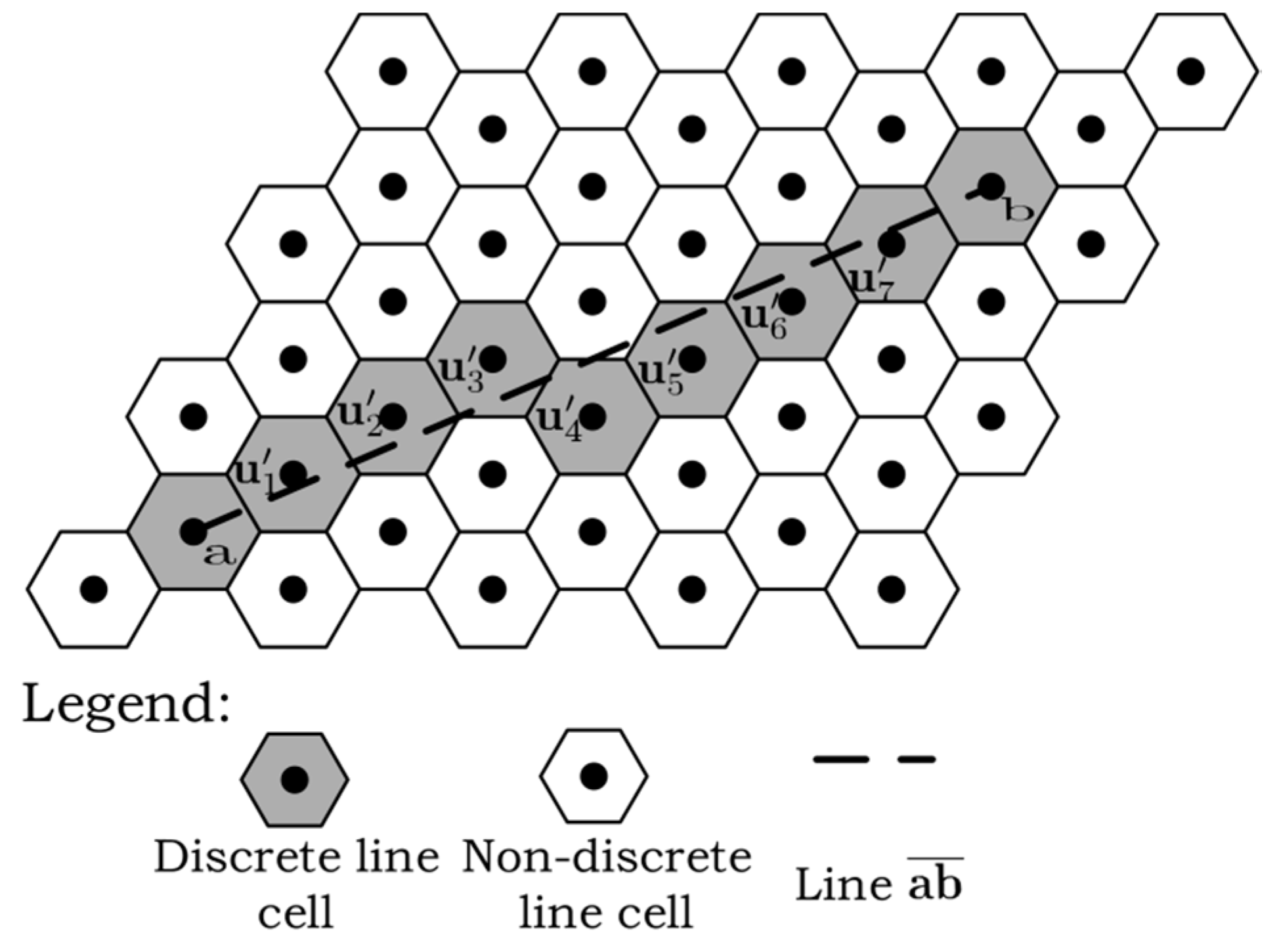
3.1. Discrete Line Model of a Hexagonal Grid

The corresponding discrete line of vector line $\overline{\mathrm{ab}}$ is a grid path that fits the vector line accurately. In a hexagonal grid, we consider a set of vectors from the center of a cell to the center of its adjacent cells as direction vectors, shown in Figure 3. Two direction vectors that are not on the same line are linearly independent, and the discrete line from the starting cell to the ending cell can be represented by the ordered sequence of any two linearly-independent direction vectors. In practice, the two direction vectors that have the smallest angle with the vector line are selected to generate the discrete line; these two direction vectors are referred to as optimal direction vectors and are denoted by $V^{\prime }=\{{\mathrm{v}}_0^{\prime },{\mathrm{v}}_1^{\prime }\}$. Then, $\overline{\mathrm{ab}}={\sum }_{{\mathrm{v}}^{\prime }\in V^{\prime }}{m}_{\mathrm{v}\prime }{\mathrm{v}}^{\prime }$, where $m_{{\mathrm{v}}^{\prime }}$ is a unique positive integer.

Let $W^{\prime }=({\mathrm{w}}_1^{\prime },{\mathrm{w}}_2^{\prime },\cdots ,{\mathrm{w}}_N^{\prime })$ be any ordered multiset of elements from $V^{\prime }$; i.e., ${\mathrm{w}}_k^{\prime }$ can be any element of $V^{\prime }$. Then, the hexagonal grid cells that form the discrete line can be expressed as ${\mathrm{u}}_k^{\prime }=\mathrm{a}+{\mathrm{w}}_1^{\prime }+{\mathrm{w}}_2^{\prime }+\cdots +{\mathrm{w}}_k^{\prime }$, while the corresponding discrete line can be denoted as $\mathrm{a}={\mathrm{u}}_1^{\prime },{\mathrm{u}}_2^{\prime },\cdots ,{\mathrm{u}}_N^{\prime }=\mathrm{b}$.

We cannot determine the unique discrete line based only on the starting and ending cells; the following constraints are therefore imposed [10]:

• There should be a minimum number of discrete line cells;
• Of all discrete lines that satisfy (1), the selected discrete line should minimize $\underset{1\le k\le N}{\max }d({\mathrm{u}}_k^{\prime },\overline{\mathrm{ab}})$, where $d({\mathrm{u}}_k^{\prime },\overline{\mathrm{ab}})$ is the vertical distance from ${\mathrm{u}}_k^{\prime }$ to $\overline{\mathrm{ab}}$.

The discrete line satisfying the constraints is unique and has the highest fitting accuracy among all discrete lines satisfying (1), as shown in Figure 4. Fitting accuracy can be described by the vertical distance between the center of the discrete line cell and the vector line. In general, the shorter the vertical distance, the higher the fitting accuracy.

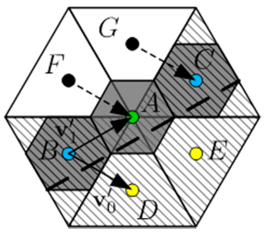
3.2. Discrete Line Model of a Weak Duality Triangular Grid

The hexagonal grid shown in Figure 4 describes the corresponding weak duality triangular grid; there is a conversion relationship between triangular and hexagonal grids. Furthermore, as shown in Figure 5, based on the weak duality relationship, the grid cells of the hexagonal discrete line are divided into two types; cells belonging to the first type are those with centers coinciding with triangular centers, shown by blue dots, while cells belonging to the second type are those with centers coinciding with triangular vertices, indicated by green dots. Let ${\mathrm{u}}_k$ represent the discrete line cells of the triangular grid, and let ${\mathrm{u}}_k^{\prime }$ represent those of the hexagonal grid. For the first cell type, ${\mathrm{u}}_k={\mathrm{u}}_k^{\prime }$; however, for the second cell type, further analysis is required.

As shown in Figure 6, the discrete line cell of the hexagonal grid ${\mathrm{u}}_A^{\prime }$, which belongs to the second cell type, has two adjacent cells, the centers of which correspond to the triangular cells, with these having the same direction. Let ${\mathrm{u}}_B^{\prime }$ be the previous cell of ${\mathrm{u}}_A^{\prime }$, and let vectors ${\mathrm{v}}_0^{\prime }$ and ${\mathrm{v}}_1^{\prime }$ be the optimal direction vectors of line $\overline{\mathrm{ab}}$, and let ${\mathrm{u}}_C$ be the corresponding triangular cell of ${\mathrm{u}}_A^{\prime }$. We can obtain the center of ${\mathrm{u}}_C$ by moving the center of ${\mathrm{u}}_B^{\prime }$ along the vector ${\mathrm{v}}_1^{\prime }$.

In contrast, as shown in Figure 7, the triangular cells to which the centers of ${\mathrm{u}}_B^{\prime }$ and ${\mathrm{u}}_C^{\prime }$ correspond have different directions. Cells ${\mathrm{u}}_D,{\mathrm{u}}_E,{\mathrm{u}}_F,$ and ${\mathrm{u}}_G$ might correspond to ${\mathrm{u}}_A^{\prime }$. By moving the centers of ${\mathrm{u}}_A^{\prime }$ and ${\mathrm{u}}_B^{\prime }$ along the vector ${\mathrm{v}}_0^{\prime }$, we can obtain the centers of ${\mathrm{u}}_D$ and ${\mathrm{u}}_E$. In a similar manner, the centers of ${\mathrm{u}}_F$ and ${\mathrm{u}}_G$ can be obtained by moving the centers of ${\mathrm{u}}_A^{\prime }$ and ${\mathrm{u}}_C^{\prime }$ along the vector $-{\mathrm{v}}_0^{\prime }$. Based on the positional relationship between the centers of ${\mathrm{u}}_A^{\prime },{\mathrm{u}}_D,{\mathrm{u}}_E,$ and line $\overline{\mathrm{ab}}$, the corresponding triangular cells of ${\mathrm{u}}_A^{\prime }$ can be determined. If the centers of ${\mathrm{u}}_A^{\prime },{\mathrm{u}}_D,{\mathrm{u}}_E$ are on different sides of the line, the corresponding triangular cells of ${\mathrm{u}}_A^{\prime }$ are ${\mathrm{u}}_D$ and ${\mathrm{u}}_E$; otherwise, the corresponding cells are ${\mathrm{u}}_F$ and ${\mathrm{u}}_G$.

Using the abovementioned corresponding relationships based on the discrete line model of a hexagonal grid and some simple manipulations, we can obtain the triangular grid discrete line of vector line $\overline{\mathrm{ab}}$, thus achieving the transformation between these two types of discrete line model.

4. Dimensionality Reduction Algorithm of the Discrete Line Model

As discussed in the previous section, the premise of obtaining the triangular grid discrete line is solving the corresponding hexagonal grid discrete line that has a weak duality relationship with the triangular grid. Given line $\overline{\mathrm{ab}}$ in a two-dimensional hexagonal grid, we can solve the discrete line using the optimal direction vectors and constraining conditions. However, it is necessary to repeatedly calculate and compare the distance from the center of the cell to the line; this reduces the computation speed of this method. By projecting the optimal direction vectors of a hexagonal grid discrete line to the straight line perpendicular to line $\overline{\mathrm{ab}}$, we can transform the discrete line formed by the ordered arrangement of the optimal direction vectors to a closed path on the one-dimensional straight line, thereby reducing dimension and computational complexity.

4.1. One-Dimensional Equivalent Form of the Hexagonal Grid Discrete Line Model

For a one-dimensional line, the two opposite vectors that originate from the origin are denoted by the set $V=\{{\mathrm{v}}_0,{\mathrm{v}}_1\}$. If there is a positive integer set $\{m_{\mathrm{v}}|\mathrm{v}\in V\}$ that makes ${\displaystyle \sum _{\mathrm{v}\in V}{m}_{\mathrm{v}}}\mathrm{v}=0$, then $V$ is considered the basic set in the one-dimensional space. Let $W=({\mathrm{w}}_1,{\mathrm{w}}_2,\cdots ,{\mathrm{w}}_N)$ be any ordered multiset of elements from set $V$, and ${\widehat{\mathrm{u}}}_k={\mathrm{w}}_1+{\mathrm{w}}_2+{\mathrm{w}}_3+\cdots +{\mathrm{w}}_k$. We can obtain a path on a one-dimensional line by connecting $0={\widehat{\mathrm{u}}}_1,{\widehat{\mathrm{u}}}_2,{\widehat{\mathrm{u}}}_3,\dots ,{\widehat{\mathrm{u}}}_N$. In addition, if ${\widehat{\mathrm{u}}}_N=0$, the path $P:(0={\widehat{\mathrm{u}}}_1,{\widehat{\mathrm{u}}}_2,{\widehat{\mathrm{u}}}_3,\dots ,{\widehat{\mathrm{u}}}_N=0)$ is a closed path. Let $w(P)=\underset{1\le k\le N}{\max }|{\widehat{\mathrm{u}}}_k|$ ($|{\widehat{\mathrm{u}}}_k|$ is the distance from ${\widehat{\mathrm{u}}}_k$ to origin) be the farthest distance that path $P$ wanders from the origin. Then, $w(V)=\min w(P)$ is the optimal wandering distance for set $V$, and the corresponding closed path is referred to as the optimal wandering path [10].

As described in Section 3.1, the ideal discrete line should satisfy the previously mentioned constraints. After determining the optimal direction vectors, the number of discrete line cells will be minimal. Furthermore, in order to obtain the vertical distance $d({\mathrm{u}}_k^{\prime },\overline{\mathrm{ab}})$, we consider a straight line $H$ that goes through the starting point $\mathrm{a}$ and is perpendicular to line $\overline{\mathrm{ab}}$; ${\mathrm{proj}}_H$ is the vertical projection operator on $H$. Because line $\overline{\mathrm{ab}}$ is perpendicular to $H$, the projections of $\mathrm{a}$ and $\mathrm{b}$ coincide, and the vertical projections of the optimal direction vector set $V^{\prime }=\{{\mathrm{v}}_0^{\prime },{\mathrm{v}}_1^{\prime }\}$ onto $H$ form the basic set $V=\{{\mathrm{v}}_0={\mathrm{proj}}_H({\mathrm{v}}_0^{\prime }),{\mathrm{v}}_1={\mathrm{proj}}_H({\mathrm{v}}_1^{\prime })\}$. In this case, ${\widehat{\mathrm{u}}}_k={\mathrm{proj}}_H({\mathrm{u}}_k^{\prime })$ and $d({\mathrm{u}}_k^{\prime },\overline{\mathrm{ab}})=|{\widehat{\mathrm{u}}}_k|$, as shown in Figure 8. Therefore, the discrete line of the two-dimensional hexagonal grid $\mathrm{a}={\mathrm{u}}_1^{\prime },{\mathrm{u}}_2^{\prime },\cdots ,{\mathrm{u}}_N^{\prime }=\mathrm{b}$ corresponds to the closed path on the one-dimensional straight line $P:(0={\widehat{\mathrm{u}}}_1,{\widehat{\mathrm{u}}}_2,{\widehat{\mathrm{u}}}_3,\dots ,{\widehat{\mathrm{u}}}_N=0)$. Hence, solving the ideal discrete line with the shortest $\underset{1\le k\le N}{\max }d({\mathrm{u}}_k^{\prime },\overline{\mathrm{ab}})$ in two-dimensional space is equivalent to solving the one-dimensional optimal wandering path that minimizes $w(P)$.

4.2. Algorithm for Solving the Discrete Line of a Triangular Grid

Based on the above analysis, it is clear that the key to determining the optimal wandering path is to minimize $w(P)=\underset{1\le k\le N}{\max }|{\widehat{\mathrm{u}}}_k|$. To achieve this objective, we adopt the greedy algorithm, i.e., the selected vector in each step ensures that the current path is closest to the origin. The greedy algorithm is heuristic, as a result of which the solutions obtained by this algorithm may only be locally optimal; however, in this study, the solution obtained by the greedy algorithm is globally optimal, as per the following deduction:

Consider that $\{{\widehat{\mathrm{u}}}_1,{\widehat{\mathrm{u}}}_2,{\widehat{\mathrm{u}}}_3,\dots ,{\widehat{\mathrm{u}}}_N\}$ is the optimal wandering path obtained by the greedy algorithm and $\{{\widehat{\mathrm{t}}}_1,{\widehat{\mathrm{t}}}_2,{\widehat{\mathrm{t}}}_3,\dots ,{\widehat{\mathrm{t}}}_N\}$ is any non-optimal wandering path. According to the greedy algorithm, each node in the optimal wandering path is closest to the origin, so $|{\widehat{\mathrm{u}}}_1|<|{\widehat{\mathrm{t}}}_1|,|{\widehat{\mathrm{u}}}_2|<|{\widehat{\mathrm{t}}}_2|,|{\widehat{\mathrm{u}}}_3|<|{\widehat{\mathrm{t}}}_3|,\dots ,|{\widehat{\mathrm{u}}}_N|<|{\widehat{\mathrm{t}}}_N|$. If we let $|{\widehat{\mathrm{u}}}_i|=\underset{1\le k\le N}{\max }|{\widehat{\mathrm{u}}}_k|$, then $|{\widehat{\mathrm{t}}}_i|>|{\widehat{\mathrm{u}}}_i|$ must be true. There are two cases for $|{\widehat{\mathrm{t}}}_i|$: the first is $|{\widehat{\mathrm{t}}}_i|=\underset{1\le k\le N}{\max }|{\widehat{\mathrm{t}}}_k|$, in which $\underset{1\le k\le N}{\max }|{\widehat{\mathrm{u}}}_k|<\underset{1\le k\le N}{\max }|{\widehat{\mathrm{t}}}_k|$; and the second is $|{\widehat{\mathrm{t}}}_i|\ne \underset{1\le k\le N}{\max }|{\widehat{\mathrm{t}}}_k|$, in which $|{\widehat{\mathrm{t}}}_j|=\underset{1\le k\le N}{\max }|{\widehat{\mathrm{t}}}_k|$, and $|{\widehat{\mathrm{t}}}_j|>|{\widehat{\mathrm{t}}}_i|$. Because $|{\widehat{\mathrm{t}}}_i|>|{\widehat{\mathrm{u}}}_i|$, $\underset{1\le k\le N}{\max }|{\widehat{\mathrm{u}}}_k|<\underset{1\le k\le N}{\max }|{\widehat{\mathrm{t}}}_k|$ is true. Therefore, according to the greedy algorithm, we can obtain the optimal wandering path, where $w(P)=\underset{1\le k\le N}{\max }|{\widehat{\mathrm{u}}}_k|$ must be the smallest of all paths. In other words, the optimal wandering path obtained by the greedy algorithm in our study is globally optimal.

The optimal direction vector set $V^{\prime }$ corresponds to the basic set $V$; by using the greedy algorithm to find the element of basic set $V$ and the corresponding element of set $V^{\prime }$ in each step, we can therefore obtain the ideal discrete line of the weak duality hexagonal grid. Finally, based on the conversion relationship between the two discrete line models, described in Section 3.2, we obtain the discrete line of the triangular grid. The flowchart for this algorithm is shown in Figure 9.

The above algorithm successfully obtains the one-dimensional optimal wandering path, the two-dimensional discrete line of the weak duality hexagonal grid, and the two-dimensional discrete line of the triangular grid. Consequently, the proposed method gradually simplifies the problem of obtaining a triangular grid discrete line, thereby considerably improving operational efficiency.

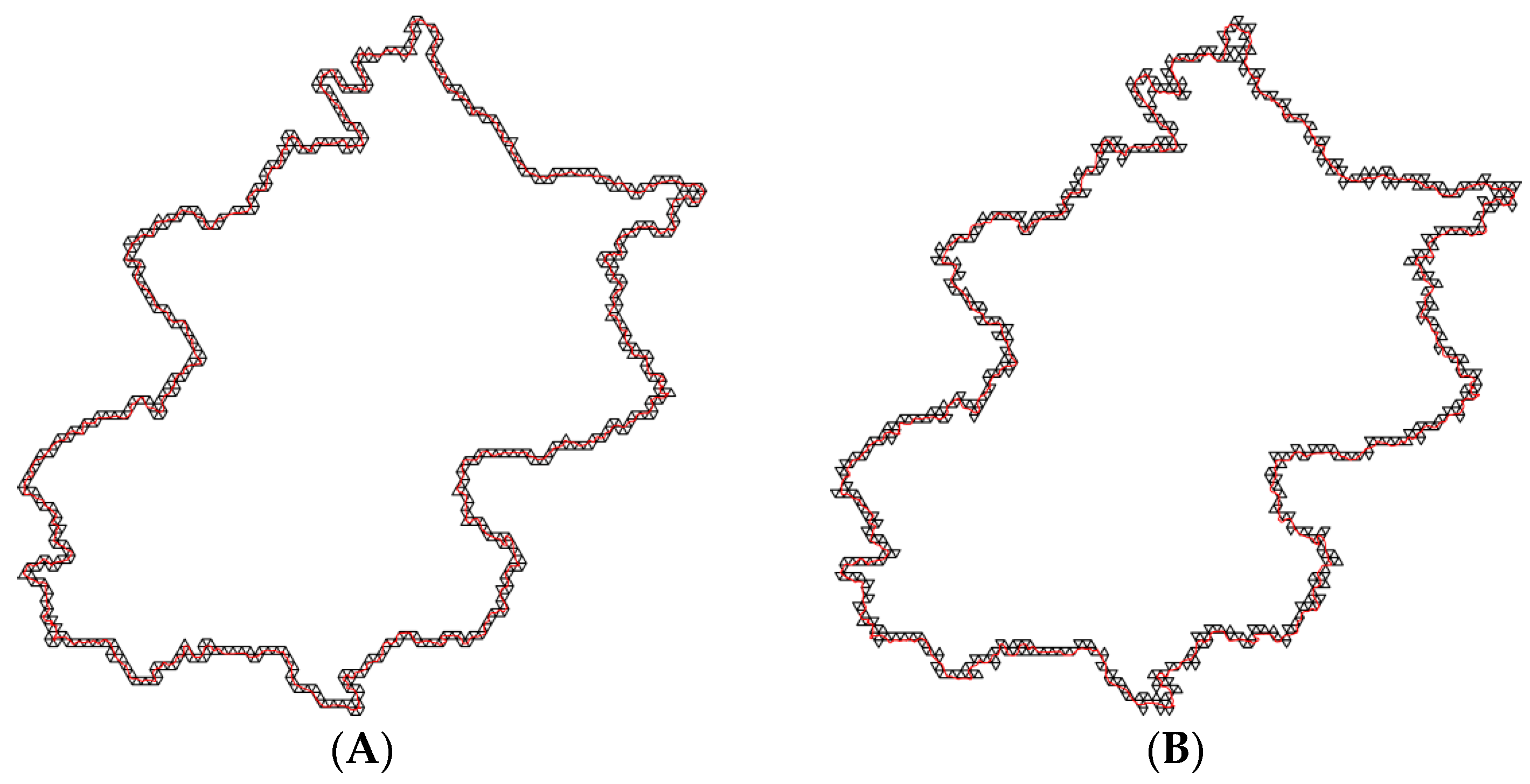
5. Experiments and Analysis

To verify the effectiveness of our proposed duality and dimensionality reduction discrete line generation algorithm, we compared it with the Freeman [16] and full-path [2] algorithms. In our study, all three algorithms were implemented in C++. Furthermore, except for the different core steps, all operations were kept the same to ensure fair and objective results. Each program was compiled into the Release version and executed on a SAMSUNG 450R5U laptop (Hardware configuration: Intel Core i5-3230M [email protected] GHz, 8 GB RAM; Operating System: Windows 7 × 64 Ultimate version; Development Tools: Visual Studio 2012). The data for the experiment were obtained from the 1:250,000 basic geographic information database of the State Bureau of Surveying and Mapping; these included the vector data of 34 provinces (municipalities directly under the central government and autonomous regions) in China, with a total of 917,264 coordinate points. Each provincial boundary was regarded as a closed polygon, and it was processed by all three algorithms.

The fitting degree between the generated discrete line and the actual vector data is an important criterion for evaluating the effectiveness of the algorithm. In practice, the closer the discrete line that is generated by the algorithm is to vector data, the higher the fitting accuracy. In this study, the average vertical distance between the center of the discrete line grid cell and the actual vector line, i.e., the ratio of the sum of the vertical distance of all discrete line cells to the total number of discrete line cells, was taken as a quantitative indicator to evaluate fitting accuracy between the discrete line and actual vector data, denoted as average distance (AVD), unit: meter (m). Generally, the smaller the AVD value, the higher the fitting accuracy of the discrete line.

When the side length of the grid cell was too large, the generated discrete line only consists of a small number of grid cells. In this case, the description of the vector boundary is very approximate and it is of no practical significance for discussing the fitting relationship between the discrete line and vector data. Therefore, in order to clearly compare the overall effectiveness and fitting accuracy of the proposed algorithm and the Freeman algorithm, we set the side length of the grid cell to 3 km and we selected Beijing for provision of test data, allowing for fewer coordinate points (3661 points). The two algorithms were used to generate discrete lines, the results of which are shown in Figure 10. According to the calculations, the AVD values of the proposed algorithm and the Freeman algorithm were 522.829 m and 1102.95 m, respectively, indicating higher accuracy of the former. The discrete lines generated by the proposed algorithm are also more continuous and smoother. Compared with the proposed algorithm, the Freeman algorithm selects discrete line grid cells based on the vertical distance between vertex and line, leading to large deviations and poor continuity and smoothness.

As shown in

Table 1. Average distance (AVD) statistical table for Freeman and proposed algorithms.

Side Length of Grid Cell (m)	Proposed Algorithm (m)	Freeman Algorithm (m)
3000	522.829	1102.95
1500	277.862	584.722
750	162.739	287.156
375	94.7479	143.333
188	49.917	68.807
94	25.473	33.800
47	12.828	17.096
23	6.292	8.253
12	3.295	4.339
6	1.650	2.152
3	0.823	1.075

, with improved grid resolution, the AVD values of both the Freeman algorithm and the proposed algorithm decrease with a reduction in grid cell side length. When the side lengths of grid cells are equal, the AVD value of the proposed algorithm is lower than that of the Freeman algorithm. This means that higher grid resolution leads to more accurate description of vector data by the discrete line, with better effectiveness using the proposed algorithm. It should be noted that no matter how high the grid resolution, even when the side length of the grid cell is reduced to 3 m, there are still deviations between the discrete line and the actual vector data, as shown in Figure 11. This is because existing discrete line generation algorithms, including the Freeman algorithm, and our proposed algorithm, all use the center or vertex of a grid cell as the reference point to generate the discrete line. However, in practice, the coordinate point of a vector is rarely at the center or vertex of the grid cell. This results in deviations between the discrete line generated by the reference point and actual vector data. This deviation is inevitable in the process of discretization, and determining ways to reduce it will be the focus of our further research.

Although the full-path and proposed algorithms produced similar results, a significant difference in computation speed was observed. As listed in

Table 2. Computation speed statistics for the full-path and proposed algorithms.

Province (Points)	Proposed Algorithm (ms)	Full-Path Algorithm (ms)	Time Ratio
Inner Mongolia (52,486)	2086.43	28,999.20	13.90
Heilongjiang (27,521)	1079.67	16,511.36	15.29
Xinjiang (37,855)	1306.59	13,895.09	10.63
Tibet (39,184)	1065.33	10,135.34	9.51
Liaoning (35,732)	676.80	4804.96	7.10
Guangdong (28,887)	689.23	5684.01	8.25
Jilin (21,588)	656.53	5563.50	8.47
Henan (21,567)	491.06	3982.95	8.11
Jiangxi (13,621)	393.64	3339.67	8.48
Hubei (19,335)	519.29	4543.93	8.75
Hainan (6065)	203.55	1640.03	8.06
Tianjin (4206)	141.69	1065.81	7.52
Beijing (3661)	144.36	1175.63	8.14
Ningxia (9704)	298.29	2423.04	8.12

(side length of grid cell is approximately 3 m), for the same data, the average computation speed of our algorithm was approximately 9.309 times that of the full-path algorithm. This is predominantly because the full-path algorithm involves sorting a large number of data points based on distance, which is highly time-consuming, whereas the proposed algorithm involves trigonometric operations only when determining the optimal direction vectors and corresponding basic set, and subsequent calculations only involve addition and subtraction because of the dimensionality reduction operation. The computational complexity of the proposed algorithm is therefore considerably lower than that of the full-path algorithm; consequently, its computation speed is higher.

6. Application of Our Algorithm in DGGS

DGGS is a promising global multiscale data model. Compared with the traditional geospatial data organization mode within a local area, DGGS is more suitable for large-scale applications, and it structurally supports efficient multi-resolution geospatial data processing [22]. Although we have thus far only discussed the application of the algorithm in the plane, the relationship between a plane and a spherical surface can be established by the icosahedron and Snyder projection. In this way, our algorithm can be extended to the spherical surface and applied to DGGS.

In the case of a set of spherical vector data, if this is inside a spherical triangle, it can be projected onto the triangular face using the forward projection (transformation from the spherical surface to the icosahedral triangular faces) of the Snyder projection. On the triangular face, the corresponding triangular grid discrete lines can be generated by our algorithm, and the discrete lines can be projected onto the spherical surface by inverse projection (transformation from the icosahedral triangular faces to the spherical surface) of the Snyder projection, thereby generating discrete lines in DGGS. However, spherical vector data is generally located at the junction of spherical triangles and will therefore be split into different spherical triangles. Following the forward projection of the Snyder projection, the triangular face corresponding to each spherical triangle has an independent coordinate system. The spherical vector data in each spherical triangle can only be processed separately, which requires solving the intersection of the spherical vector data and spherical triangle boundaries. Only in this way can the spherical vector data inside each spherical triangle be determined, and can the corresponding discrete lines be generated in DGGS by the means of the Snyder projection and our algorithm. Although we have solved the problem of the intersection of spherical vector data and spherical triangle boundaries, the specific process is more complicated and it is not the focus of this paper; we will elaborate this further in future publications.

Taking actual spherical vector data as an example, its multi-resolution display in DGGS can be achieved using our algorithm. Results are shown in Figure 12. After generating discrete lines, spatial operations such as buffer generation [23] and overlay analysis can be performed, providing a reference for solving practical problems.

7. Conclusions and Future Directions

Based on the weak duality relationship between triangular and hexagonal grids, as well as the equivalence relationship between the two-dimensional discrete line and one-dimensional optimal wandering path, we successfully performed transformations between the discrete line of a triangular grid, the discrete line of a weak duality hexagonal grid, and the optimal wandering path, thus reducing the complexity of generating a discrete line in a triangular grid.

Compared with existing algorithms, our algorithm can generate the ideal discrete line and has clear advantages in terms of computation speed. In addition, the concepts of duality and dimensionality reduction provide a new way to solve related discretization problems; our proposed method can therefore support further research.

Our proposed algorithm can be applied to real-time grid transformation of vector data, and it can also be indirectly applied to DGGS by the means of the Snyder projection and icosahedron. Meanwhile, our algorithm is beneficial for interoperation between hexagonal and triangular grids. The idea of duality and dimensionality reduction can be extended to multi-dimensional spaces; therefore, it is of great significance for the study of high-dimensionality problems, suggesting broad application prospects in the future.

References

1. Zhao, X.; Bai, J.; Wang, Z. An Adaptive Visualized Model of the Global Terrain Based on QTM. Acta Geod. Cartogr. Sin. 2007, 36, 316–320. [Google Scholar]
2. Zhang, H.; Wen, Y.; Liu, A. The Basis of Geographic Information System Algorithm; Science Press: Beijing, China, 2006. [Google Scholar]
3. Liu, R.; Li, Y. Study of Auto-vectorization Based on Scan-thinning Algorithm. Acta Geod. Cartogr. Sin. 2012, 41, 309–314. [Google Scholar]
4. Mccrea, P.G.; Baker, P.W. On Digital Differential Analyzer (DDA) Circle Generation for Computer Graphics. IEEE Comput. Soc. 1975, 100, 1109–1110. [Google Scholar] [CrossRef]
5. Reid-Green, K.S. Three Early Algorithms. IEEE Ann. Hist. Comput. 2002, 24, 10–13. [Google Scholar] [CrossRef]
6. Bresenham, J.E. Algorithm for Computer Control of a Digital Plotter. IBM Syst. J. 1965, 4, 25–30. [Google Scholar] [CrossRef]
7. Wu, X.; Rokne, J.G. Double-step Incremental Generation of Lines and Circles. Comput. Vis. Graph. Image Process. 1987, 37, 331–344. [Google Scholar] [CrossRef]
8. Jia, Y.; Zhang, H.; Jing, Y.; Liu, J. A Six-step Algorithm for Line Drawing. J. Shandong Univ. 2007, 37, 61–64. [Google Scholar]
9. Huang, B.; Zhang, L. Self-adaptive Step Straight-line Algorithms. J. Tsinghua Univ. 2006, 46, 1719–1722. [Google Scholar]
10. Vince, A. Discrete Lines and Wandering Paths. Siam J. Discret. Math. 2007, 21, 647–661. [Google Scholar] [CrossRef] [Green Version]
11. Fekete, G.; Treinish, L.A. Sphere Quadtrees: A New Data Structure to Support the Visualization of Spherically Distributed Data. In Proceedings of SPIE—The International Society for Optical Engineerin; SPIE Digital Library: Bellingham, WA, USA; Washington, DC, USA, 1990; Volume 1259. [Google Scholar] [CrossRef]
12. Dutton, G. A Hierarchical Coordinate System for Geoprocessing and Cartograph; Springer: Berlin, Germany, 1999; Volume 79. [Google Scholar]
13. Bartholdi, J.; Goldsman, P. Continuous Indexing of Hierarchical Subdivision of the Global. Int. J. Geogr. Inf. Sci. 2001, 15, 489–522. [Google Scholar] [CrossRef]
14. Dutton, G. Digital Map Generalization Using a Hierarchical Coordinate System. In Proceedings of the Automated Cartography 13, Seattle, WA, USA, 7–10 April 1997. [Google Scholar]
15. Shreiner, D.; Woo, M.; Neider, J.; Davis, T. OpenGL Programming Guide: The Official Guide to Learning OpenGL, 5th ed.; Version 2; Xu, B., Translator; China Machine Press: Beijing, China, 2006; pp. 324–341. [Google Scholar]
16. Freeman, H. Algorithm for Generating a Digital Straight Line on a Triangular Grid. IEEE Comput. Soc. 1979, 28, 150–152. [Google Scholar] [CrossRef]
17. Nagy, B.N. Shortest Paths in Triangular Grids with Neighbourhood Sequences. J. Comput. Inf. Technol. 2003, 11, 55–60. [Google Scholar] [CrossRef]
18. Sarkar, A.; Biswas, A.; Mondal, S.; Dutt, M. Finding Shortest Triangular Path in a Digital Object. In Discrete Geometry for Computer Imagery; Springer: Cham, Switzerland, 2016; pp. 206–218. [Google Scholar]
19. Dutt, M.; Andres, E.; Skapin, G.L. Characterization and Generation of Straight Line Segments on Triangular Cell Grid. Pattern Recognit. Lett. 2018, 103, 68–74. [Google Scholar] [CrossRef]
20. Maurin, K. Duality (polarity) in Mathematics, Physics and Philosophy. Rep. Math. Phys. 1988, 25, 357–388. [Google Scholar] [CrossRef]
21. Mahdavi-Amiri, A.; Harrison, E.; Samavati, F. Hierarchical grid conversion. Comput. Aided Des. 2016, 79, 12–26. [Google Scholar] [CrossRef] [Green Version]
22. Zhou, C.; Ou, Y.; Ma, T. Progresses of Geographical Grid Systems Researches. Prog. Geogr. 2009, 28, 657–662. [Google Scholar]
23. Alderson, T.; Mahdavi-Amiri, A.; Samavati, F. Offsetting spherical curves in vector and raster form. Vis. Comput. 2018, 8, 973–984. [Google Scholar] [CrossRef]
Figure 1. Duality relationship between hexagonal and triangular grids.
Ijgi 07 00391 g001
Figure 2. Weak duality relationship between hexagonal and triangular grids.
Ijgi 07 00391 g002
Figure 3. Direction vectors of a hexagonal grid.
Ijgi 07 00391 g003
Figure 4. Discrete line in a hexagonal grid.
Ijgi 07 00391 g004
Figure 5. Corresponding relationship between two discrete line models.
Ijgi 07 00391 g005
Figure 6. The triangles to which the blue dots correspond have the same direction.
Ijgi 07 00391 g006
Figure 7. The triangles to which the blue dots correspond have different directions.
Ijgi 07 00391 g007
Figure 8. Schematic of the projection relationship.
Ijgi 07 00391 g008
Figure 9. Flowchart of the duality and dimensionality reduction algorithm.
Ijgi 07 00391 g009
Figure 10. Comparison of the overall effectiveness of the two algorithms (side length of grid cells is approximately 3 km): (A) discrete line of Beijing boundary generated by the proposed algorithm and (B) discrete line of Beijing boundary generated by the Freeman algorithm.
Ijgi 07 00391 g010
Figure 11. Detailed results of the proposed algorithm (side length of grid cell is approximately 3 m), indicating the fitting relationship between the discrete line and actual vector data (A) for an inclined line; (B) at a corner; and (C) for a vertical line.
Ijgi 07 00391 g011
Figure 12. Multiresolution discretization of spherical vector data. The white arcs are the boundaries of the spherical triangles, and the figures represent the following: (A) the side length of grid cell is approximately 483 km; (B) the side length of grid cell is approximately 242 km; (C) the side length of grid cell is approximately 121 km.
Ijgi 07 00391 g012