High-Resolution Remote Sensing Data Classification over Urban Areas Using Random Forest Ensemble and Fully Connected Conditional Random Field

Abstract

As an intermediate step between raw remote sensing data and digital maps, remote sensing data classification has been a challenging and long-standing problem in the remote sensing research community. In this work, an automated and effective supervised classification framework is presented for classifying high-resolution remote sensing data. Specifically, the presented method proceeds in three main stages: feature extraction, classification, and classified result refinement. In the feature extraction stage, both multispectral images and 3D geometry data are used, which utilizes the complementary information from multisource data. In the classification stage, to tackle the problems associated with too many training samples and take full advantage of the information in the large-scale dataset, a random forest (RF) ensemble learning strategy is proposed by combining several RF classifiers together. Finally, an improved fully connected conditional random field (FCCRF) graph model is employed to derive the contextual information to refine the classification results. Experiments on the ISPRS Semantic Labeling Contest dataset show that the presented 3-stage method achieves 86.9% overall accuracy, which is a new state-of-the-art non-CNN (convolutional neural networks)-based classification method.

1. Introduction

As one of the most challenging and important problems in the remote sensing community, high-resolution remote sensing data classification is very useful for many applications such as geographical database construction, digital map updating, 3D building reconstruction, land cover mapping and change detection. The objective of this kind of classification task is to assign an object class to each spatial position recorded by the given data. Although many different algorithms have been proposed in the past, many of the problems related to the classification task have not been solved [1]. Based on different criteria, the existing classification methods can be categorized into several groups. A brief review of these existing methods is provided in the following.

According to the types of data sources employed, the existing methods can be categorized into image-based classification, 3D point cloud-based classification and data fusion-based classification. Image-based classification only makes use of the available multispectral or hyperspectral image as the sole data source in the classification, as done in previous studies [2,3]. Three dimensional points acquired by light detection and ranging (LIDAR) and dense image matching techniques [4,5] are other effective data sources for classification. For example, Vosselman [6] used high-density point clouds of urban scenes to identify buildings, vegetation, vehicles, the ground, and water. Zhang et al. [7] used the geometry, radiometry, topology and echo characteristics of airborne LIDAR point cloud to perform an object-based classification. To exploit the complementary characteristics of multisource data, data fusion based methods are also popular and have been proven to be more reliable than the single-source data methods used by many researchers [8]. For example, both images and 3D geometry data have been used in several previous studies [9,10,11,12].

In terms of the basic element employed in the classification process, the existing methods can be categorized as object-based and pixel/point-based. Object-based methods typically use a cascade of bottom-up data segmentation and regional classification, which makes the system commit to potential errors from the front-end segmentation system [13]. For instance, Gerke [14] first segmented an image into small super-pixels and then extracted the features of each super-pixel to input to an AdaBoost classifier. Zhang et al. [7] first grouped points into segments using a surface growing algorithm then classified the segments using a support vector machine (SVM) classifier. Pixel/point-based methods leave out the segmentation process and directly classify each pixel or point. However, due to the lack of contextual information, the classified results usually seem noisy. As a remedial measure, a conditional random field (CRF) is usually used to smooth the classification result. For example, both Marmanis et al. [15] and Paisitkriangkrai et al. [1] used deep convolutional neural networks (CNN) to classify each pixel, then used a CRF to refine the results, whereas Niemeyer et al. [16] first classified each 3D point using a random forest (RF) classifier then smoothed them using a CRF.

Based on the classifiers used, the existing methods can be divided into two types: unsupervised and supervised. For the unsupervised methods, expert knowledge of each class is usually summarized and used to classify the data into different categories. For instance, a rule-based hierarchical classification scheme that utilizes spectral, geometry and topology knowledge of different classes was used by both Rau et al. [9] and Speldekamp et al. [17] to classify different data. For the supervised methods, samples with labeled ground truth data are first used to train a statistical classifier (e.g., AdaBoost, SVM and RF), then the samples without labels are classified by this learned classifier. Previously, samples from small areas have been used to train the classifier, and the features of these samples have all been designed manually [7,16,18]. More recently, with the progress of sensor technology, an increasing amount of high quality remote sensing data are available for research. At the same time, progress in graphic processing unit (GPU) and parallel computing technology has significantly increased the computing capability, such that learning a more complicated classifier with a larger amount of training data has becomes accessible to more researchers. Specifically, one of the most successful practices in this direction was the launch of deep CNN (convolutional neural networks) [19,20,21,22] in the computer vision community, which has become the dominant method for visual recognition and semantic classification [13,23,24,25,26]. Furthermore, one of the most distinct characteristics of CNN is its ability to automatically learn the most suitable features, which has made the manual feature extraction process that is used in the traditional supervised-based classification methods unnecessary. Although there exists great differences between the data used in the computer vision community and the data used in the remote sensing community, some researchers [1,27] have found that the CNN models trained by the computer vision community generalize the remote sensing data and some of the features learned by the models were more discriminative than the hand-crafted features.

To promote the scientific progress of remote sensing data classification, the international society for photogrammetry and remote sensing (ISPRS) launched a semantic labeling benchmark [28] in 2014. Using the datasets provided by the benchmark, different classification methods can be evaluated and compared conveniently. We have observed an interesting phenomenon from these evaluated classification methods. On the one hand, the performances of the CNN-based methods are generally better than the non-CNN-based methods. On the other hand, the non-CNN-based methods generally use fewer training samples than the CNN-based methods. As a result, we want to explore whether the notable gap between the non-CNN and CNN-based methods can be reduced by training a traditional supervised classifier with a larger training dataset.

It is widely known that for CNN-based methods, more benefits are gained when more training data are available. However, too many training samples may lead to disaster for some traditional supervised classifiers. For example, SVMs trained by a large-scale dataset often suffer from large memory storage requirements and extensive time consumption, since an SVM solves a complex dual quadratic optimization problem [29]. In addition, the existence of too many support vectors makes the solving process extremely slow [30]. Although the RF and AdaBoost classifiers can theoretically handle a large-scale dataset, the large memory storage and computational load still hamper their applications to big training datasets. To tackle this problem and take full advantage of the information in the large-scale dataset, an RF-based ensemble learning strategy is proposed by combining several RF classifiers together in the present study. Ensemble learning or a multiple classifier system (MCS) is well established in remote sensing and has shown great potential to improve the accuracy and reliability of remote sensing data classification over the last two decades [31,32,33]. For example, Waske et al. [34] fused two SVM classifiers to classify both optical imagery and synthetic aperture radar data, and each data source was treated separately and classified by an independent SVM. Experiments have shown that their fusion method outperforms many approaches and significantly improves the results of a single SVM that was trained on the whole multisource dataset. Ceamanos et al. [35] designed a classifier ensemble to classify hyperspectral data. Spectral bands of the hyperspectral image were first divided into several subgroups according to their similarities. Then, each group was used to train an individual SVM classifier. Finally, an additional SVM classifier was used to combine these classifiers together. The results also demonstrated the effectiveness of their model fusion scheme. Recently, several fusion methods have investigated the dependence among detectors or classifiers. For example, Vergara et al. 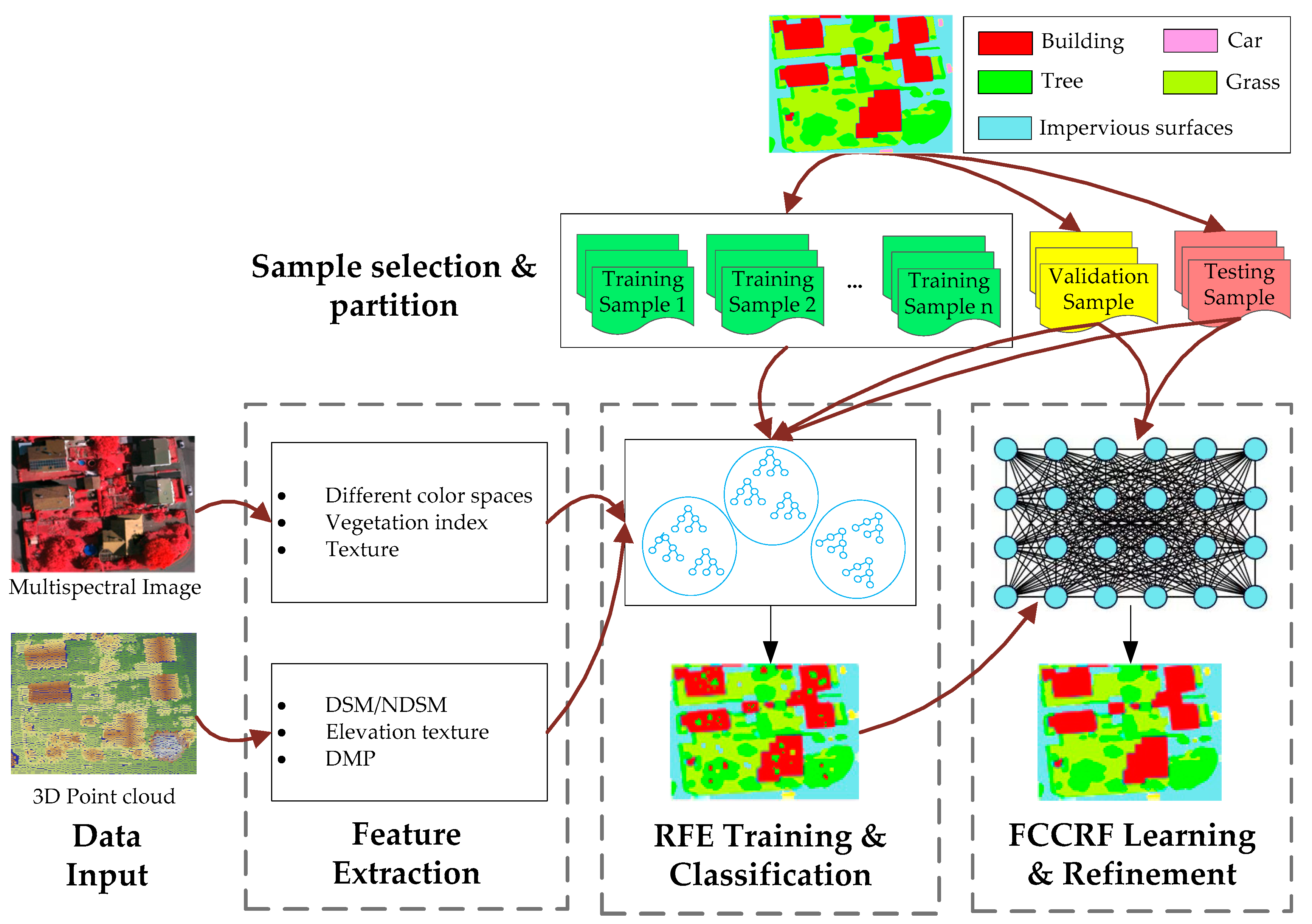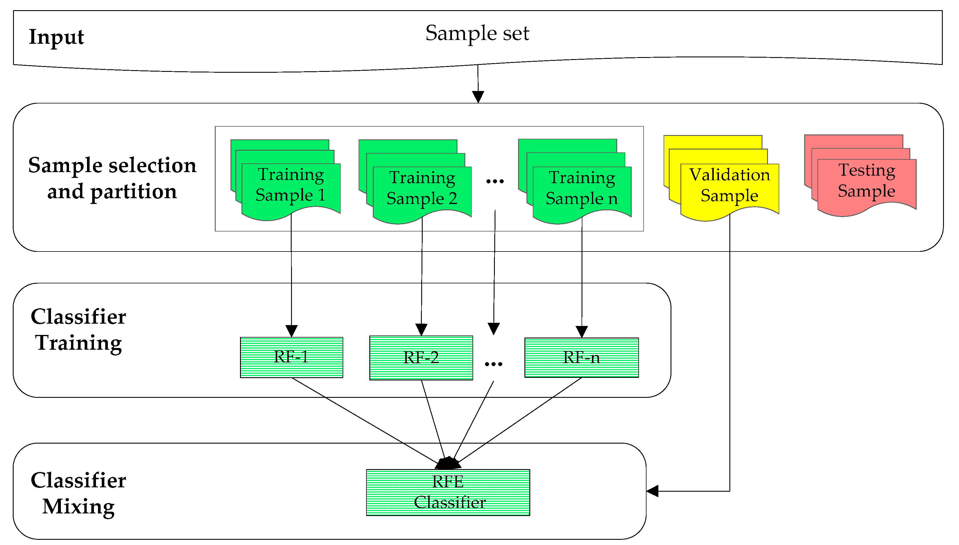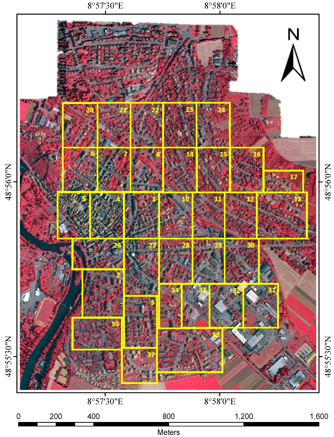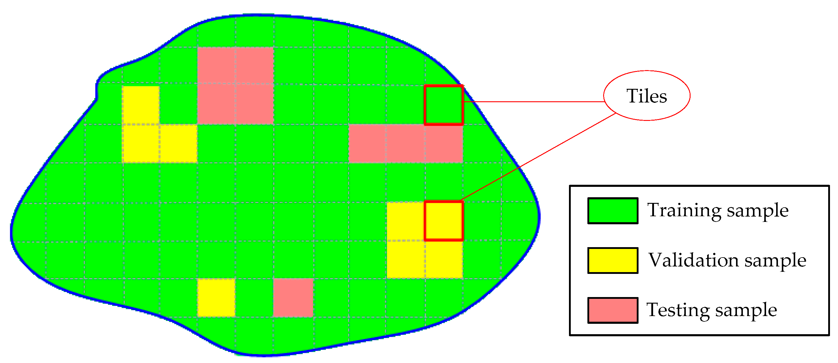[36] derived the optimum fusion rule of N non-independent detectors in terms of the individual probabilities of detection and false alarms and defined the dependence factors. This could be a future line of research in the remote sensing community. In the present study, remote sensing data (both multispectral images and 3D geometry data) are first divided into tiles. Then, some of them are selected and labeled by a human operator. After that, each selected and labeled tile is used to train an individual RF model. Finally, a Bayesian weighted average method [31] is employed to combine these individual RF models into a global classifier. In addition, to take full advantage of the contextual information in the data, an effective fully connected conditional random field (FCCRF) model is constructed and optimized to refine the classified results.

In general, the present study describes a pixel-based, supervised and data fusion-based method. The main contributions of the current study are three-fold. First, a new RF ensemble learning strategy is introduced to explore the information in the large-scale training dataset. Second, through utilizing the contextual information, an improved FCCRF graph model is designed to refine the classification result. Third, an efficient pipeline is designed and parallelized to classify the multisource remote sensing data. By testing the method on the ISPRS Semantic Labeling Contest, we achieved the highest overall accuracy among the non-CNN-based methods, which provides a state-of-the-art method and reduces the gap between the non-CNN and CNN-based methods.

The rest of this paper is organized as follows. In Section 2, details of the presented high-resolution remote sensing data classification method are elaborated. Then, experimental evaluation and analysis are reported in Section 3, and followed by some concluding remarks and future work in Section 4.

2. Methodology

The present study is composed of three main parts. First, both the high-resolution multispectral image and the 3D geometry data are used for feature extraction, and a total of 24 different features are extracted from each pixel. Second, using these pixels (samples), an RF ensemble model (constructed by combining several individual RF models; denoted by RFE) is trained and used to classify the scene. Finally, the noisy classification results are input into a learned FCCRF model, and a long-range dependencies inference is used to refine the classification results. Figure 1 shows the pipeline of the proposed method.

2.1. Feature Extraction

Four types of features are employed in this work, spectral features from the multispectral image, texture features from the multispectral image, height-related features from the 3D geometry data and differential morphological profile features from the 3D geometry data.

2.1.1. Spectral Features

The spectral features used in this paper refer to two types, the features in different color spaces and the vegetation index. They are defined as follows.

(1)

Features in different color spaces. Because each color space has its advantages, the HSV [37] and CIE Lab [38] color spaces commonly used in computer graphics and computer vision are employed in addition to the original RGB color space to provide additional information. The HSV color space decomposes colors into their hue, saturation and value components and is a more natural way to describe colors. The CIE Lab color space is designed to approximate human vision. The CIE Lab aspires to achieve perceptual uniformity and is handy to measure the distance of a given color to another color. In Section 3, we will see that both the HSV and CIE Lab are the more effective color spaces to classify remote sensing data compared to the original RGB color space.

(2)

Vegetation index. To discriminate vegetation from other classes effectively, one of the most popular vegetation indices in remote sensing, the Normalized Difference Vegetation Index (NDVI) defined as $NDVI=\raisebox{1ex}{$IR-R$}\!\left/ \!\raisebox{-1ex}{$IR+R$}\right.$, is considered. NDVI is based on the fact that green vegetation has low reflectance in the red (R) spectrum due to chlorophyll and much higher reflectance in the infrared (IR) spectrum because of its cell structure.

2.1.2. Image Texture Features

Image texture can quantify the intuitive qualities in terms of rough, smooth, silky, or bumpy as a function of the spatial variation in the pixel intensities. The effectiveness of using image texture features for remote sensing data classification has been justified by several studies [39,40,41]. Similar to [42], the following image texture features are calculated in this work:

(1)

Local range $f_{range}$ represents the range value (the maximum value minus the minimum value) of the neighborhood centered at the pixel. In areas with a smooth texture, the range value will be small; in areas with a rough texture, the range value will be larger.

(2)

Local standard deviation $f_{std}$ corresponds to the standard deviation of the neighborhood centered at the pixel. It can describe the degree of variability of a certain region.

(3)

Local entropy $f_{entr}=-{\displaystyle \sum _{i=1}^n{p}_i\log }(p_i)$, where $p_i(i=1,2,...,n)$ represents the statistics of the local histogram distribution, measures the entropy value of the neighborhood centered at the pixel. It indicates the randomness of a certain region.

When computing the three image texture features, as done in [43], the multispectral color images are first converted to gray images, and then a 3-by-3 neighborhood centered at each pixel is used for the $f_{std}$ and $f_{range}$ calculations, and a 9-by-9 neighborhood is used for the $f_{entr}$ computation.

2.1.3. Height Related Features

The height related features can be divided into two types: height features and height-based texture features. They are detailed as follows.

(1)

Height features. The corresponding digital surface model (DSM) value and the normalized digital surface model (NDSM) value for each pixel are directly used as the height features. The NDSM is defined as the difference between the DSM and the derived DEM, which describes an object’s height above the ground and can be used to distinguish the high object classes from the low object classes. Note that the height features are also used in [1,14,17].

(2)

Height-based texture features. The height-based texture features or the elevation texture features used in this study are similar to the image texture features calculated in Section 2.1.2. The features include the local geometry range feature $f_{range}^g$, the local geometry standard deviation feature $f_{std}^g$ and the local geometry entropy feature $f_{entr}^g$. In this study, we calculate these features from the DSM.

2.1.4. Differential Morphological Profile Features

Morphological profile (MP) or differential morphological profile (DMP) is an effective feature extraction method that is usually used for image classification in remote sensing [3,44]. It is used to extract the shape and size of objects based on morphological operations (e.g., opening and closing) by reconstruction. As illustrated in Figure 2, for a certain image $I$, let ${\gamma }_k^{*}$ and ${\eta }_k^{*}$ be the morphological opening and closing operators with structuring element $S{E}_k$, then $\prod \gamma (x)$ and $\prod \eta (x)$ are the opening and closing profiles at pixel $x$ of image $I$, which can be obtained by Equations (1) and (2), respectively.

$$\prod \gamma (x)=\{\prod {\gamma }_k:\prod {\gamma }_k={\gamma }_k^{*}(x),\forall k\in [0,n]\},$$

(1)

$$\prod \eta (x)=\{\prod {\eta }_k:\prod {\eta }_k={\eta }_k^{*}(x),\forall k\in [0,n]\}.$$

(2)

The DMP is defined as a vector where the measure of the slope of the opening-closing profile is stored for every step of an increasing SE series $S{E}_k=f(k)(k=0,1,2,...n)$. The differential of the opening profile $\mathsf{\Delta }\gamma (x)$ and the closing profile $\mathsf{\Delta }\eta (x)$ are defined as,

$$\mathsf{\Delta }\gamma (x)=\{\mathsf{\Delta }{\gamma }_k:\mathsf{\Delta }{\gamma }_k=\prod {\gamma }_k-\prod {\gamma }_{k-1},\forall k\in [1,n]\},$$

(3)

$$\mathsf{\Delta }\eta (x)=\{\mathsf{\Delta }{\eta }_k:\mathsf{\Delta }{\eta }_k=\prod {\eta }_k-\prod {\eta }_{k-1},\forall k\in [1,n]\}.$$

(4)

Generally, the differential of the morphological profile $\mathsf{\Delta }(x)$ or the DMP can be written as the vector,

$$\mathsf{\Delta }(x)=\{\begin{array}{l}\\ \end{array}{\mathsf{\Delta }}_c:\langle \begin{array}{c}{\mathsf{\Delta }}_c=\mathsf{\Delta }{\eta }_{k=n-c-1},\forall c\in [1,n]\\ {\mathsf{\Delta }}_c=\mathsf{\Delta }{\gamma }_{k=c-n},\forall c\in [n+1,2n]\end{array}\begin{array}{l}\\ \end{array}\},$$

(5)

where n is the total number of iterations, $c=1,\dots ,2n$, and $|n-c|$ is the size of the morphological transform [45,46].

Here, we use the morphological opening operators with increasing square structuring element sizes by $S{E}_k=2^k+1（k=1,\mathrm{2...7}）$ to continually process the DSM. The changes brought to the DSM by the different sized opening operators are then stacked, and the residuals between the adjacent levels are computed to form the 6 final DMP features, dmp-n (n = 2, 3, … 7).

Finally, we list all 24 features and their abbreviations in

Table 1. Different types of features and their abbreviations used in this work.

Features from Multispectral Image		Features from 3D Geometry Data
Type	Abbreviation	Type	Abbreviation
RGB color space	R	Digital surface model	DSM
	IR	Normalized DSM	NDSM
	G	DMP of different structuring element size	dmp-2
CIE Lab color space	Lab-l		dmp-3
	Lab-a		dmp-4
	Lab-b		dmp-5
HSV color space	HSV-h		dmp-6
	HSV-s		dmp-7
	HSV-v	Elevation texture	range-g
Vegetation index	NDVI		std-g
Texture	range		entr-g
	std
	entr

. The contribution rate of each feature to the classification will be explored and compared in Section 3.

2.2. Classification Based on Random Forest Ensemble

Random Forest (RF) is one of the most popular machine learning methods thanks to its relatively good accuracy, robustness and ease of use. It is an ensemble learning method for classification, that operates by constructing a multitude of decision trees during training and integrating the class probabilities of the individual trees at the testing stage [47,48]. The training algorithm for RF applies the bootstrap aggregating (bagging) techniques to the tree learners. For a training set $X=x_1,x_2,...,x_n$ with labels $C=c_1,c_2,...,c_n$, RF bagging repeatedly (B times) selects a random sample with replacement of the training set and fits the trees to these samples, as shown in Algorithm 1.

Algorithm 1. Pseudo code for the RF training algorithm.

Input: Training set $X\in \left\{x_i\right|i=1,2,...n\}$ with labels $C\in \left\{c_i\right|i=1,2,...n\}$, parameters $B$

1: Tree set $\left\{T\right\}\leftarrow \varnothing$

2: For $t=1$ to $B$ do

3: $\{X_t,C_t\}$ construction by randomly sampling $\frac{2}{3}n$ times from $\{X,C\}$ with replacement

4: Train a decision tree $T_t$ on $\{X_t,C_t\}$

5: $\left\{T\right\}\leftarrow \left\{T\right\}\cup T_t$

6: End For

7: Return Tree set $\left\{T\right\}$

After training, a tree set $\left\{T\right\}$ can be obtained to predict the classes of the unseen samples by taking the majority vote from all individual classification trees. As shown in Figure 3, the unseen sample $V$ is input into 3 individual decision trees. The class probabilities $p_t(c|v)$ of each tree are first computed, then the final classification result is obtained by averaging all 3 probability distributions using Equation (6) [49].

$$p(c|v)=\frac{1}{B}{\displaystyle \sum _{t=1}^B{p}_t(c|v)}$$

(6)

In addition to the predicted class probabilities, RF can also be used to rank the importance of features using the Gini index or the out-of-bag (oob) error [50]. During the model training process, the oob error for each sample is recorded and averaged over the entire forest. To measure the importance of the $j-th$ feature, after training, the values of the $j-th$ feature are permuted among the training data and the oob error is again computed on this perturbed data set. The importance score for the $j-th$ feature is computed by averaging the difference in the oob errors before and after the permutation over all trees. The features that produce large values for this score are ranked as more important than the features that produce small values.

Some researchers claim that the feature importance measures may provide misleading results when the variables are of different types, or the number of levels differs in different categorical variables [51,52]. However, the effectiveness and robustness of this measure have been recognized by more researchers [50,51,53], especially the researchers in the remote sensing community [54,55].

To take full advantage of the information in the large-scale dataset, we trained several RF models independently and fused them to form an RF ensemble to predict the final label of each pixel. In Figure 4, the flowchart for training this ensemble model is provided, and we detail each step as follows.

In the sample selection and partition stage, a tile-based strategy is used to partition the samples into a training set, a validation set, and a testing set. Specifically, the large urban area covered by the samples (pixels) is first cut into several small tiles, as shown in Figure 5. Then, we partition samples by dividing the tiles into different groups. After this partition, each type of sample consists of several tiles, and they are input into the different stages for training or testing purposes. In detail, the training samples are used to train the individual RF models; the validation samples are used to both fuse the trained RF models and learn the hyper parameters of the FCCRF model; the effects of each strategy employed in the proposed method is validated using the testing samples. To avoid a serious imbalance of the classes in the training samples, we try to maintain the class balance of the training data in each tile by adjusting the tile size at the tile cutting stage. Furthermore, at the sample selection stage, only those samples that are not located in the object border areas within each tile are selected as valid, since the samples located in the border areas are likely to be mixed and incorrect pixels.

During the classifier training stage, each tile from the training set is used to train an individual RF model using Algorithm 1, and several RF classification models are obtained. The feature importance indicator of each RF model is also computed in this step.

Finally, at the model fusing stage, the validation set is used to fuse the trained RF models. Specifically, the validation set is classified by each RF model, and the corresponding classification accuracy is computed. By weighting the prediction result of each model in accordance with its classification accuracy, the class probabilities $p(c|v)$ of the RFE model is obtained, as defined in Equation (7)

$$p(c|v)={\displaystyle \sum _{i=1}^N{w}_i{p}_i(c|v)}/{\displaystyle \sum _{i=1}^N{w}_i},$$

(7)

where $N$ is the number of RF models, $w_i$ is the weight of the $i-th$ RF, and $p_i(c|v)$ is the class probabilities generated by the $i-th$ RF. At the same time, the feature importance indicator of RFE, $\phi (f_j)$ is obtained by fusing the feature importance indicator of each RF model using Equation (8)

$$\phi (f_j)={\displaystyle \sum _{i=1}^N{w}_i{\phi }_i(f_j)}/{\displaystyle \sum _{i=1}^N{w}_i},$$

(8)

where $N$ and $w_i$ are the same as the parameters defined in Equation (7), and ${\phi }_i(f_j)$ is the feature importance score of the $j-th$ feature generated by the $i-th$ RF model.

2.3. Fully Connected CRF for Refinement

The RFE model can produce the probability of each class conveniently and classify the remote sensing data efficiently. However, this pixel-based classification strategy labels the image pixels independently, which does not take into account the interrelations among them. Therefore, in this section, we further improve the classification performance by employing an effective CRF graph model that can exploit the contextual information from the classified area.

Although using the classical contrast-sensitive potentials [56] in conjunction with the local-range CRF can potentially improve the results, we found that some thin-structures (tree, low vegetation or cars in the scene) may also be smoothed out in practice, which is harmful to the classification. To overcome these limitations of a short-range CRF, we adopt a long-range FCCRF model in this work; see Section 2.3 for details. In Figure 6, the results of two testing areas refined using short-range CRF and long-range FCCRF methods are compared.

The FCCRF model was first proposed by Krahenbuhl [57] to solve the multiclass image segmentation and labeling problems. As shown in Figure 7, different from the commonly used short-range CRF models [56,58], this complete graph model sees each pixel as a node, and every two nodes are connected by an edge. Then, the corresponding energy function is defined as

$$E(X)={\displaystyle \sum _{i\in V}{\phi }_u(x_i)}+{\displaystyle \sum _{(i,j)\in E}{\phi }_p(x_i,x_j)},$$

(9)

where $V$ is the node set, $E$ is the edge set and $X$ is the label configuration for the graph. The unary potential ${\phi }_u(x_i)$ is defined as ${\phi }_u(x_i)=-\log P(x_i)$, where $P(x_i)$ is the label assignment probability of pixel $i$ generated by a certain classifier. The pairwise potential ${\phi }_p(x_i,x_j)$ is defined as

$${\phi }_p(x_i,x_j)=\mu (x_i,x_j){\displaystyle {\sum }_{m=1}^K{w}^{(m)}{k}^{(m)}(f_i,f_j)},$$

(10)

where $\mu (x_i,x_j)$ is a label compatibility function, which can be given by the simple Potts model, $\mu (x_i,x_j)=[x_i\ne x_j]$, or by learning as done in a previous study [57]. Each $k^{(m)}$ is a Gaussian kernel weighted by $w^{(m)}$, $f_i$ and $f_j$ are the feature vectors of pixel $i$ and $j$ in a feature space, and they are usually built over the information from pixel positions $p_i$ and the spectral bands $I_i$. Then, the commonly used combined kernels can be expressed as

$$w^{(1)}\exp (-\frac{\parallel p_i-p_j{\parallel }^2}{2{\sigma }_{\alpha }^2}-\frac{\parallel I_i-I_j{\parallel }^2}{2{\sigma }_{\beta }^2})+w^{(2)}\exp (-\frac{\parallel p_i-p_j{\parallel }^2}{2{\sigma }_{\gamma }^2}).$$

(11)

The first kernel encourages the nearby pixels with similar features to take the same label and the second kernel smooths the result by removing small isolated regions. The hyper parameters ${\sigma }_{\alpha }$, ${\sigma }_{\beta }$ and ${\sigma }_{\gamma }$ control the degree of the kernels’ scales. Finally, to minimize this energy function, a mean-field approximate inference algorithm is usually used to refine the label configurations.

The flowchart of the FCCRF-based refinement implemented in the current study is shown in Figure 8, where we can see that the class probabilities generated by the RFE are used to construct the unary potential ${\phi }_u(x_i)$. We keep the basic form of the pairwise potential ${\phi }_p(x_i,x_j)$ unchanged. See Equation (10), where the label compatibility function $\mu (x_i,x_j)$ is set to 1 if $x_i\ne x_j$, and 0 otherwise (i.e., Potts Model). Different from previous studies, after a feature importance analysis, the feature importance indicators generated by the trained RFE model are used to construct the feature spaces $f_i$ and $f_j$, then Equation (11) is written as:

$$w^{(1)}\exp (-\frac{\parallel p_i-p_j{\parallel }^2}{2{\sigma }_{\alpha }^2}-\frac{\parallel S_i-S_j{\parallel }^2}{2{\sigma }_{\beta }^2})+w^{(2)}\exp (-\frac{\parallel p_i-p_j{\parallel }^2}{2{\sigma }_{\gamma }^2}),$$

(12)

where $S_i$ and $S_j$ are the 3 most important features selected by RFE model and all other parameters are the same as the parameters defined in Equation (11). To minimize this energy function, we use a mean-field approximate inference algorithm [60] to refine the configuration of the labels. This approximation is iteratively optimized through a series of message passing steps, each of which updates a single variable by aggregating information from all other variables; its efficiency for the FCCRF inference has been demonstrated by Krahenbuhl [57].

Like the model fusion stage in Section 2.2, the validation set is also used in this stage to learn the best values of the hyper parameters $w^{(1)}$, $w^{(2)}$, ${\sigma }_{\alpha }$, ${\sigma }_{\beta }$ and ${\sigma }_{\gamma }$ in Equation (12). As described in Chen [13], a two level coarse-to-fine grid search scheme is used to search for the best values.

3. Experimental Evaluation

The proposed method in this paper is implemented in C++. Moreover, the OpenCV library [61] is used to supply the RF classifier, and the DenseCRF library [62] is used to optimize the FCCRF graph model. All experiments are performed on an Intel(R) Xeon(R) 8 core CPU @ 3.7 GHz processor with 32 GB RAM. To promote computation efficiency, the main steps of the proposed method are parallelized. Specifically, in the RFE model training stage, we parallelize the presented algorithm by training each single RF classifier with an individual thread. In the classification stage of the RFE model, we parallelize the presented algorithm at the sample level. In addition, the hyper parameters learning stage of the FCCRF model is also parallelized.

3.1. The Testing Data Set

The ISPRS Semantic Labeling Contest dataset from Vaihingen [28] is used to test the proposed method. The Vaihingen study site is approximately 25 km northwest of Stuttgart, Germany. As a typical European city, there are three main types of locations: “inner city”, “high rise”, and “residential areas”. The center of this city is the “inner city”, and it is characterized by dense development consisting of historic buildings with rather complex shapes and trees. Around the “inner city”, the “high rise” areas are characterized by a few high-rising residential buildings that are surrounded by trees. The “residential areas” are purely residential areas with small detached houses.

The original data in this dataset were captured by the German Association of Photogrammetry and Remote Sensing (DGPF) in the summer of 2008 using a Digital Mapping Camera System (DMC). In 2012, the Trimble INPHO 5.3 software was used to generate the 3D point cloud and the DSM using dense image matching. The true orthophoto (TOP) mosaic, with 3 bands of near-infrared, red and green delivered by the camera, is generated by Trimble INPHO OrthoVista, as shown in Figure 9. Both the TOP and the DSM have 9 cm ground sampling distances (GSD). That is, the TOP and the DSM are defined on the same grid, so it is not necessary to consider the geocoding information in the processing. In 2014, the ISPRS benchmark for Semantic Labeling Contest was launched. For convenience, the large TOP and DSM are divided into 33 small tiles with different sizes according to the scene content; in total, there are over 168 million pixels (see Figure 9). At the same time, to evaluate the classification results of the different methods and provide enough training samples for the supervised machine learning algorithm, manually labeled ground truth data for each tile are added to the dataset (see Figure 10).

Only part of the labeled ground truth data (16 of 33) is publicly available, and the remaining ground truth data are unavailable and remain with the benchmark test organizers for evaluating the submitted results. There are six common land cover categories, impervious surfaces, building, grass, tree, car, and clutter/background. In addition to the “full reference” ground truth, the “no boundary” ground truth is also provided to reduce the impact of uncertain border definitions where the boundaries of objects are eroded by a circular disc with a 3-pixel radius. Those eroded areas are then ignored during evaluation (see Figure 10).

3.2. Experiment Setup and Details

In the feature extraction stage, the true orthophoto is the source of the spectral features. Using this image, the HSV and CIE Lab color space features are first computed according to their definition, followed by the NDVI and the three image texture features defined in Section 2.1. For the geometry features, the DSM provided by the benchmark is directly used to generate other features. Like many other researchers [1,14,63], the results provided by Gerke [14] are used for the NDSM feature. Finally, all 24 features are normalized to [0, 255] for the subsequent classification.

To train the RFE classifier, the 16 tiles with labeled ground truth data are divided into the training, validation and testing sets. Specifically, the validation set consists of 3 tiles (areas: 26, 28, 30) and the testing set consists of 3 tiles (areas: 32, 34, 37). The remaining 10 tiles represent the training set, and each tile is used for training an individual RF classifier. In detail, there are approximately six million training samples on average for training each RF classifier. The number of trees and the number of prediction variables need to be provided for each RF. We find that the classification results are not sensitive to these parameters, consistent with the reports in previous studies [55,64]. At last, the number of trees and the number of prediction variables are set to 100 and 4 respectively for all the 10 RF classifiers. Finally, the RFE classifier is obtained by fusing the 10 classifiers with the aid of the validation set, see Section 2.2.

In terms of the FCCRF-based refinement, as described by Krahenbuhl [57], we found that the kernel parameters $w^{(2)}$ and ${\sigma }_{\gamma }$ do not significantly affect the classification accuracy but yield a small visual improvement. Therefore, these parameters are all set to 3 by default in the experiment. With respect to the hyper parameters $w^{(1)}$, ${\sigma }_{\alpha }$ and ${\sigma }_{\beta }$, we obtain them from a two-level grid search scheme. At the first level, we search for values of $w^{(1)}$ in the range of (3, 10), with steps of 2; ${\sigma }_{\alpha }$ and ${\sigma }_{\beta }$ are searched in the range of (5, 50) and (5, 100), respectively, with steps of 5. At the second level, we decrease all search steps to 1 around the best values of the first round. In the final mean-field approximate inference stage, we fix the number of mean field iterations to 10 for all experiments.

3.3. Experiment Validation

3.3.1. Feature Importance Analysis

The feature importance indicator is employed to validate the selected features, as shown in Figure 11. The feature importance indicator is the average value of the 10 RF classifiers. From this, we can see that the geometry feature NDSM derived from the 3D geometry data and the spectral feature NDVI derived from the multispectral image are the two most important features in the experiment. This result shows that both types of data sources are important and indispensable for accurate semantic classification. When comparing their importance by taking all features together, we found that the contribution rates derived from the multispectral image and the 3D geometry data were 69% and 31%, respectively. For the top-12 features, 7 are derived from the multi-spectral image and 5 are derived from the 3D geometry data. This finding reveals that the multispectral image plays a more important role than the 3D geometry data. Considering that there are three bands used to generate the multispectral image-based features but only one band used to compute the geometry-based features, we believe it is reasonable that more information is contained in the multispectral data. Certainly, the quality and number of features selected in this work also affect the comparison.

When comparing the contribution rates of the three different color space features, we see that both the CIE Lab (15.1%) and the HSV (13.8%) color spaces are larger than the RGB color space (11.0%). Furthermore, nearly all types (color space, vegetation index, texture, height, DMP) of features computed appeared in the top-12 feature set, and their orders seem reasonable, which proves the effectiveness of the feature extraction strategy used in this study.

3.3.2. Effect of Random Forest Ensemble

One of the main contributions of this work is the model fusion strategy. To show the effectiveness of the strategy on classification, we provide the overall accuracies of 10 single RF classifiers and the RFE classifier tested on three different areas in

Table 2. Overall accuracies of 10 single RF classifiers (their training accuracies are shown in the second row) and the RF ensemble (RFE) tested on the testing set (area: 32, 34 and 37). The highest accuracy values for each area are shown in bold.

Training Accuracy	RF-1	RF-2	RF-3	RF-4	RF-5	RF-6	RF-7	RF-8	RF-9	RF-10	RFE
	92.8	92.1	94.7	93.4	92.4	89.6	89.7	93.6	92.2	90.6	--
Area-32	83.8	87.8	84.0	84.6	85.9	50.6	84.9	76.8	68.5	71.5	88.0
Area-34	82.1	88.1	80.7	86.0	87.0	68.9	82.5	82.5	59.9	65.7	88.1
Area-37	85.6	86.6	82.1	85.3	84.0	71.1	84.5	83.2	56.9	67.6	86.8
Average	83.8	87.5	82.3	85.3	85.6	63.5	84.0	80.9	61.8	68.2	87.6

. From these results we can see that for each area, the classification accuracies from 10 single RF classifiers change in a large range ([50.56%, 87.77%] for area 32, [59.92%, 88.05%] for area 34 and [56.92%, 86.62%] for area 37). However, the training accuracies ([89.56%, 94.73%]) of the 10 classifiers are rather close. This reveals that the over-fitting occurred in some individual RF classifiers. When we combine these individual RFs together, the highest classification accuracies in all the three areas are obtained. That is, using RF model fusion, we alleviate the over-fitting problem in single RFs and improve the discrimination ability of the final classifier. This demonstrates that training a more complicated model with a larger scale dataset is beneficial for classification, which is consistent with the conclusions drawn by Waske et al. [34] and Ceamanos et al. [35].

The overall accuracies of different RF ensembles after combining different number of RF classifiers are given in

Table 3. Overall accuracies of the RF ensemble (RFE) with different numbers of RF classifiers.

Testing Accuracy	RF-1	RF-2	RF-3	RF-4	RF-5	RF-6	RF-7	RF-8	RF-9	RF-10	Accuracy
	83.8	87.5	82.3	85.3	85.6	63.5	84.0	80.9	61.8	68.2
RFE-10	√	√	√	√	√	√	√	√	√	√	87.6
RFE-8	√		√	√	√	√	√	√		√	87.1
RFE-6	√		√	√			√	√		√	86.9
RFE-4	√		√				√	√			86.8
RFE-2	√		√								86.1

. The accuracies in Table 3 are used to explore the robustness of the model fusion strategy with respect to different training set sizes. Specifically, RFE-10 represents the RF ensemble that combined 10 RF classifiers, and each RF classifier is labeled as RF-1, RF-2, … and RF-10, respectively. After that, we remove the two RF classifiers that had the highest and lowest accuracies, and then combined the rest of the RF classifiers together to form a new RF ensemble, namely RFE-8. Then, by removing the highest and lowest ones again among the 8 RF classifiers, RFE-6 is obtained. A similar procedure is used to obtain RFE-4 and RFE-2. Table 3 shows that the accuracies achieved by the RFE classifiers are generally higher than those achieved by component classifiers. That is, the proposed model fusion strategy is robust with respect to different training set sizes.

3.3.3. Effect of Fully Connected CRF

Although the classification performance of an RF can be promoted dramatically by model fusion, there are still some obvious artifacts in the classified maps, since the context information is not considered in the classification process, as shown in Figure 12a. To smooth this noisy classification map, CRF and its variants are commonly used techniques [1,13,16,57,65]. As described in Section 2.3, an improved FCCRF is used in this study and the effect is shown in Figure 12b. By comparing it with Figure 12a, we found that the labels of some small misclassified regions are reassigned correctly, and the visual effect is improved significantly. In Figure 12c, the classification result refined by the classical short-range CRF is also shown. As in Figure 12b, its visual improvement is also evident. However, the superiority of the FCCRF can be observed in those areas inside the red ellipses.

Qualitatively speaking, our results also fall into the general paradigm that the CRF can generally improve the visual quality. However, from the quantitative perspective, there are different conclusions. For example, in a previous study [14], the authors stated that the CRF reduced the overall classification accuracy in their case. We think this is partially related to the classification strategies employed. For example, a CRF defined on the super-pixel level usually has a negative effect on the accuracy [14]. On the other hand, the values assigned to the hyper parameters in the graph model have a great influence on the final accuracy. In this study, we found a maximum accuracy increment of 0.88% with the hyper parameters $w^{(1)}=3$, ${\sigma }_{\alpha }=20$ and ${\sigma }_{\beta }=31$. However, only 0.57% of the increase is achieved by the classical short-range CRF. To investigate the influences of the hyper parameters on our improved pixel-level FCCRF model thoroughly, we show the relationship between the parameter values and the classification accuracy in Figure 13. Figure 13 suggests that when ${\sigma }_{\alpha }\in [15,25]$ and ${\sigma }_{\beta }\in [20,40]$ a satisfactory result can be obtained. Otherwise, the accuracies declined sharply.

In addition to the improved FCCRF, we also investigated the hyper parameters of the original FCCRF model [57], which obtained a maximum accuracy increment of 0.82% with the hyper parameters $w^{(1)}=3$, ${\sigma }_{\alpha }=6$ and ${\sigma }_{\beta }=79$, as shown in Figure 14. From this figure we can see that the parameter ${\sigma }_{\alpha }$ has a significant influence on the accuracy in this case, and if it is set too large, a negative effect will occur. Comparing Figure 14 with Figure 13, we can see that the accuracy increment achieved by the improved FCCRF is superior to the original one if the hyper parameters are set reasonably.

3.4. Performance Analysis

To evaluate the proposed method deeply and objectively, we also ran our algorithm on all 17 areas with undisclosed ground truth data in addition to the 16 tiles with publicly available ground truth data. The classification results were submitted to the ISPRS Semantic Labeling Contest for evaluation, and three of the evaluation results are shown in Figure 15. From these results, we can see that most buildings, trees and grass areas are labeled correctly, although some small objects and pixels near the object boundaries are misclassified.

To assess the results quantitatively, the accumulated confusion matrix and some derived measures (precision, recall and F1 score) for the whole unseen testing set are calculated and shown in

Table 4. Accumulated confusion matrix and some derived measures (precision, recall and F1 score) of the ISPRS Semantic Labeling Contest benchmark on the unseen testing set.

	Reference	Imp_Surf	Building	Grass	Tree	Car	Clutter
Predicted
Imp_surf		91.9	2.9	3.6	1.0	0.8	0.0
Building		7.2	90.8	0.6	1.1	0.3	0.0
Grass		7.1	1.8	76.6	14.3	0.2	0.0
Tree		1.0	0.4	8.2	90.4	0.0	0.0
Car		37.1	7.4	0.8	0.4	54.3	0.0
Clutter		56.6	27.7	2.5	0.2	13.0	0.0
Precision/Correctness		84.9	93.9	84.2	85.1	54.4	-nan
Recall/Completeness		91.9	90.8	76.6	90.4	54.3	0.0
F1		88.3	92.3	80.2	87.6	54.3	-nan
Overall accuracy		86.9

. Mayer et al. [66] stated that in many cases if the classification correctness is approximately 85% and the completeness is approximately 70%, it can be used in practice. By this criterion, our classification results can be considered relevant and useful for practical applications, except for the ‘car’ class. As also reported by other related studies [14,17,67], compared to the other classes, the ‘car’ class is the most difficult category to classify, and its accuracy is usually around or even lower than 50% for most hand-crafted-features-based methods. After careful analysis, we think the following reasons may account for the low classification accuracies. First, because the ‘car’ usually has a low area size, a small height difference from the road and different NDVIs, it is widely recognized that the design of ‘car’ sensitive hand-crafted features is challenging. Second, as the ‘car’ samples only account for 1% of all samples, a class imbalance problem exists. Third, all kinds of vehicles, including large trucks and small cars, are considered as ‘car’ despite the large inter-category difference in the dataset. In a word, the ‘car’ class needs to be further studied specifically as done in [68], and the CNN-based methods are expected to be more suitable for detecting different types of cars. Table 4 also shows that no samples are classified into the ‘clutter’ category in the testing set, and the recall rate of the ‘clutter’ category is 0%. This fact indicates that our model cannot learn the common characteristics of this category due to the overlarge inter-category difference and the too few samples of this category.

Finally, we compared the current method with the other related methods submitted to the ISPRS Semantic Labeling Benchmark. In total, there were 42 different classification results from 17 different research groups submitted to the benchmark, 31 of which are deep CNN-based results. We did not change the names of the methods submitted to the Benchmark and the method presented in this study is denoted as “NLPR”. For the sake of clarity and readability, the best result achieved by each research group was collected for comparison in

Table 5. Comparison with the best results achieved by each research group in the ISPRS Semantic Labeling Contest. Our method is denoted as “NLPR”.

Method	Imp Surf	Building	Grass	Tree	Car	Overall	CNN-Based	Strategy
SVL_3 [14]	86.6	91	77	85	55.6	84.8	No	Adaboost + CRF
UT_Mev [17]	84.3	88.7	74.5	82.0	9.9	81.8		RULE-based
HUST	86.9	92.0	78.3	86.9	29.0	85.9		RF + CRF
IVFL	88.2	92.4	79.8	86.7	50.7	86.5		RF + Super-pixel
NLPR	88.3	92.3	80.2	87.6	54.3	86.9		RFE + FCCRF
RIT [67]	88.1	93	80.5	87.2	41.9	86.3		RF + Patch
ADL_3 [1]	89.5	93.2	82.3	88.2	63.3	88.0	Yes	CNN + RF + CRF
ONE_7 [70]	91	94.5	84.4	89.9	77.8	89.8		FCN + SegNet
DST_2 [23]	90.5	93.7	83.4	89.2	72.6	89.1		FCN
UZ_1 [71]	89.2	92.5	81.6	86.9	57.3	87.3		CNN + deconvolution
DLR_10 [69]	92.3	95.2	84.1	90	79.3	90.3		CNN + edge
UOA [24]	89.8	92.1	80.4	88.2	82	87.6		CNN
INR	91.1	94.7	83.4	89.3	71.2	89.5		CNN
RIT_2 [67]	90	92.6	81.4	88.4	61.1	88		FCN
ETH_C	87.2	92	77.5	87.1	54.5	85.9		CNN
Ano2	90.4	93	81.4	88.6	74.5	88.4		CNN
UCal	86.8	90.8	73	84.6	42.2	84.1		FCN
CASIA2	93.2	96.0	84.7	89.9	86.7	91.1		FCN + Resnet

.

As seen from Table 5, our “NLPR” performs the best among all of the non-CNN-based methods, and the overall accuracy of our method is 86.9%. As far as the five specific classes are concerned, our method ranks first in the “imp surf” and “tree” classes; and second in the “building”, “grass” and “car” classes. The strongest competitors are IVFL (86.5%, an object-based method) and RIT [67] (86.3%, a structured path-based method). Both methods classify the data using a random forest model. In

Table 6. Comparing our results with the “IVFL” and “RIT”.

ID	TOP	“IVFL”	“RIT”	“Ours”
1
2
3

, we compare our results with the results of these two methods in three areas. We can see that the classified results from our method are cleaner than the results from the other two methods. Moreover, the boundaries segmented by our method are more accurate than those of the other two methods, which makes our method superior in real applications such as digital map generation and object contour detection.

Compared to the CNN-based methods, our “NLPR” can surpass several of them, such as the “ETH_C” and “UCal”. Compared to the best CNN-based methods, namely “CASIA2” and “DLR_10”, our “NLPR” still has a notable gap. However, to get a higher performance, an extremely deep and complicated network with 101 layers is used by “CASIA2”, several deep networks with different structures are combined in “DLR_10” [69], and the quality of NDSM used in “DLR_10” [69] is also higher than ours. We think this gap is reasonable.

Table 7. Time costs at different stages of the proposed classification pipeline for a tile of 2000 × 2500 pixels.

	Feature Extraction (s)	RFE Classification (s)	FCCRF Refinement (s)
Time (s/tile)	108	138 n + 35	55

n: the number of single RFs in RFE.

shows the time required at the different stages of the proposed method for a tile with 2000 × 2500 pixels. We can see that most of the time is spent on the RFE classification, and the amount of time required for the RFE classification is related to the number of RFs. Specifically, it takes 138 s to classify a tile of 2000 × 2500 pixels with a single RF classifier, and it takes 1415 s (1380 s for RFs classification and 35 s for combining) to classify the same data with an RFE model with 10 RFs. In contrast, at the feature extraction and FCCRF refinement stages, the time costs are not very high and only account for approximately 10% of the whole time, which is approximately 25 min. These suggest that the total computational time of the proposed method mainly depends on the number of RF classifiers, which can be seen as a drawback of the ensemble-learning-based methods. Note that with the aid of high-performance GPU, Marmanis et al. [15] spent about 18 min (9 min for coarse classification, another 9 min for refinement) to classify a tile of the same size with a state-of-the-art CNN-based method. Considering that no GPU was used in our case, our proposed method seems comparable to theirs in terms of computational efficiency. Note also that in case the computational time is a primary concern, the classification efficiency can be promoted by reducing the number of individual RF classifiers, as indicated in Table 3.

4. Conclusions

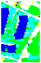
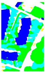
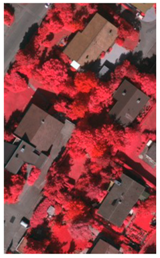
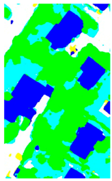
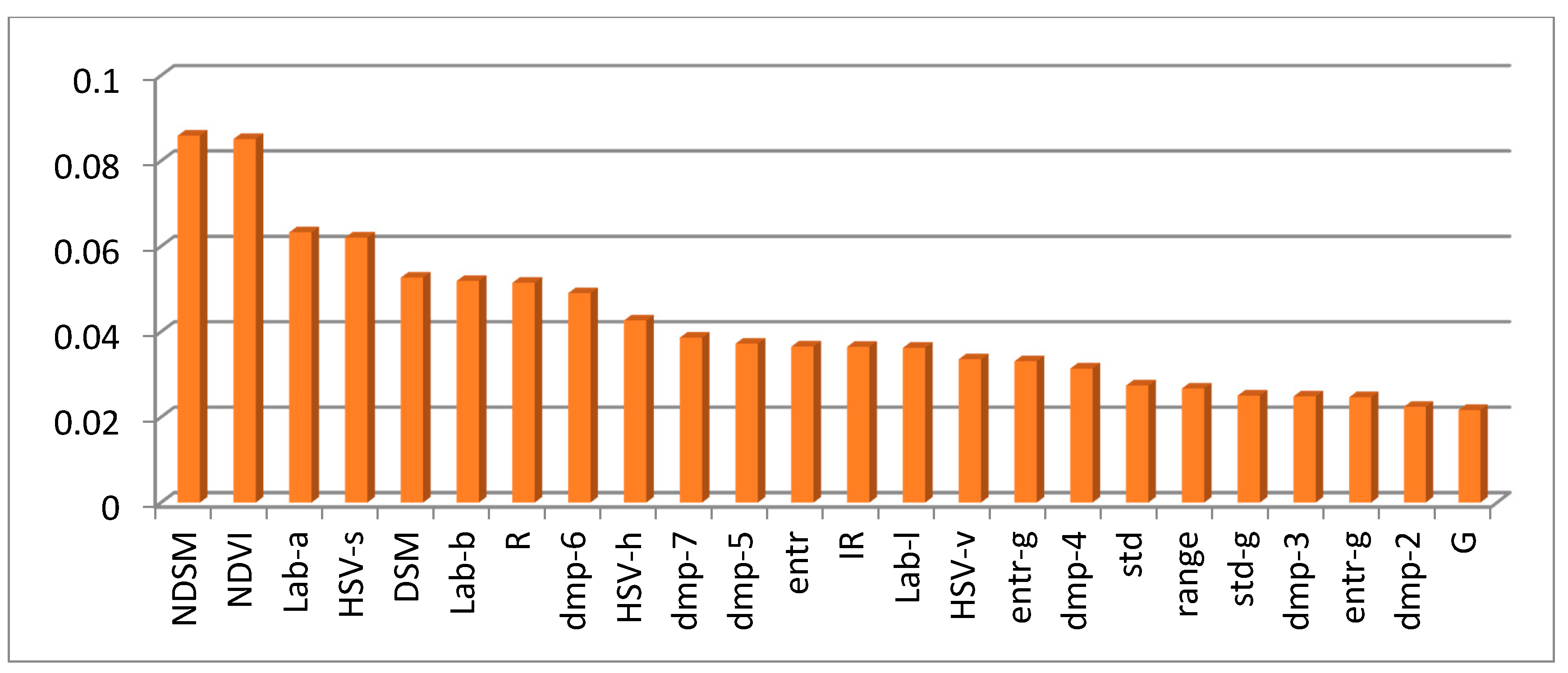
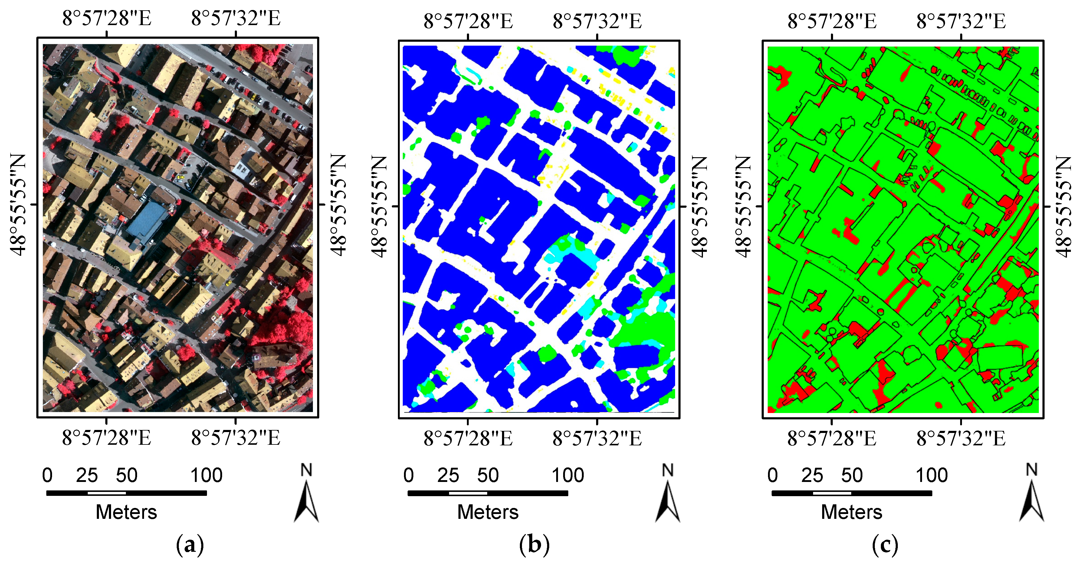
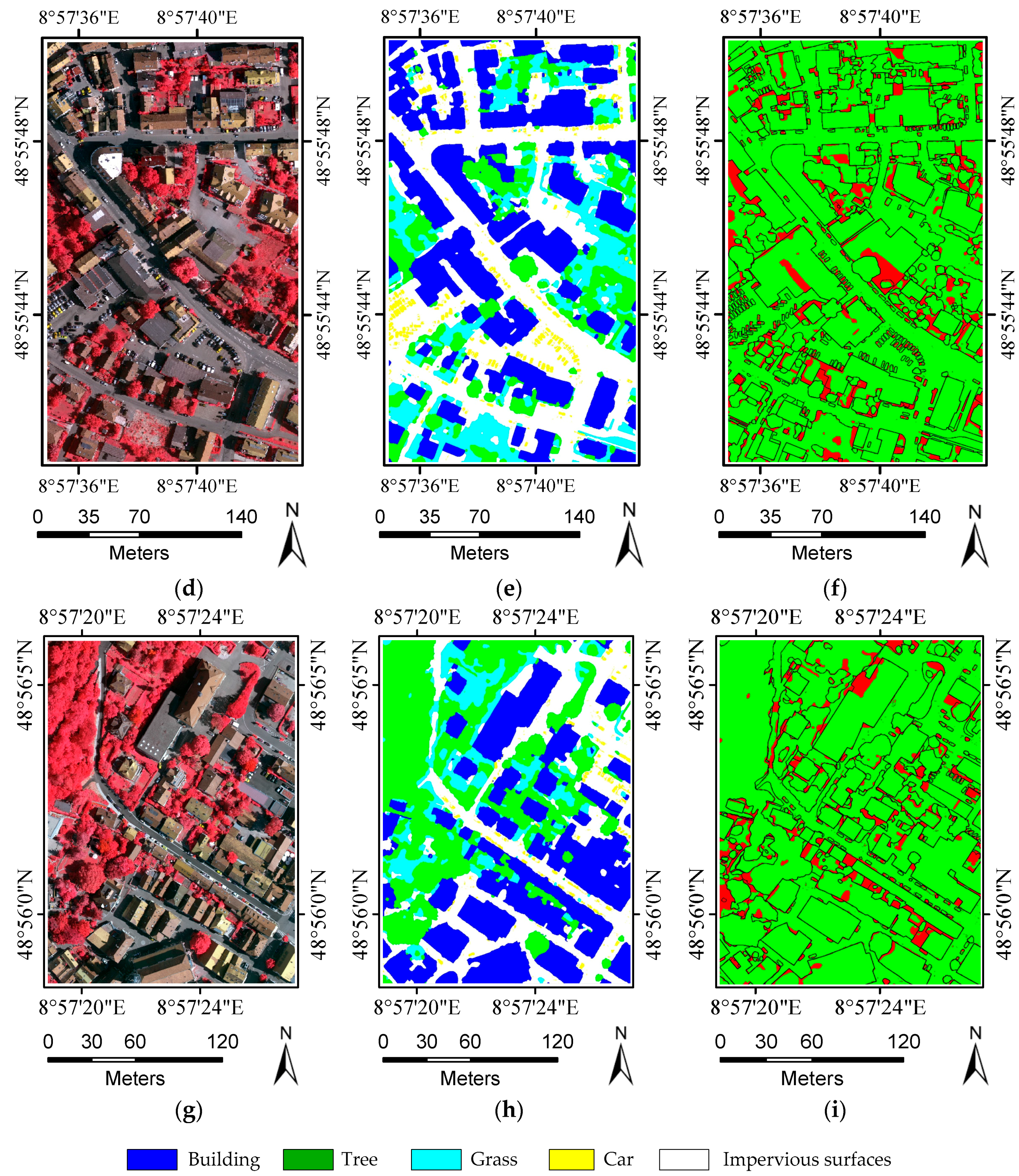
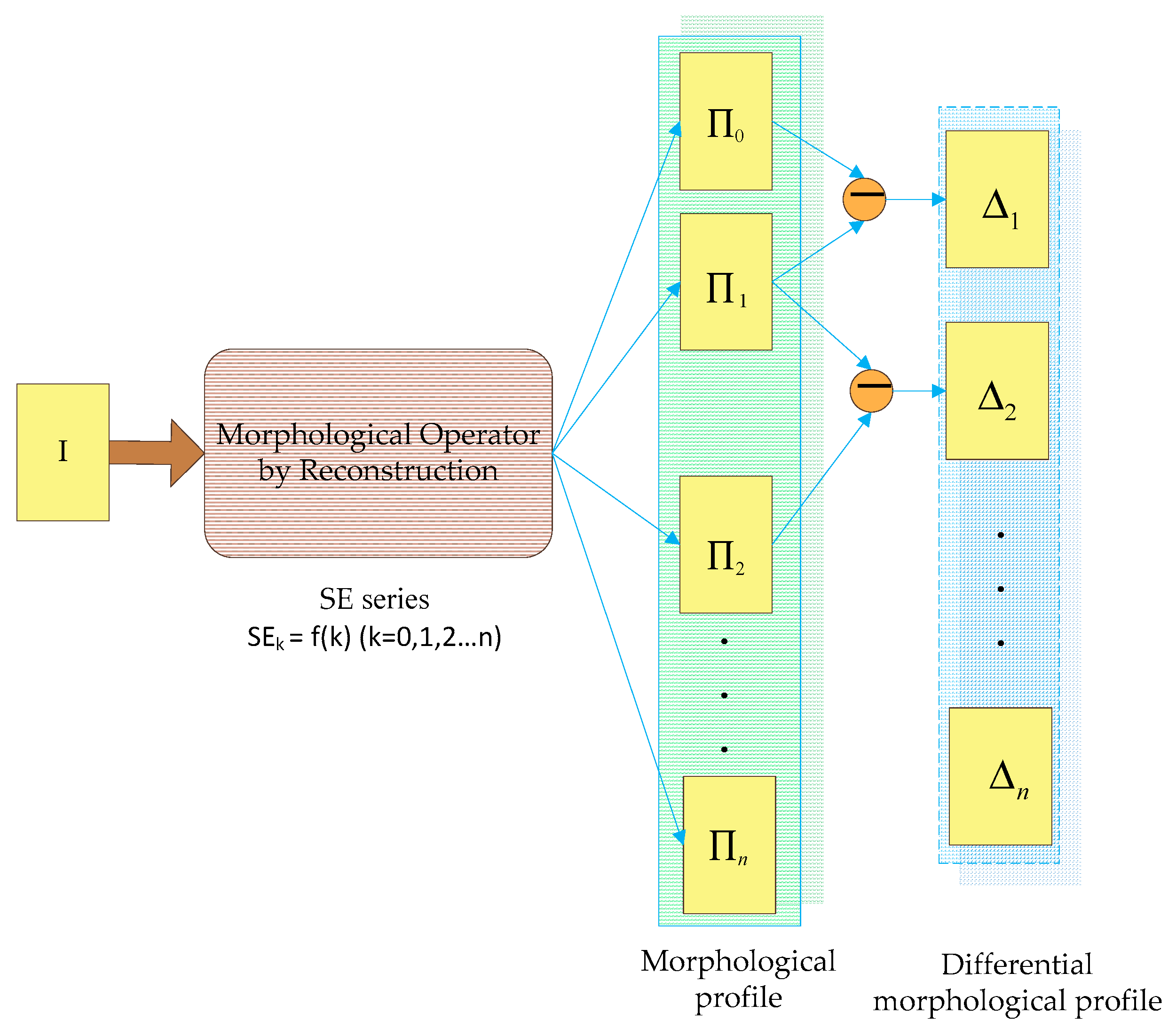
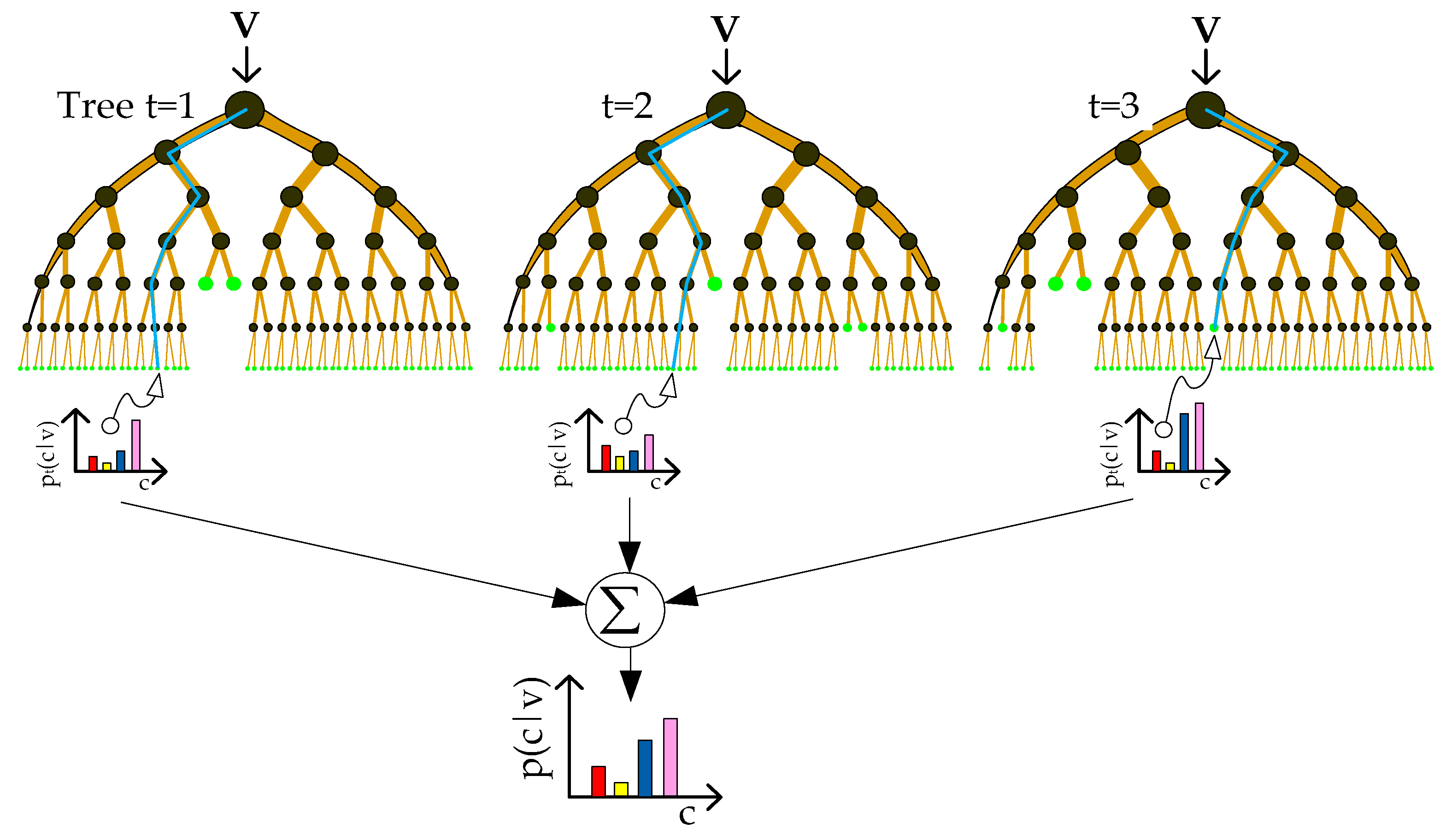
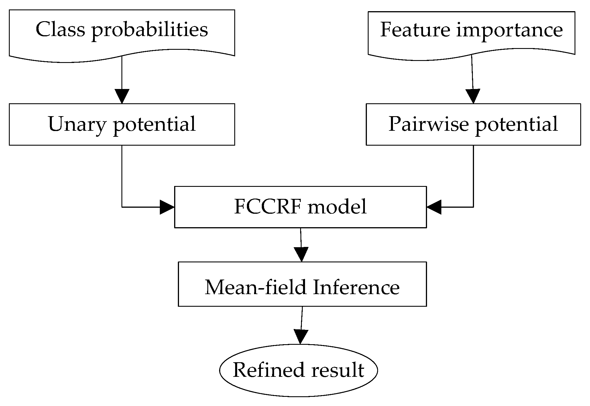
The current study combines methods from RF and probabilistic graphical models to classify high-resolution remote sensing data. Using high-resolution multispectral images and 3D geometry data, the method proceeds in three main stages: feature extraction, classification and refinement. A total of 13 features (color, vegetation index and texture) from the multispectral image and 11 features (height, elevation texture and DMP) from the 3D geometry data are first extracted to form the feature space. Then, the random forest is selected as the basic classifier for semantic classification. Inspired by the big training data and ensemble learning strategy adopted in the machine learning and remote sensing communities, a tile-based scheme is used to train multiple RFs separately. The multiple RFs are then combined to jointly predict the category probabilities of each sample. Finally, the probabilities and the feature importance indicators are used to construct an FCCRF graph model, and a mean-field-based statistical inference is carried out to refine the above classification results.

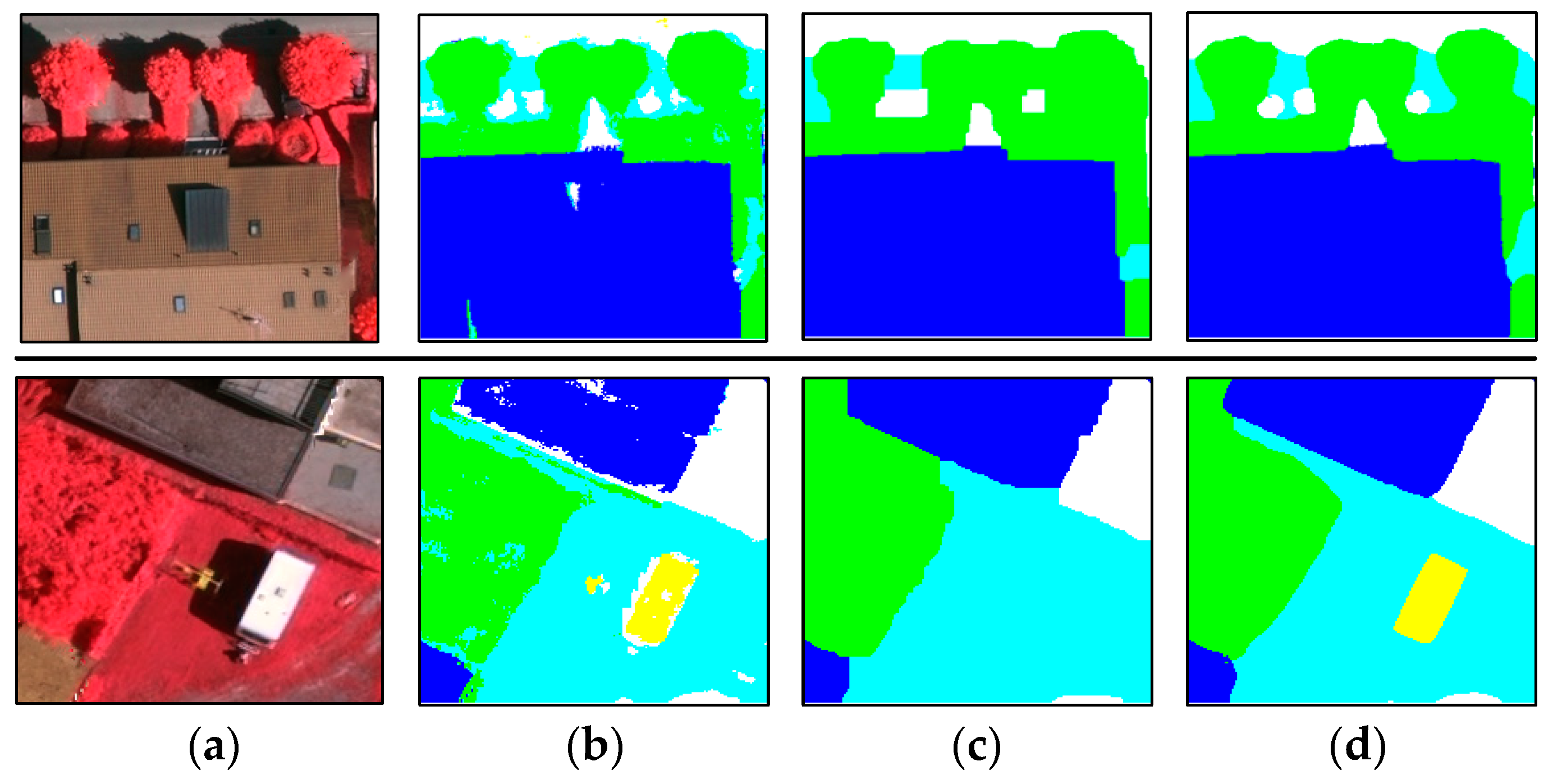
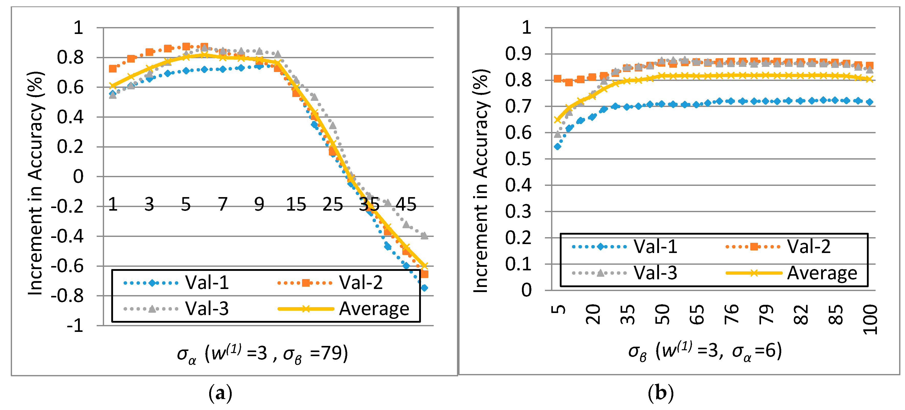
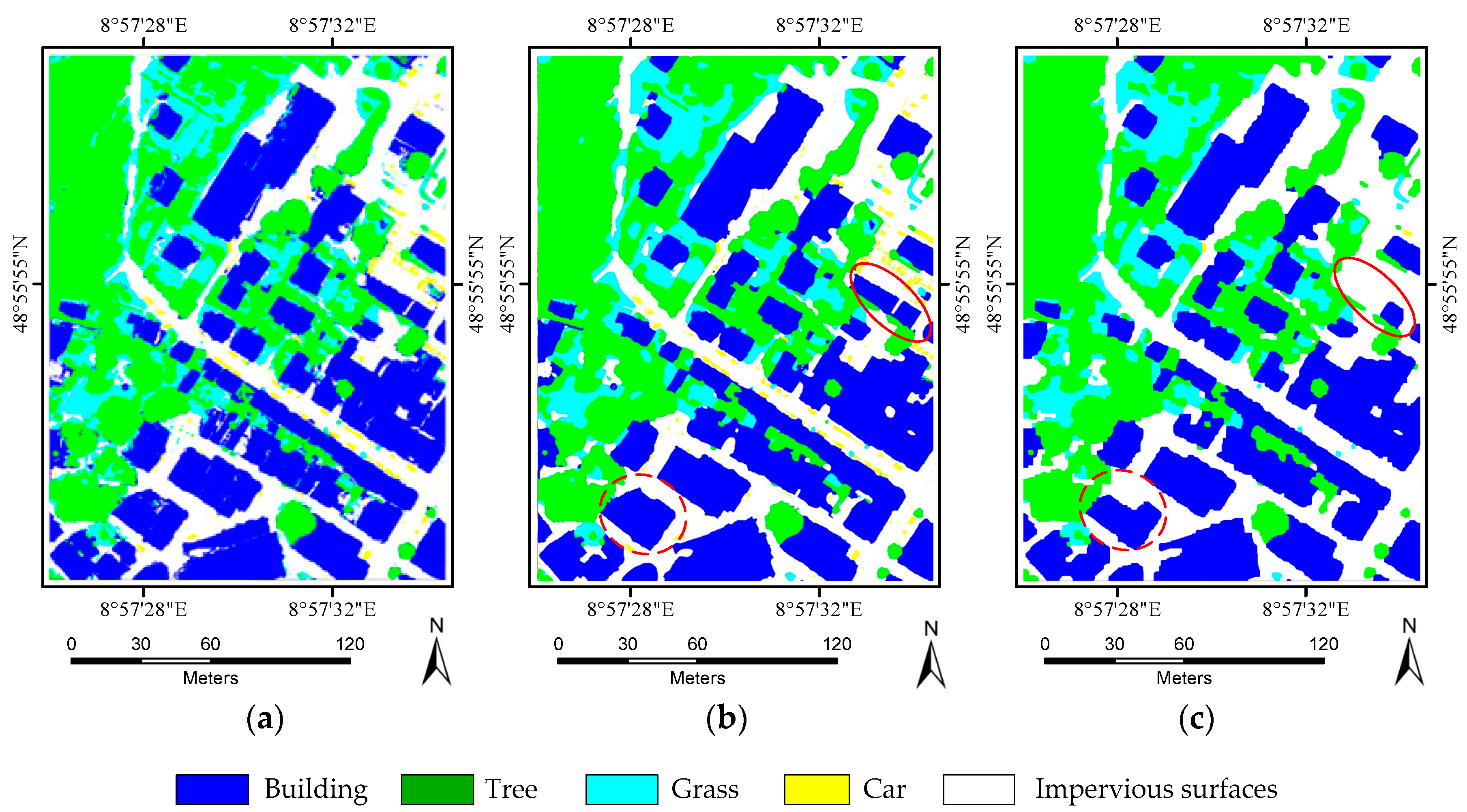
Experiments on the ISPRS Semantic Labeling Contest data show that features from both the multispectral image and the 3D geometry data are important and indispensable for the accurate semantic classification. Moreover, multispectral image-derived features play a greater role than the 3D geometry features. When comparing the classification accuracy of the single RF classifier and the fused RF ensemble, we found that both the generalization capability and the discriminability were enhanced significantly. Consistent with the conclusions drawn by others, the smoothness effect of the CRF is also evident in the presented work. Moreover, by introducing the 3 most important features to the pairwise potential of CRF, the classification accuracy is improved by approximately 1% in the presented experiments.

Note that in addition to urban land cover mapping, the current study can also be extended and used for other activities, such as vegetation mapping, water body mapping, and change detection.

Among the non-CNN-based methods, we achieve the highest overall accuracy, 86.9%. When compared to the CNN-based approaches, the gap between the current method and the best CNN method in the contest is still notable. However, we found that the presented method indeed outperformed several CNN-based methods. Furthermore, CNN can be conveniently integrated into the present RFE framework, as a feature extraction submodule to further boost the classification performance of the presented method. Hopefully, the integrated method could outperform the current best CNN method, which will be one of our future directions.

References

1. Paisitkriangkrai, S.; Sherrah, J.; Janney, P.; Hengel, A.V.-D. Effective semantic pixel labelling with convolutional networks and conditional random fields. In Proceedings of the 2015 IEEE Conference on Computer Vision and Pattern Recognition Workshops (CVPRW), Boston, MA, USA, 7–12 June 2015; pp. 36–43. [Google Scholar]
2. Lu, Q.; Huang, X.; Zhang, L. A novel clustering-based feature representation for the classification of hyperspectral imagery. Remote Sens. 2014, 6, 5732–5753. [Google Scholar] [CrossRef]
3. Benediktsson, J.A.; Palmason, J.A.; Sveinsson, J.R. Classification of hyperspectral data from urban areas based on extended morphological profiles. IEEE Trans. Geosci. Remote Sens. 2005, 43, 480–491. [Google Scholar] [CrossRef]
4. Shen, S. Accurate multiple view 3D reconstruction using patch-based stereo for large-scale scenes. IEEE Trans. Image Process. 2013, 22, 1901–1914. [Google Scholar] [CrossRef] [PubMed]
5. Furukawa, Y.; Ponce, J. Accurate, dense, and robust multiview stereopsis. IEEE Trans. Pattern Anal. Mach. Intell. 2010, 32, 1362–1376. [Google Scholar] [CrossRef] [PubMed]
6. Vosselman, G. Point cloud segmentation for urban scene classification. In Proceedings of the ISPR International Archives of the Photogrammetry, Remote Sensing and Spatial Information Sciences, Antalya, Turkey, 11–17 November 2013; Volume 40-7-W2, pp. 257–262. [Google Scholar]
7. Zhang, J.; Lin, X.; Ning, X. Svm-based classification of segmented airborne lidar point clouds in urban areas. Remote Sens. 2013, 5, 3749–3775. [Google Scholar] [CrossRef]
8. Zhang, J.; Lin, X. Advances in fusion of optical imagery and lidar point cloud applied to photogrammetry and remote sensing. Int. J. Image Data Fusion 2016, 8, 1–31. [Google Scholar] [CrossRef]
9. Rau, J.Y.; Jhan, J.P.; Hsu, Y.C. Analysis of oblique aerial images for land cover and point cloud classification in an urban environment. IEEE Trans. Geosci. Remote Sens. 2015, 53, 1304–1319. [Google Scholar] [CrossRef]
10. Gerke, M.; Xiao, J. Fusion of airborne laserscanning point clouds and images for supervised and unsupervised scene classification. ISPRS J. Photogramm. Remote Sens. 2014, 87, 78–92. [Google Scholar] [CrossRef]
11. Khodadadzadeh, M.; Li, J.; Prasad, S.; Plaza, A. Fusion of hyperspectral and lidar remote sensing data using multiple feature learning. IEEE J. Sel. Top. Appl. Earth Obs. Remote Sens. 2015, 8, 2971–2983. [Google Scholar] [CrossRef]
12. Zhang, Q.; Qin, R.; Huang, X.; Fang, Y.; Liu, L. Classification of ultra-high resolution orthophotos combined with dsm using a dual morphological top hat profile. Remote Sens. 2015, 7, 16422–16440. [Google Scholar] [CrossRef]
13. Chen, L.-C.; Papandreou, G.; Kokkinos, I.; Murphy, K.; Yuille, A.L. Semantic image segmentation with deep convolutional nets and fully connected CRFS. In Proceedings of the International Conference on Learning Representations (ICLR), San Diego, CA, USA, 7–9 May 2015. [Google Scholar]
14. Gerke, M. Use of the Stair Vision Library within the ISPRS 2D Semantic Labeling Benchmark (Vaihingen); Technical Report, ITC; University of Twente: Enschede, The Netherlands, 2015. [Google Scholar]
15. Marmanis, D.; Wegner, J.D.; Galliani, S.; Schindler, K.; Datcu, M.; Stilla, U. Semantic segmentation of aerial images with an ensemble of cnns. In Proceedings of the ISPRS Annals of the Photogrammetry, Remote Sensing and Spatial Information Sciences, Prag, Tschechien, 12–19 July 2016; Volume 3, pp. 473–480. [Google Scholar]
16. Niemeyer, J.; Rottensteiner, F.; Soergel, U. Classification of urban lidar data using conditional random field and random forests. In Proceedings of the 2013 Joint Urban Remote Sensing Event (JURSE), Sao Paulo, Brazil, 21–23 April 2013. [Google Scholar]
17. Speldekamp, T.; Fries, C.; Gevaert, C.; Gerke, M. Automatic Semantic Labelling of Urban Areas Using a Rule-Based Approach and Realized with Mevislab; Technical Report; University of Twente: Enschede, The Netherlands, 2015. [Google Scholar]
18. Wei, Y.; Yao, W.; Wu, J.; Schmitt, M.; Stilla, U. Adaboost-based feature relevance assessment in fusing lidar and image data for classification of trees and vehicles in urban scenes. In Proceedings of the ISPRS Annals of the Photogrammetry, Remote Sensing and Spatial Information Sciences, Melbourne, Australia, 25 August–1 September 2012. [Google Scholar]
19. Krizhevsky, A.; Sutskever, I.; Hinton, G.E. Imagenet classification with deep convolutional neural networks. In Proceedings of the Neural Information Processing Systems Conference, Lake Tahoe, NV, USA, 3–8 December 2012. [Google Scholar]
20. Sermanet, P.; Eigen, D.; Zhang, X.; Mathieu, M.; Fergus, R.; Lecun, Y. Overfeat: Integrated recognition, localization and detection using convolutional networks. arXiv, 2014; arXiv:1312.6229. [Google Scholar]
21. Simonyan, K.; Zisserman, A. Very deep convolutional networks for large-scale image recognition. In Proceedings of the International Conference on Learning Representations (ICLR), San Diego, CA, USA, 7–9 May 2015. [Google Scholar]
22. He, K.; Zhang, X.; Ren, S.; Sun, J. Deep residual learning for image recognition. In Proceedings of the IEEE Conference on Computer Vision and Pattern Recognition (CVPR), Las Vegas, NV, USA, 27–30 June 2016. [Google Scholar]
23. Sherrah, J. Fully convolutional networks for dense semantic labelling of high-resolution aerial imagery. arXiv, 2016; arXiv:1606.02585. [Google Scholar]
24. Lin, G.; Shen, C.; Reid, I.; Hengel, A.V.D. Efficient piecewise training of deep structured models for semantic segmentation. In Proceedings of the IEEE Conference on Computer Vision and Pattern Recognition (CVPR), Las Vegas, NV, USA, 27–30 June 2016; pp. 3194–3203. [Google Scholar]
25. Long, J.; Shelhamer, E.; Darrell, T. Fully convolutional networks for semantic segmentation. In Proceedings of the IEEE Conference on Computer Vision and Pattern Recognition (CVPR), Boston, MA, USA, 7–12 June 2015. [Google Scholar]
26. Papandreou, G.; Chen, L.C.; Murphy, K.P.; Yuille, A.L. Weakly-and semi-supervised learning of a deep convolutional network for semantic image segmentation. In Proceedings of the IEEE International Conference on Computer Vision (ICCV), Santiago, Chile, 13–16 December 2015; pp. 1742–1750. [Google Scholar]
27. Penatti, O.A.B.; Nogueira, K.; Santos, J.A.D.S. Do deep features generalize from everyday objects to remote sensing and aerial scenes domains? In Proceedings of the IEEE Conference on Computer Vision and Pattern Recognition Workshops (CVPRW), Boston, MA, USA, 7–12 June 2015. [Google Scholar]
28. Vaihingen 2D Semantic Labeling Contest. Available online: http://www2.Isprs.Org/vaihingen-2d-semantic-labeling-contest.html (accessed on 8 June 2017).
29. Ravinderreddy, R.; Kavya, B.; Ramadevi, Y. A survey on svm classifiers for intrusion detection. Int. J. Comput. Appl. 2014, 98, 34–44. [Google Scholar] [CrossRef]
30. Hsu, C.-W.; Lin, C.-J. A comparison of methods for multiclass support vector machines. IEEE Trans. Neural Netw. 2002, 13, 415–425. [Google Scholar] [PubMed]
31. Du, P.; Xia, J.; Zhang, W.; Tan, K.; Liu, Y.; Liu, S. Multiple classifier system for remote sensing image classification: A review. Sensors 2012, 12, 4764–4792. [Google Scholar] [CrossRef] [PubMed]
32. Lu, D.; Weng, Q. A survey of image classification methods and techniques for improving classification performance. Int. J. Remote Sens. 2007, 28, 823–870. [Google Scholar] [CrossRef]
33. Briem, G.J.; Benediktsson, J.A.; Sveinsson, J.R. Multiple classifiers applied to multisource remote sensing data. IEEE Trans. Geosci. Remote Sens. 2002, 40, 2291–2299. [Google Scholar] [CrossRef]
34. Waske, B.; Benediktsson, J.A. Fusion of support vector machines for classification of multisensor data. IEEE Trans. Geosci. Remote Sens. 2007, 45, 3858–3866. [Google Scholar] [CrossRef]
35. Ceamanos, X.; Waske, B.; Benediktsson, J.A.; Chanussot, J.; Fauvel, M.; Sveinsson, J.R. A classiler ensemble based on fusion of support vector machines for classifying hyperspectral data. Int. J. Image Data Fusion 2010, 1, 1–15. [Google Scholar] [CrossRef] [Green Version]
36. Vergara, L.; Soriano, A.; Safont, G.; Salazar, A. On the fusion of non-independent detectors. Digit. Signal Process. 2016, 50, 24–33. [Google Scholar] [CrossRef]
37. Stone, M.C. A Survey of Color for Computer Graphics. 2001. Available online: https://graphics.stanford.edu/courses/cs448b-02-spring/04cdrom.pdf (accessed on 10 August 2017).
38. Hunter, R.S. Photoelectric color-difference meter. J. Opt. Soc. Am. 1958, 48, 985–995. [Google Scholar] [CrossRef]
39. Awrangjeb, M.; Zhang, C.; Fraser, C.S. Building detection in complex scenes thorough effective separation of buildings from trees. Photogramm. Eng. Remote Sens. 2012, 78, 729–745. [Google Scholar] [CrossRef]
40. Dekker, R.J. Texture analysis and classification of ers sar images for map updating of urban areas in the netherlands. IEEE Trans. Geosci. Remote Sens. 2003, 41, 1950–1958. [Google Scholar] [CrossRef]
41. Putra, S.P.A.R.; Keat, S.C.; Abdullah, K.; San, L.H.; Nordin, M.N.M. Texture analysis of airsar images for land cover classification. In Proceedings of the 2011 IEEE International Conference on Space Science and Communication (IconSpace), Penang, Malaysia, 12–13 July 2011; pp. 243–248. [Google Scholar]
42. Texture Analysis. Available online: https://cn.Mathworks.Com/help/images/texture-analysis.html (accessed on 25 May 2017).
43. Khan, W.; Kumar, S.; Gupta, N.; Khan, N. A proposed method for image retrieval using histogram values and texture descriptor analysis. Int. J. Soft Comput. Eng. 2011, I, 33–36. [Google Scholar]
44. Ghamisi, P.; Benediktsson, J.A.; Sveinsson, J.R. Automatic spectral-spatial classification framework based on attribute profiles and supervised feature extraction. IEEE Trans. Geosci. Remote Sens. 2014, 52, 5771–5782. [Google Scholar] [CrossRef]
45. Pesaresi, M.; Benediktsson, J.A. A new approach for the morphological segmentation of high-resolution satellite imagery. IEEE Trans. Geosci. Remote Sens. 2001, 39, 309–320. [Google Scholar] [CrossRef]
46. Benediktsson, J.A.; Pesaresi, M.; Arnason, K. Classification and feature extraction for remote sensing images from urban areas based on morphological transformations. IEEE Trans. Geosci. Remote Sens. 2003, 41, 1940–1949. [Google Scholar] [CrossRef]
47. Ho, T.K. The random subspace method for constructing decision forests. IEEE Trans. Pattern Anal. Mach. Intell. 1998, 20, 832–844. [Google Scholar]
48. Ho, T.K. Random decision forests. In Proceedings of the International Conference on Document Analysis and Recognition, Montreal, QC, Canada, 14–16 August 1995; pp. 278–282. [Google Scholar]
49. Criminisi, A.; Shotton, J. Decision Forests for Computer Vision and Medical Image Analysis; Springer Science & Business Media: New York, NY, USA, 2013. [Google Scholar]
50. Breiman, L. Random forests. Mach. Learn. 2001, 45, 5–32. [Google Scholar] [CrossRef]
51. Verikas, A.; Gelzinis, A.; Bacauskiene, M. Mining data with random forests: A survey and results of new tests. Pattern Recognit. 2011, 44, 330–349. [Google Scholar] [CrossRef]
52. Strobl, C.; Boulesteix, A.-L.; Zeileis, A.; Hothorn, T. Bias in random forest variable importance measures: Illustrations, sources and a solution. BMC Bioinform. 2007, 8, 25. [Google Scholar] [CrossRef] [PubMed] [Green Version]
53. Reif, D.M.; Motsinger, A.A.; McKinney, B.A.; Crowe, J.E.; Moore, J.H. Feature selection using a random forests classifier for the integrated analysis of multiple data types. In Proceedings of the 2006 IEEE Symposium on Computational Intelligence and Bioinformatics and Computational Biology, Toronto, ON, Canada, 28–29 September 2006; pp. 1–8. [Google Scholar]
54. Ni, H.; Lin, X.; Zhang, J. Classification of als point cloud with improved point cloud segmentation and random forests. Remote Sens. 2017, 9, 288. [Google Scholar] [CrossRef]
55. Rodriguez-Galiano, V.F.; Ghimire, B.; Rogan, J.; Chica-Olmo, M.; Rigol-Sanchez, J.P. An assessment of the effectiveness of a random forest classifier for land-cover classification. ISPRS J. Photogramm. Remote Sens. 2012, 67, 93–104. [Google Scholar] [CrossRef]
56. Rother, C.; Kolmogorov, V.; Blake, A. Grabcut: Interactive foreground extraction using iterated graph cuts. In Proceedings of the ACM SIGGRAPH, Los Angeles, CA, USA, 8–12 August 2004. [Google Scholar]
57. Krahenbuhl, P.; Koltun, V. Efficient inference in fully connected CRFS with gaussian edge potentials. In Proceedings of the Conference on Neural Information Processing Systems (NIPS), Granada, Spain, 12–17 December 2011. [Google Scholar]
58. Boykov, Y.; Veksler, O.; Zabih, R. Fast approximate energy minimization via graph cuts. IEEE Trans. Pattern Anal. Mach. Intell. 2001, 23, 1222–1239. [Google Scholar] [CrossRef]
59. Conditional Random Field. Available online: http://www.Cs.Auckland.Ac.Nz/courses/compsci708s1c/lectures/glect-html/topic4c708fsc.htm (accessed on 28 May 2017).
60. Opper, M.; Saad, D. Advanced Mean Field Methods: Theory and Practice; MIT Press: Cambridge, MA, USA, 2001. [Google Scholar]
61. OpenCV. Available online: http://opencv.org/ (accessed on 11 June 2017).
62. Parameter Learning and Convergent Inference for Dense Random Fields. Available online: http://graphics.Stanford.Edu/projects/drf/ (accessed on 5 July 2017).
63. Kampffmeyer, M.; Salberg, A.-B.; Jenssen, R. Semantic segmentation of small objects and modeling of uncertainty in urban remote sensing images using deep convolutional neural networks. In Proceedings of the IEEE Conference on Computer Vision and Pattern Recognition Workshops (CVPRW), Las Vegas, NV, USA, 26 June–1 July 2016. [Google Scholar]
64. Pal, M. Random forest classifier for remote sensing classification. Int. J. Remote Sens. 2005, 26, 217–222. [Google Scholar] [CrossRef]
65. Vemulapalli, R.; Tuzel, O.; Liu, M.-Y.; Chellappa, R. Gaussian conditional random field network for semantic segmentation. In Proceedings of the IEEE Conference on Computer Vision and Pattern Recognition (CVPR), Las Vegas, NV, USA, 27–30 June 2016. [Google Scholar]
66. Mayer, H.; Hinz, S.; Bacher, U.; Baltsavias, E. A test of automatic road extraction approaches. Int. Arch. Photogramm. Remote Sens. Spat. Inf. Syst. 2006, 36, 209–214. [Google Scholar]
67. Piramanayagam, S.; Schwartzkopf, W.; Koehler, F.W.; Saber, E. Classification of remote sensed images using random forests and deep learning framework. J. Appl. Remote Sens. 2016, 100040L. [Google Scholar] [CrossRef]
68. Audebert, N.; Saux, B.L.; Lefèvre, S. On the usability of deep networks for object-based image analysis. In Proceedings of the International Conference on Geographic Object-Based Image Analysis (GEOBIA), Enschede, The Netherlands, 14–16 September 2016. [Google Scholar]
69. Marmanis, D.; Schindler, K.; Wegner, J.D.; Galliani, S.; Datcu, M.; Stilla, U. Classification with an edge: Improving semantic image segmentation with boundary detection. arXiv, 2016; arXiv:1612.01337. [Google Scholar]
70. Audebert, N.; Saux, B.L.; Lefevre, S. Semantic segmentation of earth observation data using multimodal and multi-scale deep networks. In Proceedings of the Asian Conference on Computer Vision (ACCV), Taipei, Taiwan, 21–23 November 2016. [Google Scholar]
71. Volpi, M.; Tuia, D. Dense semantic labeling of subdecimeter resolution images with convolutional neural networks. IEEE Trans. Geosci. Remote Sens. 2017, 55, 881–893. [Google Scholar] [CrossRef]
Figure 1. Pipeline of the proposed classification method.
Ijgi 06 00245 g001
Figure 2. Illustration of the basic principle of the DMP.
Ijgi 06 00245 g002
Figure 3. Classification process of RF (adapted from [49]).
Ijgi 06 00245 g003
Figure 4. Flowchart for RFE model training.
Ijgi 06 00245 g004
Figure 5. Tile-based samples selection and partition, where each type of sample consists of several tiles.
Ijgi 06 00245 g005
Figure 6. The results of two testing areas refined using short-range CRF and long-range FCCRF methods respectively. (a) the multispectral image; (b) the classification result from the RFE model; (c) the refined result from the short-range CRF model; (d) the refined result from the long-range FCCRF model.
Ijgi 06 00245 g006
Figure 7. Comparison of the short-range CRF and the fully connected CRF models. (a) In the short-range CRF, only the 4 nearest neighbors are connected to a certain node; (b) in the fully connected CRF, every two nodes are connected by an edge (from [59]).
Ijgi 06 00245 g007
Figure 8. Flowchart of the FCCRF-based refinement. The class probabilities and the feature importance indicators generated by the trained RFE model are used to construct the unary potential and the pairwise potential, respectively.
Ijgi 06 00245 g008
Figure 9. The true orthophoto of the test area, which is divided into 33 tiles.
Ijgi 06 00245 g009
Figure 10. Ground truth data used for the training and evaluation: (a) “full reference” ground truth; (b) “no boundary” ground truth, the black areas in this reference will be ignored during evaluation.
Ijgi 06 00245 g010
Figure 11. Feature importance indicator for classification, in descending order.
Ijgi 06 00245 g011
Figure 12. The classification results before and after the CRF refinement. (a) Classification map generated by the RFE; (b) The refined classification map produced by our long-range FCCRF; (c) The refined classification map produced by the classical short-range CRF.
Ijgi 06 00245 g012
Figure 13. Influence of the hyper parameter values ( w ( 1 ) , σ α and σ β ) on the final classification accuracy. The experiment is implemented on the 3 tiles (named Val-1, Val-2 and Val-3) of the validation set. (a) Influence of σ α ; (b) influence of σ β .
Ijgi 06 00245 g013
Figure 14. Influence of the original FCCRF hyper parameters values ( w ( 1 ) , σ α and σ β ) on the final classification accuracy. The experiment is implemented on the 3 tiles (named Val-1, Val-2 and Val-3) of the validation set. (a) Influence of σ α ; (b) influence of σ β .
Ijgi 06 00245 g014
Figure 15. Classification results of 3 areas evaluated on the ISPRS unseen testing set. Right (a,d,g) The original TOP (for better comparison); middle (b,e,h) the classified results obtained by the proposed method; right (c,f,i) the red/green error map (red pixels indicate wrongly classified pixels).
Ijgi 06 00245 g015aIjgi 06 00245 g015b