Article

A Two-Step Method for Missing Spatio-Temporal Data Reconstruction

1
State Key Lab of Resources and Environmental Information System, Institute of Geographic Sciences and Natural Resources Research, Chinese Academy of Sciences, Beijing 100101, China
2
Fujian Collaborative Innovation Center for Big Data Applications in Governments, Fuzhou 350003, China
3
Jiangsu Center for Collaborative Innovation in Geographical Information Resource Development and Application, Nanjing 210023, China
*
Author to whom correspondence should be addressed.
ISPRS Int. J. Geo-Inf. 2017, 6(7), 187; https://doi.org/10.3390/ijgi6070187
Submission received: 5 April 2017 / Revised: 8 June 2017 / Accepted: 19 June 2017 / Published: 23 June 2017

Abstract

:
Missing data reconstruction is a critical step in the analysis and mining of spatio-temporal data; however, few studies comprehensively consider missing data patterns, sample selection and spatio-temporal relationships. As a result, traditional methods often fail to obtain satisfactory accuracy or address high levels of complexity. To combat these problems, this study developed an effective two-step method for spatio-temporal missing data reconstruction (ST-2SMR). This approach includes a coarse-grained interpolation method for considering missing patterns, which can successfully eliminate the influence of continuous missing data on the overall results. Based on the results of coarse-grained interpolation, a dynamic sliding window selection algorithm was implemented to determine the most relevant sample data for fine-grained interpolation, considering both spatial and temporal heterogeneity. Finally, spatio-temporal interpolation results were integrated by using a neural network model. We validated our approach using Beijing air quality data and found that the proposed method outperforms existing solutions in term of estimation accuracy and reconstruction rate.

1. Introduction

Following both the rapid development and popularization of geographic information and the enhancement of data collection, data with temporal and spatial attributes are quickly accumulated and form large numbers of spatio-temporal datasets [1]; however, missing data are extremely common; for example, missing data on air quality monitoring sensor readings, missing data on floating car track points or the absence of mobile phone signaling records. If these gaps in data cannot be accurately filled, subsequent analysis and modeling of the data can lead to inaccurate results and unreasonable inference [2]. Simply deleting records containing missing data would lead to significant loss of original information and would be a waste of data resources [3]; therefore, methods to accurately and efficiently interpolate missing data are urgently needed.
In past decades, a large number of interpolation methods has been proposed to solve the problem of spatio-temporal missing data [4,5,6,7,8,9,10]. These methods can be roughly divided into three categories: spatial interpolation, temporal interpolation and spatio-temporal interpolation.
Spatial interpolation methods mainly use spatial correlation among data to interpolate missing data. Traditional methods (e.g., inverse distance weighting (IDW)) simply assume that the data distribution obeys the first law of geography, namely the closer data are in spatial distribution, the greater the contribution they make to missing data interpolation. During interpolation, each site is assumed to be independent of the others, and weights are calculated by computing the distance between missing data and the surrounding site [11,12]. Most approaches use kriging, a linear regression method that utilizes minimum mean square error and does not treat each site independently. The method assumes consistent sample mean and variance to meet second order stationarity and assumes that the covariance between any two spatio-temporal points is only associated with the distance (i.e., the absolute position of time and space is irrelevant) [13,14]. However, due to the existence of spatial and temporal heterogeneity, the data distribution can show uneven characteristics and relationships according to different regions [15]; therefore, the accuracy of interpolation results obtained by existing methods remains unsatisfactory if data are not homogeneously distributed. To solve this problem [16] considered spatial autocorrelation and heterogeneity in a study area and proposed a point estimation model of biased hospital-based area disease estimation (P-BSHADE). The P-BSHADE method calculates the covariance and correlation coefficient of historical observational data and uses the expectation between surrounding stations and interpolation sites to get an optimal linear unbiased estimator. However, in cases of continuous missing data, the method leads to a singular value of the missing data matrix, which results in large interpolation error. At the same time, this method does not consider the heterogeneity of the time dimension [2].
Time series prediction methods typically use historical data for a given location to build a prediction framework for predicting the values of missing data points at the same site. The autoregressive integrated moving-average (ARIMA) model [17] and simple exponential smoothing (SES) [18] are two representative examples of this approach. However, this approach fails to address two major problems. First, many prediction models do not fully utilize the essential characteristics of spatio-temporal data, which can degrade performance; second, if a consecutive series of data is all lost, prediction methods often cannot achieve complete reconstruction [19].
Given that single dimension interpolation methods only consider spatial or temporal dimensions, achieving satisfactory interpolation results is challenging. In recent years, a number of studies have extended single dimension interpolation methods to consider both space and time; for example, spatio-temporal probabilistic principal component regression (ST-PCR), spatio-temporal IDW (ST-IDW), spatio-temporal kriging (ST-kriging) and the spatio-temporal heterogeneous covariance method (ST-HC) [2,3,7,9,10,20,21,22]. ST-PCR [9] is a statistical learning-based method, which takes advantage of the statistical feature of observed data. However, it often needs a strong hypothesis over the data. ST-IDW [23] defined a three-dimensional space-time distance, which then applied IDW to estimate missing values; however, due to the existing problems with the IDW method, application of ST-IDW remains limited and fails to achieve unbiased estimation. The ST-kriging method [14] estimates the interpolation function by adopting a spatio-temporal covariance function, but it does not take into account the effects of spatial and temporal heterogeneity on interpolation results. To address this issue, the ST-HC method, which is an extension of P-BSHADE, estimates missing data by considering temporal and spatial heterogeneity. Missing datasets are firstly partitioned into homogenous spatial regions, and then, the most correlated spatial sampling and time sampling series are selected for the partition of missing data. According to the P-BSHADE algorithm, both spatial and temporal contribution weights are calculated to obtain the best linear unbiased estimates in spatial and temporal dimensions. Finally, using the correlation coefficient to determine the spatial and temporal weights, estimated values in spatial and temporal dimensions are integrated to obtain overall estimated values of missing data [
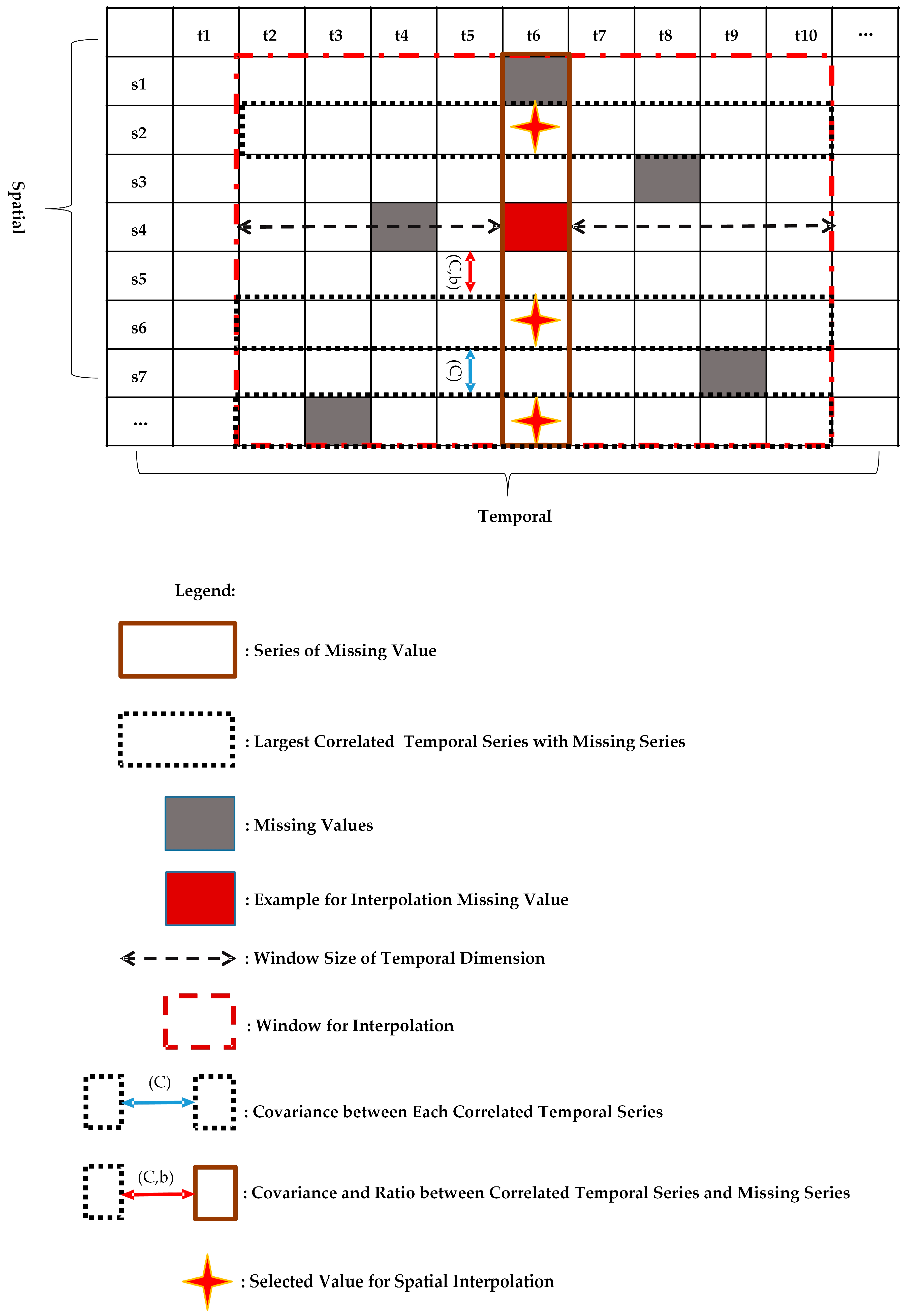
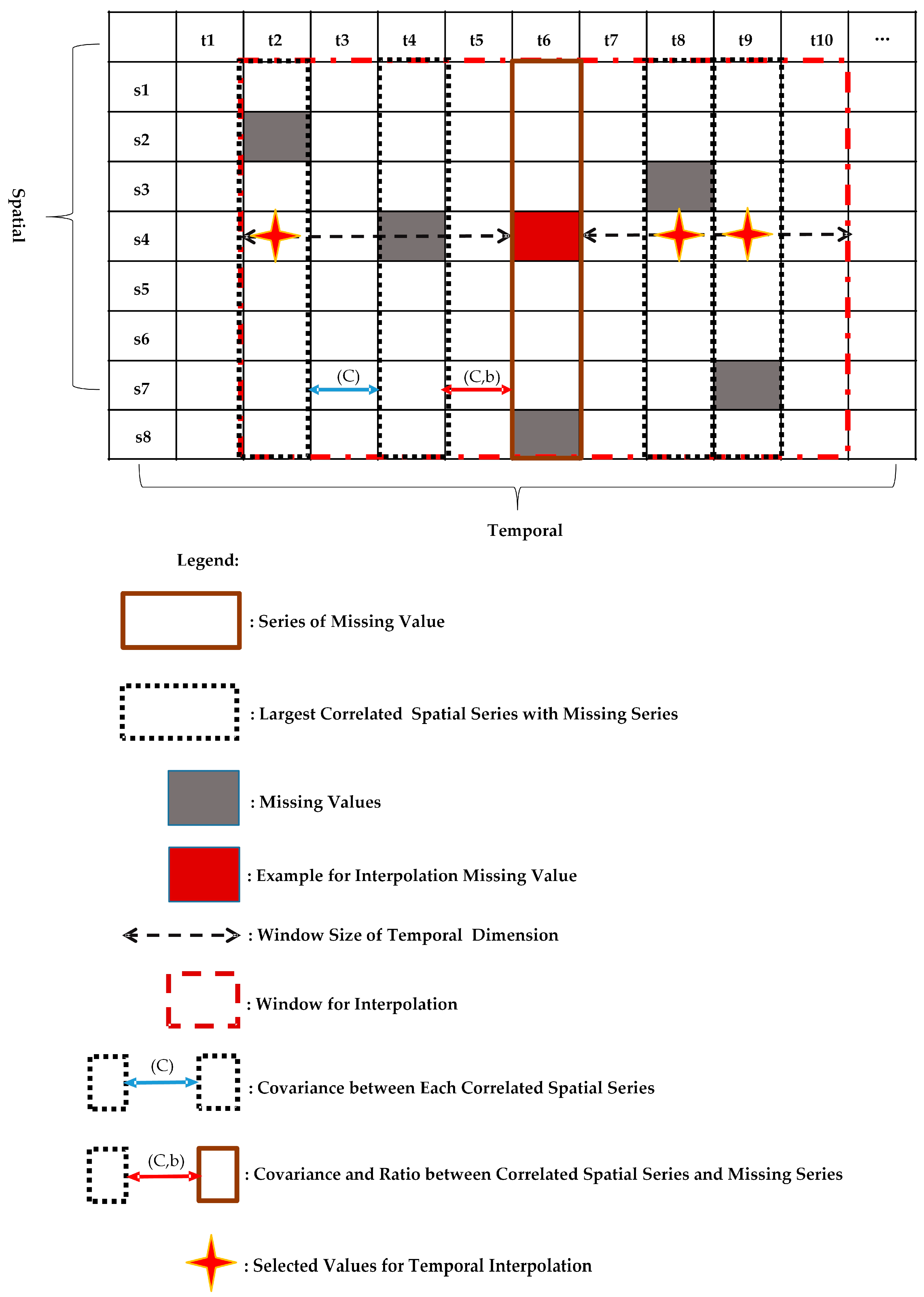
2]. However, this method requires the whole dataset to participate in computation, which leads to high computational complexity and a large volume of redundant data. For example, when the time span of the dataset is large, including the n dimensional space sequence, both n2 covariance and the correlation coefficient need to be calculated for each missing data point. In addition, when data are missing continuously, interpolation accuracy is low, and it may even be impossible to obtain a final interpolation result.
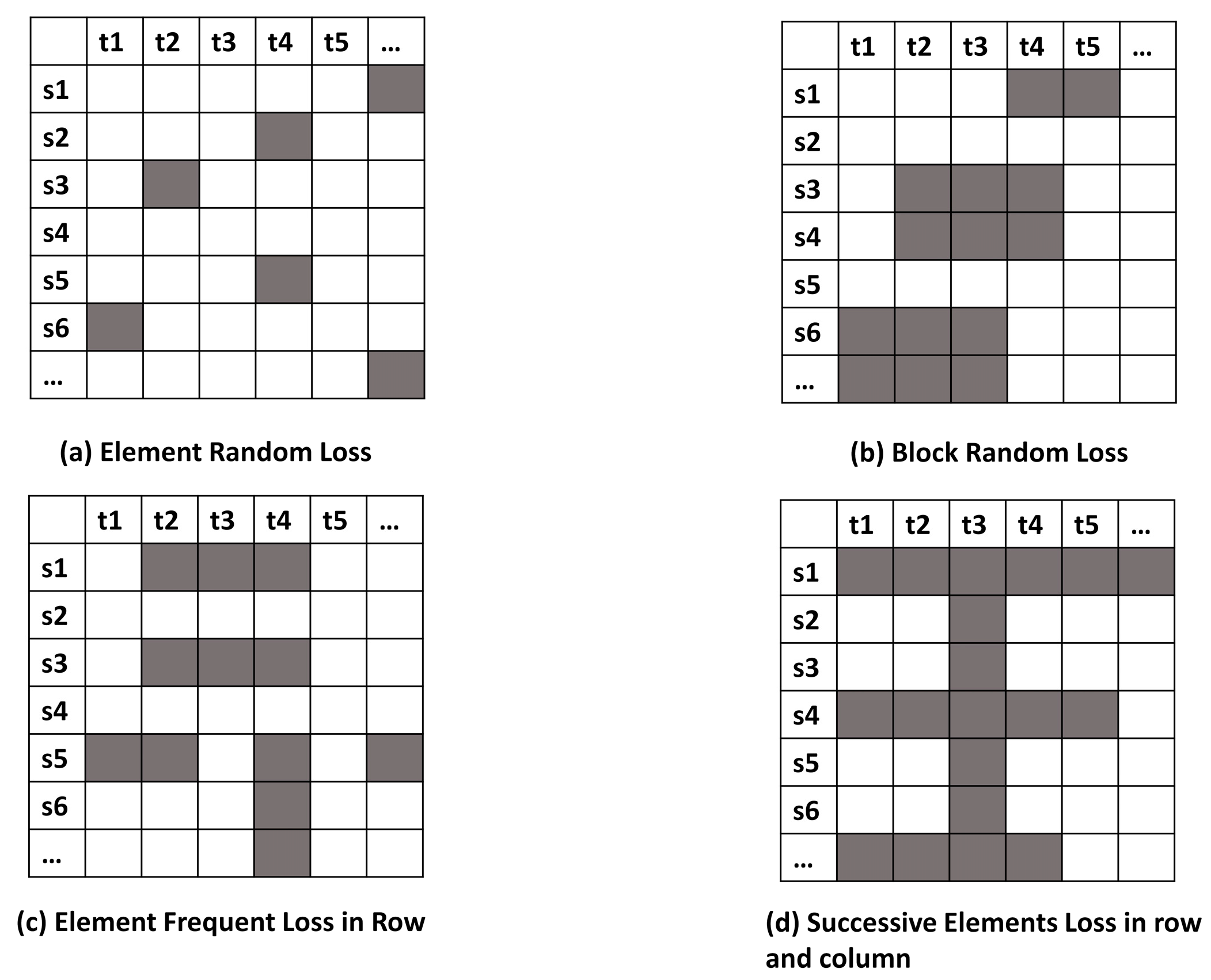
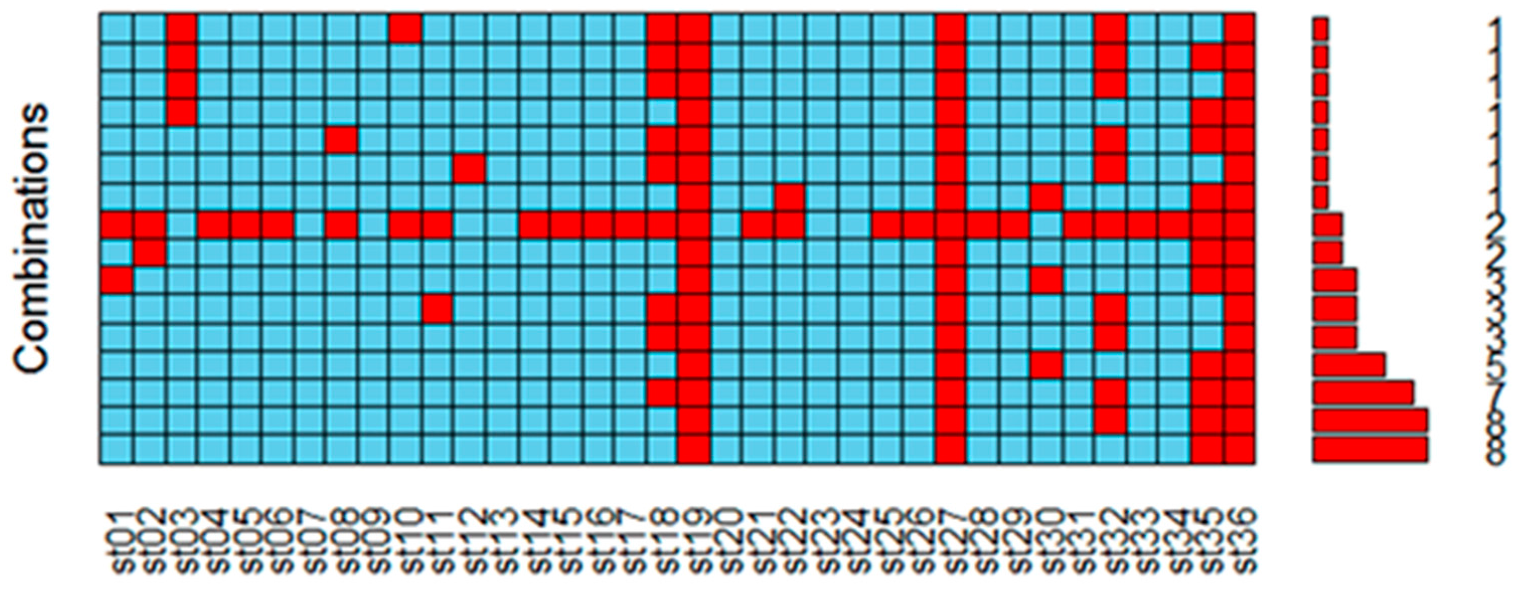
Missing data reconstruction methods are further challenged by the variation in patterns of missing data [24,25]; for example, missing data completely at random, non-random missing data [26], or whole blocks of missing data [27] (Figure 1). The work in [
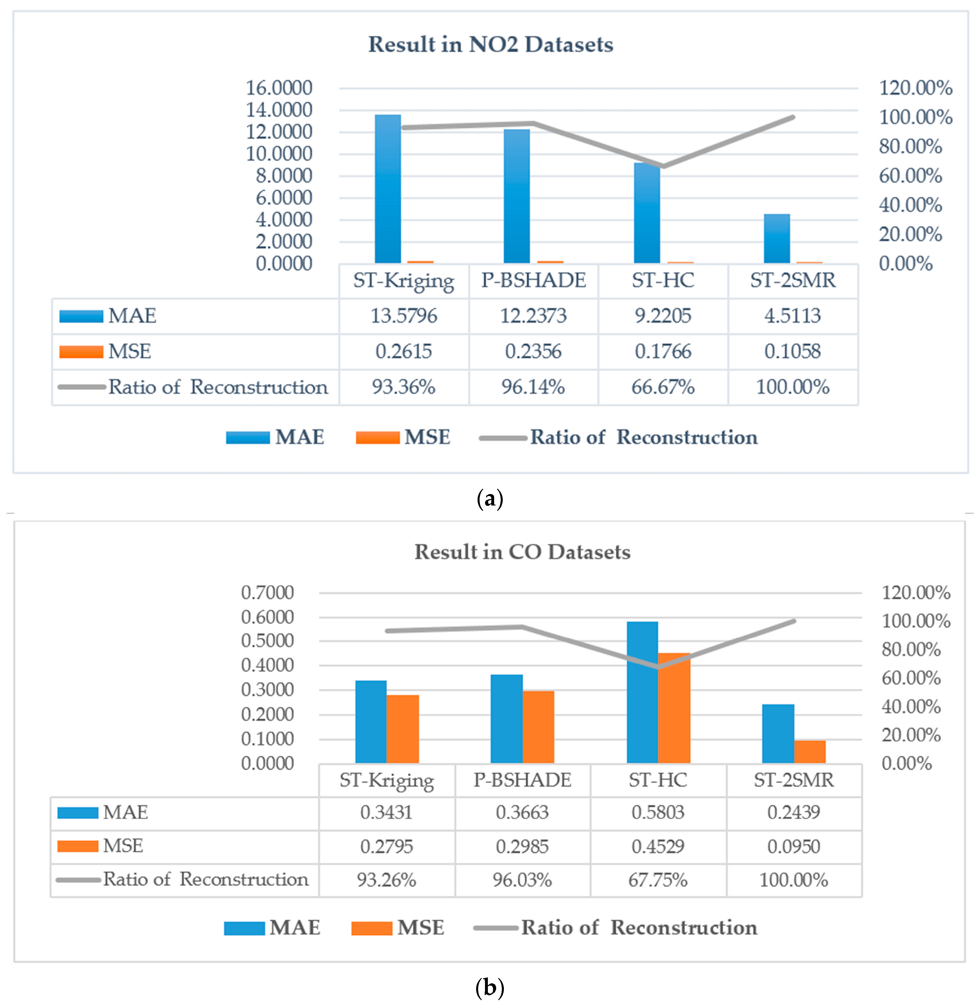
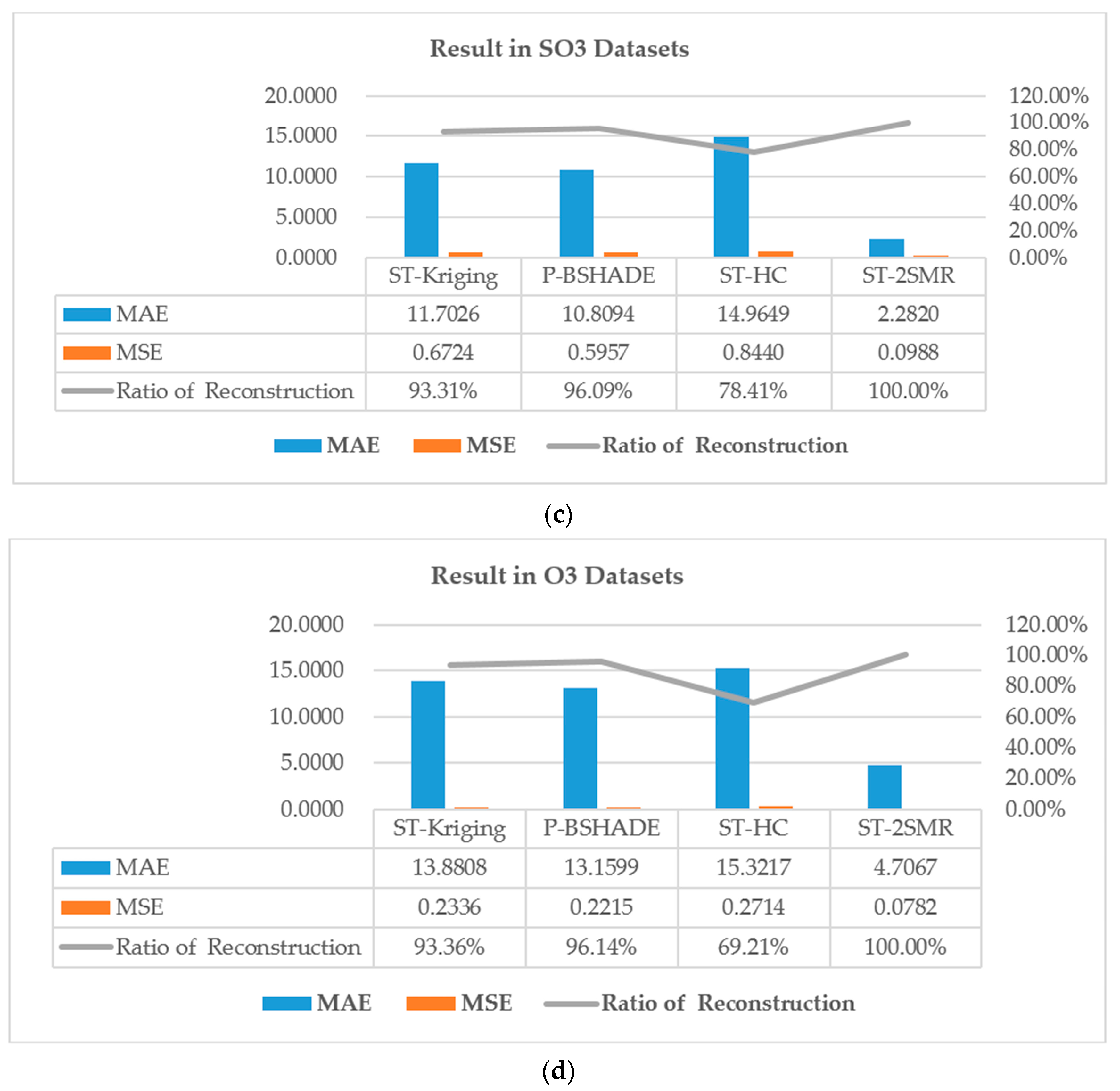
10] formulates the spatio-temporal sensory data as a high-dimensional tensor, using the tensor completion method to recover missing values. However, when a whole temporal or spatial dimension of the data is missing, this method may fail. The same problem exists for other spatio-temporal interpolation methods (e.g., IDW, kriging, P-BSHADE, ST-IDW, ST-kriging, ST-HC). Furthermore, most existing methods assume a linear relationship between spatial and temporal data (e.g., ST-HC, ST-IDW, ST-kriging); however, the relationship between spatial and temporal data may be linear or nonlinear. To address these issues, in this study, we developed a new two-step method to reconstruct missing spatio-temporal data (ST-2SMR).

2. Materials and Methods

2.1. Problem Definitions

Definition 1.
Suppose that y ( S , T ) represents a spatio-temporal missing dataset, where S and T are the spatial and temporal dimension, respectively; S = { s 1 , s 2 , , s m } , T = { t 1 , t 2 , , t n } , m is the total number of spatial objects and n is the total number of timestamps. An entry V i j = y ( s i , t j ) refers to the value of the i -th spatial object at the j -th timestamp ( 1 i m , 1 j n ) . The definition of the size of the sliding window is w ( 1 w n ). If there exist { V i j | ( j w 1 2 ) j ( j + w 1 2 ) } , then s i is a complete temporal sequence. If there exist { V i j   |   ( j w 1 2 ) j ( j + w 1 2 ) } , then s i exists, missing at the j-th timestamp. Similarly, if there exist { V i j | 1 i m } , then t j is a complete spatial sequence. If there exist { V i j | 1 i m } , it means that t j exists, missing at the i -th spatial object.
Definition 2.
Suppose that z i ^ = y ^ ( s i , t i ) is the estimated value of z i = y ( s i , t i ) , then the problem can be defined as:
{ m i n M S E = E ( z i ^ z i ) s . t . E ( z i ^ ) = z i
where MSE is the minimum mean square error and E is the statistical expectation. Meet E ( z i ^ ) = z i to ensure that the process of interpolation results in an unbiased estimate.

2.2. Method Framework

The method developed in this study (ST-2SMR) takes into account the problems of existing missing data interpolation methods and was constructed using 5 main steps (Figure 2): the partition of dataset into training and testing parts, coarse-grained interpolation, fine-grained interpolation, integration of temporal and spatial interpolation results and model performance evaluation.
  • First, because the ST-2SMR method uses a neural network model to combine the interpolation results in spatial and temporal dimensions, the space-time missing dataset was divided, with 80% selected for parameter training and 20% used as a test dataset to evaluate model performance, to avoid overfitting and to improve generalization ability.
  • Second, to avoid the influence of continuous missing data on fine-grained interpolation, coarse-grained interpolation for missing datasets was applied.
  • Based on the results of coarse-grained interpolation, spatial and temporal heterogeneity was used to perform fine-grained interpolation. During this process, it was necessary to calculate the correlation coefficient and covariance between time and space sequences to fit the parameters. If whole time series or spatial sequences are involved in interpolation, redundant sample data increase computational complexity; therefore, to improve the accuracy and speed of interpolation, a suitable sliding window was introduced to ensure the strongest correlation between sample data and missing data. Next, a heterogeneous covariance function was constructed for the space-time dimension. The best unbiased estimate of missing data can then be obtained by maximizing the objective function.
  • After interpolation of temporal and spatial dimensions, estimated values without missing data were chosen as training samples for the neural network, which is used to mine nonlinear relationships in spatio-temporal data. Estimated values of missing data were then obtained by inputting the spatio-temporal interpolation results of missing data into the trained neural network model.
  • Finally, the performance of the model was evaluated using the test dataset.

3. Detailed Design of ST-2SMR

3.1. Coarse-Grained Interpolation

Using existing spatial and temporal interpolation methods, it is difficult to obtain accurate interpolation estimates where there is a lack of sample points around missing points (Figure 1b,c). In some cases, it may even be impossible to obtain interpolation estimates (Figure 1d). We overcame this issue by introducing coarse-grained interpolation before fine-grained interpolation in order to eliminate the influence of continuous missing data. Using this approach, the ST-2SMR method is able to locate missing patterns in any combination, which ensures that the method is suitable for any serious loss situation.
In the spatial dimension, we used a classical multivariate statistical model (IDW) to interpolate missing data. IDW adopts the observed data of adjacent space points to estimate unknown data [11,28]. When the distance of the adjacent space points is closer to the point of interpolation, the spatial contribution value is larger. Interpolation estimates for missing data v _ s p a t i a l 0 ^ are calculated as follows:
v _ s p a t i a l 0 ^ = i = 1 m χ i v _ s p a t i a l i
χ i = d i α i = 1 m d i α
where d i denotes the distance between interpolation points and observation points and α is the decay weight rate, where a larger α denotes a faster decay by the distance.
In the time dimension, an exponential moving average model (SES) was used to estimate missing data [18]. SES assumes that there is strong temporal correlation between data, and the closer the sampling point is to the missing point, the bigger the weight that it is given. Traditional SES uses only the sampling data that are before the interpolation time point; however, when the time span is large, this can lead to too many irrelevant data involved in the calculation, which reduces interpolation accuracy. Here, we extended it to set a sliding window wc, which takes only before the wc time slice of the missing data and the last wc time slice of the missing data as the sampling point for the interpolation calculation. The model can be expressed as:
v _ t e m p o r a l 0 = ^ j = 1 w c v _ t e m p o r a l j β ( 1 β ) t h j 1 j = 1 w c β ( 1 β ) t h j 1
where v _ t e m p o r a l 0 ^ is the estimated value for missing data, t h j is a time interval between the sampling data and the missing data and β is a smoothing parameter with a range of (0, 1).
Assuming that V 4 , 6 are the data to be interpolated, we first selected all no missing data at t 6 , using IDW interpolation estimation (Figure 3). In the temporal dimension, we set the sliding window to be w c = 4 and selected { V 4 , 2 , V 4 , 3 , V 4 , 5 , V 4 , 7 , V 4 , 8 , V 4 , 10 } as the sampling data for interpolation. If both the IDW and SES methods can obtain an estimated value, the mean of the two is taken as the interpolation result of V 4 , 6 . If SES or IDW fail to get an interpolation result, the other estimated value is taken as the estimated value. If both SES and IDW fail to obtain an interpolation result, then V 4 , 6 is still missing, and the fine-grained interpolation algorithm is needed to estimate its value. The pseudocode of this process is shown in Algorithm 1.
Algorithm 1: Coarse-Grained interpolation.
Input: Original Missing Matrix V m × n
  Temporal Threshold w c
  Parameter of IDW α
  Parameter of SES β
Output: Coarse-Grained Imputing Matrix C _ M m × n
1 C _ M m × n I n i t i a l i z a t i o n ( V m × n )
2 For i = 1 to m
3For j = 1 to n
4  If V i j is missing value then
5    v c _ s p a t i a l 0
6    v c _ t e m p o r a l 0
7    v c _ s p a t i a l I D W ( V i j , α )
8      v c _ t e m p o r a l S E S ( V i j , β , w c )
9   If v c _ s p a t i a l , v c _ t e m p o r a l are not missing value then
10     C _ M i j ( v c _ s p a t i a l + v c _ t e m p o r a l ) / 2
11   Else if v c _ s p a t i a l is not missing value then
12     C _ M i j v c _ s p a t i a l
13   Else if v c _ t e m p o r a l is not missing value then
14     C _ M i j v c _ t e m p o r a l
15   Else
16     C _ M i j
17End for
18 End for

3.2. Fine-Grained Interpolation

3.2.1. Sliding Window

Before fine-grained interpolation, the ST-2SMR model needs to set up a dynamic sliding window to determine sample data. Owing to the strong temporal dependence of spatial and temporal data, selecting different numbers of data for interpolation estimation can lead to different results. If the window is set too small, sample data cannot fully reflect spatio-temporal relationships; if the window is too large (i.e., too many data are used), significant redundant data are introduced to the calculation, and the computational complexity increases.
Considering the fact that spatio-temporal data from a short period of time remain within the approximate correlation, take the average correlation of the missing data sequence and their adjacent spatial sequences to determine the optimal sample data using the expressions:
R b e g i n = 1 n w b e g i n j = n 1 w b e g i n C o r r ( t n , t j ) o b j e c t i v e : m i n w _ b e g i n s u b j e c t   t o :   R _ b e g i n = m a x ( R _ b e g i n )
R _ e n d = 1 w _ e n d n   i = n + 1 w _ e n d C o r r ( t n , t i ) o b j e c t i v e : m i n w _ e n d s u b j e c t   t o :   R _ e n d = m a x ( R _ e n d )
where n is the timestamp for missing data, j are the first j moments of missing data, i are the last i moments of missing data, C o r r ( t n , t j ) is the correlation coefficient between the spatial sequence of missing data and the first j spatial sequences, C o r r ( t n , t i ) is the correlation coefficient between the spatial sequence of missing data and the last i spatial sequences, w _ b e g i n is the beginning of the window and w _ e n d is the end of the window. w _ b e g i n and w _ e n d are determined heuristically and are initially set to n 1 and n + 1 . C o r r ( t n , t j ) and C o r r ( t n , t i ) are first calculated, then w _ b e g i n moves forward, and w _ e n d moves backwards until the mean correlation coefficient reaches the maximum. Assuming that V 4 , 6 is the missing datum to be interpolated, t 6 is the spatial sequence of missing data, and t 2 ~ t 10 is the sliding window (Figure 4). The pseudocode of this process is shown in Algorithm 2.
Algorithm 2: Selected optimal window (SOM).
Input: Missing Spatial Series t n
Output: Start of Window w _ b e g i n
   End of Window w _ e n d
1 R _ b e g i n 0
2 R _ e n d 0
3 For j = n 1 to 1
4 R _ l a s t R _ b e g i n
5 R _ b e g i n ( R _ b e g i n + C o r r ( t n , t j ) ) / ( n j )
6If R _ b e g i n < R _ l a s t
7  Return j
8End if
9 End for
10 For i = n + 1 to end of the timestamp
11 R _ l a s t R _ e n d
12 R _ e n d ( R _ e n d + C o r r ( t n , t i ) ) / ( i n )
13If R _ e n d < R _ l a s t
14  Return i
15End if
16 End for
17 w _ b e g i n j
18 w _ e n d i

3.2.2. Fine-Grained Spatial Dimension Interpolation

In the spatial dimension, we first selected a sliding window based on the optimal window selection algorithm (SOM), whose size is w s . Assuming that V 4 , 6 is the missing data to be interpolated, the start and end positions of the selected window are centered on the V 4 , 6 in the first 4 columns and the last 4 columns of Figure 5. In this window, we chose the m s time series with the largest correlation of missing data. In detail, we adopted a pair-wise approach for calculating the correlation between the time series of missing data and its spatial neighbor sampling data, and then, m s spatial sampling data were selected to calculate the estimated value using the expression:
y 0 ^ = i = 1 m s w i y i
where y i denotes the i -th spatial neighbor sampling data of missing data and w i denotes the corresponding contribution weight of y i . As shown in Figure 5, suppose m s = 3 , if { s 2 , s 6 , s 8 } is the most relevant time series with missing data, then we take { V 2 , 6 , V 6 , 6 , V 8 , 6 } as the sampled data for interpolation.
In order to ensure y 0 ^ is an unbiased estimator of missing data, the following conditions must be satisfied:
E ( y 0 ^ ) = E ( y 0 )
where E ( . ) represents the statistical expectation. Considering the heterogeneity of the spatial dimension, we introduced the parameter b i to calculate the ratio between the statistical expectation of y 0 ^ and y 0 to characterize spatial heterogeneity.
b i = E ( y i ) / E ( y 0 )
Combining Formulae (7)–(9), the constraint condition of w i is as follows:
i = 1 m s w i b i = 1
In order to obtain the parameter w i , the objective function was constructed to minimize the variance between the missing and true data.
m i n w [ σ 2 y 0 ^ = E ( y 0 ^ y 0 ) 2 ]
Among them, Formula (11) can be resolved as follows:
σ 2 y 0 ^ = C ( y 0 ^ , y 0 ^ ) + C ( y 0 , y 0 ) 2 C ( y 0 ^ , y 0 ) = σ 2 y 0 + i = 1 m s j = 1 m s w i w j C ( y i , y j ) 2 i = 1 m s w i C ( y i , y j )
where C represents the covariance between different spatial points. Considering Formula (10), Formulae (11) and (12) can be written as:
{ a r g w m i n σ 2 y 0 ^ = a r g m i n E ( y 0 ^ y 0 ) 2 s . t . i = 1 m s w i b i = 1
Then, the problem of solving the parameter w i was transformed into a standard Lagrange constrained optimization problem, and Formula (13) was re-written as:
σ 2 y 0 ^ = σ 2 y 0 + i = 1 m s j = 1 m s w i w j C ( y i , y j ) 2 i = 1 m s w i C ( y i , y 0 ) + 2 μ ( i = 1 m s w i b i 1 )
where μ is a Lagrange multiplier. The partial derivatives of σ 2 y 0 ^ produces the equations:
δ σ 2 y 0 ^ δ w i = 0 = > 2 i = 1 m s w i C ( y i , y j ) 2 C ( y i , y 0 ) + 2 μ b i = 0 = > j = 1 m s w j C ( y i , y j ) + μ b i = C ( y i , y 0 )
Formula (15) can be written in the matrix form:
[ C ( y 1 , y 1 ) C ( y 1 , y m s ) b 1 C ( y m s , y 1 ) C ( y m s , y m s ) b m s b 1 b m s 0 ] [ w 1 w m s μ ] = [ C ( y 1 , y 0 ) C ( y m s , y 0 ) 1 ]
In order to obtain the parameter w i in Formula (16), we first calculated the covariance matrix C _ S between the most relevant temporal series and the ratio of statistical expectation b i and covariance C i between the most relevant temporal series and the missing temporal series (Lines 6–9 of Algorithm 3). Then, we joined these values into a matrix like Formula (16) and solved this matrix to get parameter w i (Lines 10–12 of Algorithm 3). Finally, through Formula (7), we obtained estimated values of missing data. As shown in Figure 5, parameter w i of V 4 , 6 can be calculated by: (1) obtaining the covariance of { s 2 , s 6 , s 8 } and the covariance C ( s 2 , s 4 ) , C ( s 6 , s 4 ) and C ( s 8 , s 4 ) ; (2) calculating the ratio of statistical expectation b 1 = E ( s 2 ) / E ( s 4 ) , b 2 = E ( s 6 ) / E ( s 4 ) and b 3 = E ( s 8 ) / E ( s 4 ) ; (3) obtaining weights w 1 , w 2 and w 3 by solving the matrix; and finally, (4) interpolating V 4 , 6 from w 1 × V 2 , 6 + w 2 × V 6 , 6 + w 3 × V 8 , 6 .
Algorithm 3: Fine-Grained spatial interpolation.
Input: Coarse-Grained Matrix C _ M m × n
  Number of Spatial Neighbors m s
Output: Fine-Grained Spatial Matrix F _ S m × n
1 For i = 1 to m
2For j = 1 to n
3   w s S O M ( C _ M m × n , C _ M i j )
4   R s s C o r r c o e f ( M _ W m × w s , c o l u m n )
5   S _ C o r r e l a t e M a x   M s   C o r r e l a t e ( R s s , S _ M i s s i n g i , m s )
6   C _ S C o v ( S _ C o r r e l a t e )
7  For each S k S _ C o r r e l a t e
8    C k C o v ( S k , S _ M i s s i n g i )
9    b k M e a n ( S k ) / M e a n ( S _ M i s s i n g i )
10   C _ M a t r i x _ L e f t ( m s + 1 ) × ( m s + 1 ) C o m b i n e ( C _ S , b )
11   C _ M a t r i x _ R i g h t ( m s + 1 ) × 1 C o m b i n e ( C , 1 )
12   w C _ M a t r i x _ L e f t ( m s + 1 ) × ( m s + 1 ) C _ M a t r i x _ R i g h t ( m s + 1 ) × 1
13   F _ S i j D o t   P r o d u c t ( S _ C o r r e l a t e i , w )
14End for
15 End for

3.2.3. Fine-Grained Temporal Dimension Interpolation

In the temporal dimension, we used the SOM algorithm to select an optimal window as the data matrix for fine-grained temporal dimension interpolation. In this sliding window, the n t sample data with the largest correlation of missing data were chosen. The estimated value of missing data t 0 ^ was calculated as follows:
t 0 ^ = j = 1 n t φ j t j
where t j denotes the j -th temporal neighbor sampling data of missing data and φ j denotes the corresponding contribution weight of t j . Similar to Formulae (12)–(14), to ensure t 0 ^ is an unbiased estimator of missing data and to calculate the weight φ j , the following conditions must be satisfied:
σ 2 t 0 ^ = σ 2 t 0 j = 1 n t g = 1 n t φ j φ g C ( t j , t g ) 2 j = 1 n t φ j C ( t 0 ^ , t 0 ) + 2 v ( j = 1 n t φ j a j 1 )
where v is a Lagrange multiplier, t 0 is the true value of missing data and a j is the ratio of statistical expectation between the most relevant spatial series and the spatial series of missing data. The partial derivatives of σ 2 t 0 ^ can be written as:
δ σ 2 t 0 ^ δ φ i = 0 = > j = 1 n t φ j C ( t i , t j ) + v a j = C ( t i , t 0 )
Formula (19) can be written in the form of a matrix:
[ C ( t 1 , t 1 ) C ( t 1 , t n t ) a 1 C ( t n t , t 1 ) C ( t n t , t n t ) a n t a 1 a n t 0 ] [ φ 1 φ n t v ] = [ C ( t 1 , t 0 ) C ( t n t , t 0 ) 1 ]
As shown in Figure 6, in order to estimate the value of missing data V 4 , 6 , we first adopted the SOM algorithm to select t 2 t 10 as the sliding window. In this window, we choose the n t spatial series with the largest correlation of missing data. For example, when n t = 4 , the spatial series would be { t 2 , t 4 , t 8 , t 9 } , and we would take { V 4 , 2 , V 4 , 4 , V 4 , 8 , V 4 , 9 } as the sampled data for interpolation (Lines 3–5 of Algorithm 4). The covariance matrix C _ T was calculated from the most relevant spatial series and the ratio of statistical expectation a j and covariance C j by using the most relevant spatial series and the missing spatial series (Lines 6–9 of Algorithm 4). Then, we joined these values into matrix Formula (20) and solved this matrix to get parameter φ j (Lines 10–12 of Algorithm 4). Finally, through Formula (17), interpolation result V 4 , 6 was calculated as φ 1 × V 4 , 2 + φ 2 × V 4 , 4 + φ 3 × V 4 , 8 + φ 4 × V 4 , 9 .
Algorithm 4: Fine-Grained temporal interpolation.
Input: Coarse-Grained Matrix C _ M m × n
  Number of Temporal Neighbors n t
Output: Fine-Grained Temporal Matrix F _ T m × n
1 For i = 1 to m
2For j = 1 to n
3   w t S O M ( C _ M m × n , C _ M i j )
4   R t t C o r r c o e f ( M _ W m × w t , r o w )
5   T _ C o r r e l a t e M a x   N t   C o r r e l a t e ( R t t , T _ M i s s i n g j , n t )
6   C _ T C o v ( T _ C o r r e l a t e )
7  For each T k T _ C o r r e l a t e
8    C k C o v ( T k , T _ M i s s i n g j )
9    b k M e a n ( T k ) / M e a n ( T _ M i s s i n g j )
10   C _ M a t r i x _ L e f t ( n t + 1 ) × ( n t + 1 ) C o m b i n e ( C _ T , b )
11   C _ M a t r i x _ R i g h t ( n t + 1 ) × 1 C o m b i n e ( C , 1 )
12   φ C _ M a t r i x _ L e f t ( n t + 1 ) × ( n t + 1 ) C _ M a t r i x _ R i g h t ( n t + 1 ) × 1
13   F _ T i j D o t   P r o d u c t ( T _ C o r r e l a t e j , φ )
14End for
15 End for

3.3. Spatio-Temporal Integration

After obtaining interpolation results for the time and space dimensions, the BP (back propagation) neural network was trained to integrate spatial and temporal interpolation results to obtain final missing data estimation values [5]. The BP neural network can be regarded as a nonlinear function. When the number of input nodes is n, the output node is m, and the BP neural network expresses the mapping function from n independent variables to m dependent variables [29].
Appropriate samples are needed for training and testing neural networks. In this study, we first detect no missing data in the fine-grained temporal matrix F _ T m × n , fine-grained spatial matrix F _ S m × n and coarse-grained matrix C _ M m × n to construct the samples (Lines 1–7 of Algorithm 5). Then, the samples were divided into three parts: 80% as a training dataset, 10% as a test dataset and 10% as a cross-validation dataset to control early stopping (Lines 8–10 of Algorithm 5). Next, the error back-propagation algorithm was used to train the neural network model (Figure 7). Assuming that the input variables of the neural network model are X = { F _ S , F _ T } , the connection weights between the input layer and the hidden layer are γ i j and the hidden layer bias value is b i a s 1 , then the output of the hidden layer is:
H j = f ( i = 1 n γ i j x i b i a s l )   j = 1 , 2 , , l
where l is the number of hidden layer nodes and f is the activation function. Activation function f has many forms, from which we selected the sigmoid, which can be expressed as:
f ( x ) = 1 1 + e x
The interpolation estimate of missing data S T was calculated as follows:
S T = j = 1 l H j γ j 1 b i a s 2
where γ j 1 is the connection weight between the hidden layer and the output layer and b i a s 2 is the bias of the output layer. The weights and bias of Formula (23) can be calculated from:
γ i j = γ i j + η H j ( 1 H j )   x ( i ) γ j l e   i = 1 , 2 , , n ; j = 1 , 2 , , l γ j l = γ j l + η H j e   j = 1 , 2 , , l
b i a s 1 = b i a s 1 + η H j ( 1 H j ) w j l   j = 1 , 2 , , l b i a s 2 = b i a s 2 + e
where η is the learning rate and e is the prediction error of the neural network (i.e., the difference between the predicted and expected outputs). The training process of the neural network was completed when the algorithm reached the set of training objectives (i.e., the number of iterations and the minimum error).
After completing the neural network model, we were then able to predict the missing data. We first detected missing data in the coarse-grained matrix C _ M m × n . Then, the results of fine-grained spatial interpolation (FGSI) and fine-grained temporal interpolation (FGTI) algorithms were input to the neural network to calculate the estimated values (Lines 12–18 of Algorithm 5). Meanwhile, the results of FGSI and FGTI in the testing dataset were input to the neural network to evaluate the performance of the model (Lines 19–25 of Algorithm 5).
Algorithm 5: Combining spatial and temporal.
Input: Fine-Grained Spatial Matrix F _ S m × n
  Fine-Grained Temporal Matrix F _ T m × n
   Coarse-Grained Matrix C _ M m × n
   Number of Spatial Neighbors m s
   Number of Temporal neighbors n t
Output: Test Estimated Matrix S T m × n
   Missing Estimated Matrix M _ S T m × n
1  For i = 1 to m
2  For j = 1 to n
3   If F _ S i j F _ T i j     C _ M i j are not missing values then
4     S a m p l e S a m p l e ( F _ T i j , F _ S i j , C _ M i j )
5   End if
6  End for
7  End for
8   T r a i n i n g _ S p l D i v i d e ( S a m p l e ,     0.8 )
9   T e s t i n g _ S p l D i v i d e ( S a m p l e ,     0.1 )
10 C r o s s V a l i d a t i o n _ S p l D i v i d e ( S a m p l e ,     0.1 )
11 N e t T r a i n ( T r a i n i n g _ S p l ) N e u r a l   N e t w o r k   T r a i n i n g
12 For i = 1 to m
13For j = 1 to n
14  If C _ M i j is missing value then
15     M _ S T i j S i m ( N e t ,   F _ T i j , F _ S i j )
16   End if
17End for
18 End for
19 For i = 1 to m
20For j = 1 to n
21   If { F _ S i j , F _ T i j } T e s t i n g _ S p l then
22     S T i j S i m ( N e t ,   F _ T i j , F _ S i j )
23   End if
24End for
25 End for

4. Results

4.1. Datasets

We evaluated our model based on real air quality datasets from Beijing, which were collected between 5 January 2014 and 30 April 2015. Data included PM2.5, CO, SO3, O3, NO2 and other attributes, each of which was collected at 36 air quality monitoring stations at hourly intervals, as depicted in Figure 8. The dataset contained a total of 8759 records [30] (Table 1).
The different air quality variables have different degrees of missing data (Table 1). Among them, only PM2.5 contains a complete case. For the other attributes, we used combination analysis to explore the patterns of missing spatio-temporal missing data (Figure 9).
Using the PM2.5 dataset as an example, we set w t = 48 as the time sliding window, which took 48 h of data to explore the missing pattern. The missing numbers of st19, st27, st35 and st36 at the same time were eight (i.e., the missing pattern in Figure 1c). Data for st19, st27, st36 were completely missing (Figure 1d). Data for {st18, st19}, {st35, st36} showed random block loss (Figure 1b). Finally, a large number of patterns showed random missing data (Figure 1a). These patterns show that if the interpolation process was performed directly on the original dataset (i.e., without coarse-grained interpolation to eliminate the effect of successive missing data), it would be difficult to obtain accurate evaluation.

4.2. Evaluation Criteria

In order to evaluate the ST-2SMR method, we compared three existing methods (ST-kriging [31], P-BSHADE [16,32] and ST-HC [2,33]), each constrained in three different ways (i.e., increasing coarse-grained interpolation, increasing the sliding window or both; Table 2). We adopted mean absolute error (MAE), mean relative error (MRE) and the ratio of construction (RC) as the evaluation criteria to verify the performances of the proposed method.

4.3. Experimental Results

The proposed method was implemented in MATLAB 2016b. The PM2.5 dataset was selected to validate the proposed method. Through the comparative analysis of different experiments, the relevant parameters were set as follows: α = 4, β = 0.85, w c = 14, m s = 10, n t = 10, η = 0.01.

4.3.1. Overall Results

Among the first group of experiments (i.e., those using unaltered spatio-temporal interpolation methods), the ST-HC and ST-2SMR have the same reconstruction ratio, but different accuracy. The ST-2SMR method had the highest accuracy, reflecting in the effect of the nonlinear combination on the integration of spatial and temporal results (Table 3). The ST-HC and ST-2SMR have the same reconstruction ratio because they adopt the same spatio-temporal interpolation algorithm; however, the reconstruction rate was the lowest, which is owed to the introduction of heterogeneity in the time dimension. When we calculate the correlation coefficient and covariance between the spatial sequence of the missing data and the time slice, these sequences may seriously be missing. If the data sequence in the calculation is completely missing or using the pare-wise method makes the data sequence be completely missing, which may lead to the covariance matrix still having missing data, therefore we cannot get the final estimates, and this results in lower rate reconstruction.
In the second group of experiments (i.e., those with the original algorithms, but with the sliding window increased), interpolation precision was improved because the increased sliding window ensured that the sample data have the strongest correlation with missing data. In the third group of experiments (i.e., algorithms with coarse-grained interpolation added before the original interpolation method; here, we use IDW + SES as the coarse-grained interpolation method), the interpolation accuracy was also improved, and the complete reconstruction results were obtained because of the influence of continuous missing data has been eliminated. This result also validates the point of view in [34]: the accuracy and reliability of spatio-temporal interpolation methods depend on the pattern of missing data. However, interpolation accuracy improved the most when both constraints were applied at the same time, as demonstrated by the significant improvements in MAE and MSE (Table 3).

4.3.2. Effect of Coarse-Grained Interpolation

Through coarse-grained interpolation, continuous missing data were eliminated, significantly improving accuracy. Our experiments demonstrated that, regardless of the coarse-grained interpolation method chosen, interpolation accuracy improves when coarse-grained interpolation is first used (Table 4; here, we compare with the accuracy of those using unaltered spatio-temporal interpolation methods in Table 3). Among the methods tested, ST-2SMR showed the most significant improvement in accuracy, reflecting the nonlinear integration of spatial and temporal interpolation results, an approach that is particularly suitable for describing complex relationships between spatial and temporal data. However, overall, the accuracy of the IDW + SES method was found to be the best, so this method was chosen for coarse-grained interpolation in subsequent experiments.

4.3.3. Effect of the Coarse-Grained Missing Data Rate

According to Algorithm 1, the results of coarse-grained interpolation are mainly affected by the decay rate of weight α , smoothing parameter β and by time threshold wc. According to the experimental results of [27], performed using the same PM2.5 dataset, IDW and SES achieve a minimum MAE value when α = 4 and β = 0.85. For the time threshold, different values exert a significant influence on the coarse-grained interpolation results. In this study, we determined w c heuristically, with the value initially set to one (i.e., the center of missing data, taking the first hour and last hour as the sample data). With the increase in w c , the reconstruction rate of the missing data increased until complete reconstruction was achieved (Figure 10). We found that MAE was smallest when w c = 1 and stable when w c > 3. At w c > 3, the contribution weight of the sample data for missing data was nearly equal to zero, resulting in a small effect on the interpolation results. Furthermore, the termination condition of w c was set to ensure no continuous deletion of the whole space sequence and time series after coarse-grained interpolation, so as to obtain a complete interpolation result in the fine-grained interpolation. When w c < 14, the dataset from the coarse-grained interpolation still exhibited complete missing data in both the time and space sequences (Figure 11); therefore, fine-grained interpolation was required to achieve reconstruction. When w c = 14, coarse-grained interpolation eliminated the influence of successive missing data, so the reconstruction rate was 100%.

4.3.4. Effect Sample Point Number

During fine-grained interpolation, we were required to select m s spatial neighbors and n t temporal neighbors for missing data. The number of sample points impacted the assessment results. Too few sample data points fail to reflect the correlation of spatial and temporal data, while excessive sample data increase computational complexity and also reduce the accuracy of assessment because of redundant data. According to the experimental results of [16], when the number of sampling points is set to between five and 15, the interpolation results are perfect; therefore, we set three sets of adjacent point selection patterns (5, 10 and 15) in both the spatial and temporal dimensions (i.e., a total of nine sets of experiments) and performed experiments to determine the most suitable number of samples. When m s = 10 and n t = 10, the ST-2SMR method achieved its best performance (Table 5); however, the results show that the number of neighbor points had no effect on the reconstruction rate. This result reflects the elimination of continuous missing data during coarse-grained interpolation, which meant that all missing data had access to observed data for interpolation, allowing the whole dataset to obtain corresponding estimates.

4.3.5. Effect of Sliding Window

Our experimental results show that the SOM algorithm can dynamically select the size of each window through the interaction information for time and space (Figure 12). As a result, interpolation accuracy was greatly improved.

4.3.6. Performance of Two- and Three-Step Interpolation

In order to explore the convergence of the two-step interpolation, we further introduced a third-step interpolation (Table 6). The two-step interpolation used IDW + SES for coarse interpolation, while the three-step interpolation was based on the results of two-step interpolation using ST-kriging, P-BSHADE and ST-HC. The results demonstrate that three-step interpolation slightly improved accuracy, but the change was marginal. In addition, regardless of the method used for the third interpolation, the overall results tended to be stable; therefore, we concluded that the additional computational complexity of the three-step method was not justified by the minor improvement in performance.

4.3.7. Performance Comparison for Different Datasets

To verify the universality of the proposed method, the approach was tested using the NO2, CO, SO3 and O3 datasets (Figure 13). The results confirmed that the proposed method is superior to the other three methods in terms of accuracy. We found that only our new method can guarantee a complete reconstruction result and is able to maintain consistent stability across different datasets. For example, the P-BSHADE method performed better on the SO3 dataset, but worse for other datasets. The ST-HC method performed better on the NO2 dataset, but worse on the other datasets. This variable performance reflects the fact that different datasets have completely different missing data patterns, from which existing methods directly interpolate results (i.e., they do not eliminate the influence of missing patterns before interpolation).

4.3.8. Evaluation of Computational Efficiency

The computational efficiency is also an important factor worth evaluation for missing data reconstruction. We conducted a comparison of the computational efficiency on a 3.4-GHz Intel i7 CPU, with a 64-bit operating system, and 16.0 GM RAM. The CPU time costs of each interpolation method in the forecasting stages (i.e., we select 10% of samples as a test dataset) are shown in Figure 14. The computational efficiency of all of the four methods has no distinct difference. Obviously, ST-kriging is the fastest one among the interpolation methods because it does not take into account the effects of spatial and temporal heterogeneity on interpolation results. ST-HC and ST-2SMR consume only a little more time than ST-kriging and P-BSHADE because they are the extensions of P-BSHADE and consider the temporal and spatial heterogeneity. In addition, the linear combination of ST-HC to integrate spatio-temporal interpolation results almost spends the same time as nonlinear ways using a trained neural network, so the time complexity of ST-HC and ST-2SMR is nearly the same. However, the ST-2SMR method makes a significant trade-off between the efficiency and accuracy because the MSEs resulting from other methods are far larger than that of ST-2SMR (see Table 3). Therefore, when both efficiency and accuracy are considered, the proposed ST-2SMR outperforms the other methods.

5. Summary

Given the problem with existing missing data interpolation methods, this study developed a novel method called ST-2SMR. In the ST-2SMR method, missing data patterns in spatio-temporal datasets are first identified, and information on temporal and spatial dimensions is integrated to obtain a partial reconstruction. Using the output of this partial reconstruction, spatial and temporal heterogeneity is taken into account and a sliding window is set to both remove redundant sample data (i.e., to reduce computational complexity) and to ensure that the strongest correlation with missing data is selected (i.e., the most suitable data are chosen to improve the accuracy of the analysis). Finally, spatio-temporal interpolation results are integrated through a neural network model. We evaluated ST-2SMR using a real and open air quality dataset collected from Beijing. It is argued that the proposed method performs better than other existing methods. Providing the characteristics of the black box neural network models, the best way to integrate the results of spatio-temporal interpolation and to depict the nonlinear relationships between space and time requires further consideration.

Acknowledgments

This research is supported by the State Key Research Development Program of China (Grant No. 2016YFB0502104), the National Natural Science Foundation of China (41631177), and the Key Research Program of the Chinese Academy of Sciences (Grant No. ZDRW-ZS-2016-6-3). Their supports are gratefully acknowledged. And we also thank the anonymous referees for their helpful comments and suggestions.

Author Contributions

Shifen Cheng, Feng Lu conceived the idea for the research and wrote the paper; Shifen Cheng implemented the ST-2SMR model and carried out the experimental validation. Feng Lu interpreted the results and made the important comments and suggestions for this paper.

Conflicts of Interest

The authors declare no conflict of interest.

References

  1. Wang, J.; Yong, G.E.; Lianfa, L.I. Spatiotemporal data analysis in geography. Acta Geogr. Sin. 2014, 69, 1326–1345. [Google Scholar]
  2. Deng, M.; Fan, Z.; Liu, Q. A Hybrid Method for Interpolating Missing Data in Heterogeneous Spatio-Temporal Datasets. ISPRS Int. J. Geo-Inf. 2016, 5, 13. [Google Scholar] [CrossRef]
  3. Gao, Z.; Cheng, W.; Qiu, X. A Missing Sensor Data Estimation Algorithm Based on Temporal and Spatial Correlation. Int. J. Distrib. Sens. Netw. 2015, 2015, 1–10. [Google Scholar] [CrossRef]
  4. Galán, C.O.; Lasheras, F.S.; Juez, F.J.D.C.; Sánchez, A.B. Missing data imputation of questionnaires by means of genetic algorithms with different fitness functions. J. Comput. Appl. Math. 2017, 311, 704–717. [Google Scholar] [CrossRef]
  5. Durán-Rosal, A.M.; Hervás-Martínez, C.; Tallón-Ballesteros, A.J. Massive missing data reconstruction in ocean buoys with evolutionary product unit neural networks. Ocean Eng. 2016, 117, 292–301. [Google Scholar] [CrossRef]
  6. Tak, S.; Woo, S.; Yeo, H. Data-Driven Imputation Method for Traffic Data in Sectional Units of Road Links. IEEE Trans. Intell. Transp. Syst. 2016, 17, 1762–1771. [Google Scholar] [CrossRef]
  7. Tonini, F.; Dillon, W.W.; Money, E.S. Spatio-temporal reconstruction of missing forest microclimate measurements. Agric. For. Meteorol. 2016, 218–219, 1–10. [Google Scholar] [CrossRef]
  8. Londhe, S.; Dixit, P.; Shah, S. Infilling of missing daily rainfall records using artificial neural network. ISH J. Hydraul. Eng. 2015, 21, 255–264. [Google Scholar] [CrossRef]
  9. Tipton, J.; Hooten, M.; Goring, S. Reconstruction of spatio-temporal temperature from sparse historical records using robust probabilistic principal component regression. Adv. Stat. Clim. Meteorol. Oceanogr. 2017, 3, 1–16. [Google Scholar] [CrossRef]
  10. Ruan, W.; Xu, P.; Sheng, Q.Z. Recovering Missing Values from Corrupted Spatio-Temporal Sensory Data via Robust Low-Rank Tensor Completion; International Conference on Database Systems for Advanced Applications; Springer: Cham, Switzerland, 2017. [Google Scholar]
  11. Lu, G.Y.; Wong, D.W. An adaptive inverse-distance weighting spatial interpolation technique. Comput. Geosci. 2008, 34, 1044–1055. [Google Scholar] [CrossRef]
  12. Bartier, P.M.; Keller, C.P. Multivariate interpolation to incorporate thematic surface data using inverse distance weighting (IDW). Comput. Geosci. 1996, 22, 795–799. [Google Scholar] [CrossRef]
  13. Pesquer, L.; Cortés, A.; Pons, X. Parallel ordinary kriging interpolation incorporating automatic variogram fitting. Comput. Geosci. 2011, 37, 464–473. [Google Scholar] [CrossRef]
  14. Bhattacharjee, S.; Mitra, P.; Ghosh, S.K. Spatial Interpolation to Predict Missing Attributes in GIS Using Semantic Kriging. IEEE Trans. Geosci. Remote Sens. 2014, 52, 4771–4780. [Google Scholar] [CrossRef]
  15. Dutilleul, P. Spatio-Temporal Heterogeneity: Concepts and Analyses; Cambridge University Press: Cambridge, UK, 2011. [Google Scholar]
  16. Xu, C.; Wang, J.; Hu, M. Interpolation of Missing Temperature Data at Meteorological Stations Using P-BSHADE. J. Clim. 2013, 26, 7452–7463. [Google Scholar] [CrossRef]
  17. Yozgatligil, C.; Aslan, S.; Iyigun, C. Comparison of missing value imputation methods in time series: The case of Turkish meteorological data. Theor. Appl. Climatol. 2013, 112, 143–167. [Google Scholar] [CrossRef]
  18. Gardner, E.S., Jr. Exponential smoothing: The state of the art—Part II. Int. J. Forecast. 2006, 22, 637–666. [Google Scholar] [CrossRef]
  19. Li, Y.; Li, Z. Efficient missing data imputing for traffic flow by considering temporal and spatial dependence. Transp. Res. Part C Emerg. Technol. 2013, 34, 108–120. [Google Scholar] [CrossRef]
  20. Ran, B.; Tan, H.; Wu, Y. Tensor based missing traffic data completion with spatial-temporal correlation. Phys. A Stat. Mech. Appl. 2016, 446, 54–63. [Google Scholar] [CrossRef]
  21. Qi, H.; Liu, M.; Wang, D. Spatial-Temporal Congestion Identification Based on Time Series Similarity Considering Missing Data. PLoS ONE 2016, 11, e162043. [Google Scholar] [CrossRef] [PubMed]
  22. Holland, R.C.; Jones, G.; Benschop, J. Spatio-temporal modelling of disease incidence with missing covariate values. Epidemiol. Infect. 2015, 143, 1777–1788. [Google Scholar] [CrossRef] [PubMed]
  23. Reynolds, K.M.; Madden, L.V. Analysis of epidemics using spatio-temporal autocorrelation. Phytopathology 1988, 78, 240–246. [Google Scholar] [CrossRef]
  24. Li, D.; Deogun, J.; Spaulding, W. Towards Missing Data Imputation: A Study of Fuzzy K-means Clustering Method. Lect. Notes Comput. Sci. 2004, 3066, 573–579. [Google Scholar]
  25. Qu, L.; Li, L.; Zhang, Y. PPCA-based missing data imputation for traffic flow volume: A systematical approach. IEEE Trans. Intell. Transp. Syst. 2009, 10, 512–522. [Google Scholar]
  26. Kong, L.; Xia, M.; Liu, X.Y. Data Loss and Reconstruction in Sensor Networks. IEEE Infocom 2013, 25, 1654–1662. [Google Scholar]
  27. Yi, X.; Zheng, Y.; Zhang, J. ST-MVL: Filling Missing Values in Geo-Sensory Time Series Data. In Proceedings of the Twenty-Fifth International Joint Conference on Artificial Intelligence, IJCAI 2016, New York, NY, USA, 9–15 July 2016; pp. 2704–2710. [Google Scholar]
  28. Karydas, C.G.; Gitas, I.Z.; Koutsogiannaki, E. Evaluation of spatial interpolation techniques for mapping agricultural topsoil properties in Crete. EARSeL eProceedings 2009, 8, 26–39. [Google Scholar]
  29. Rumelhart, D.E.; Hinton, G.E.; Williams, R.J. Learning rep-resentation by back-propagating errors. Nature 1986, 323, 533–536. [Google Scholar] [CrossRef]
  30. Zheng, Y.; Yi, X.; Li, M. Forecasting fine-grained air quality based on big data. In Proceedings of the 21th ACM SIGKDD International Conference on Knowledge Discovery and Data Mining, Sydney, NSW, Australia, 10–13 August 2015. [Google Scholar]
  31. Cesare, L.D.; Myers, D.E.; Posa, D. Estimating and modeling space-time correlation structures. Stat. Probab. Lett. 2001, 51, 9–14. [Google Scholar] [CrossRef]
  32. Wang, J.F.; Li, X.H.; Christakos, G. Geographical Detectors-Based Health Risk Assessment and its Application in the Neural Tube Defects Study of the Heshun Region, China. Int. J. Geogr. Inf. Sci. 2010, 24, 107–127. [Google Scholar] [CrossRef]
  33. Fan, Z.; Gong, G.; Liu, B. A Space-time Interpolation Method of Missing Data Based on Spatio-temporal Heterogeneity. Acta Geod. Cartogr. Sin. 2016, 45, 458–465. [Google Scholar]
  34. Kondrashov, D.; Ghil, M. Spatio-temporal filling of missing points in geophysical data sets. Nonlinear Proc. Geophys. 2006, 13, 151–159. [Google Scholar] [CrossRef]
Figure 1. Patterns of missing spatio-temporal data. Black squares represent missing data.
Ijgi 06 00187 g001
Figure 2. Framework of model development.
Ijgi 06 00187 g002
Figure 3. Coarse-grained interpolation method.
Ijgi 06 00187 g003
Figure 4. Sliding window selection.
Ijgi 06 00187 g004
Figure 5. Fine-grained interpolation in the spatial dimension.
Ijgi 06 00187 g005
Figure 6. Fine-grained interpolation in the temporal dimension.
Ijgi 06 00187 g006
Figure 7. Neural network training.
Ijgi 06 00187 g007
Figure 8. Air quality monitoring stations.
Ijgi 06 00187 g008
Figure 9. Pattern of missing spatio-temporal PM2.5 data. Red squares represent missing data, and values on the right ordinate are the number of missing data combinations.
Ijgi 06 00187 g009
Figure 10. Impact of the temporal threshold on coarse-grained interpolation.
Ijgi 06 00187 g010
Figure 11. Impact of the temporal threshold on ST-2SMR.
Ijgi 06 00187 g011
Figure 12. Influence of the sliding window on the interpolation results. The static window refers to the selection of fixed size sliding window (i.e., the center of missing data, taking the first 24 h and last 24 h as the sample data for interpolation).
Ijgi 06 00187 g012
Figure 13. Performance of the ST-2SMR using different spatio-temporal datasets. (a) The result of the experiment in NO2 datasets; (b) The result of the experiment in CO datasets; (c) The result of the experiment in SO3 datasets; (d) The result of the experiment in O3 datasets .
Ijgi 06 00187 g013aIjgi 06 00187 g013b
Figure 14. Comparison of the computational time costs for different interpolation methods.
Ijgi 06 00187 g014
Table 1. Experimental dataset.
DataRatio of MissingComplete CaseNumber of Missing
PM2.513.25%29.11%41,771
CO15.10%0.00%47,604
SO315.24%0.00%48,041
O315.43%0.00%48,667
NO216.01%0.00%50,470
Table 2. Combination of different methods. P-BSHADE, point estimation model of biased hospital-based area disease estimation; ST, spatio-temporal; HC, heterogeneous covariance.
MethodCoarse-GrainedWindowCoarse-Grained + Window
ST-krigingST-kriging-CST-kriging-WST-kriging-C-W
P-BSHADEP-BSHADE-CP-BSHADE-WP-BSHADE-C-W
ST-HCST-HC-CST-HC-WST-HC-C-W
Table 3. Performance comparison of different methods. RC, ratio of construction; ST-2SMR, spatio-temporal missing data reconstruction.
ConditionMethodMAEMSERC
ST-Kriging18.37960.221196.20%
P-BSHADE18.20850.219096.20%
ST-HC26.42730.306665.94%
ST-2SMR15.52470.131965.94%
WindowST-Kriging-W14.32810.172499.60%
P-BSHADE-W14.61720.175899.29%
ST-HC-W11.22110.134993.69%
ST-2SMR9.59200.082293.69%
Coarse-GrainedST-Kriging-C13.17260.1585100%
P-BSHADE-C12.91780.1554100%
ST-HC-C8.76500.1054100%
ST-2SMR7.42920.0470100%
Coarse-Grained + WindowST-Kriging-C-W12.97170.1560100%
P-BSHADE-C-W12.66690.1524100%
ST-HC-C-W7.91960.0953100%
ST-2SMR7.22850.0623100%
Table 4. Performance of different coarse-grained interpolation methods 1. SES, simple exponential smoothing.
MethodIDW + SESST-KrigingP-BSHADE
MAEMREMAEMREMAEMRE
ST-kriging13.17260.158513.60270.163613.60100.1636
P-BSHADE12.91780.155413.58830.163513.60810.1637
ST-HC8.76500.10549.06370.10899.16010.1101
ST-2SMR7.42920.04707.48260.04757.60020.0484
1 The abscissa represents fine-grained interpolation; the ordinate represents coarse-grained interpolation.
Table 5. Influence sample point number on interpolation results.
Neighbor Station NumberMAEMRERC
SpatialTemporal
557.33000.0625100%
5107.32760.0635100%
5157.47360.0643100%
1057.27870.0630100%
10107.22850.0623100%
10157.27610.0630100%
1557.29520.0631100%
15107.28920.0631100%
15157.33320.0650100%
Table 6. Two- and three-step interpolation results.
MethodThree-StepTwo-Step
ST-KrigingP-BSHADEST-HCIDW + SES
MAEMREMAEMREMAEMREMAEMRE
ST-Kriging13.04980.157013.02350.156713.07410.157313.17260.1585
P-BSHADE12.78980.153912.79640.153912.83040.154312.91780.1554
ST-HC8.70750.10488.72060.10498.66180.10428.76500.1054
ST-2SMR7.41430.06517.42150.06527.40800.06417.42920.0470

