
A Lightweight CUDA-Based Parallel Map Reprojection Method for Raster Datasets of Continental to Global Extent

Abstract
:1. Introduction
2. Literature Review
3. Parallel Design and Implementation of Map Reprojections with CUDA
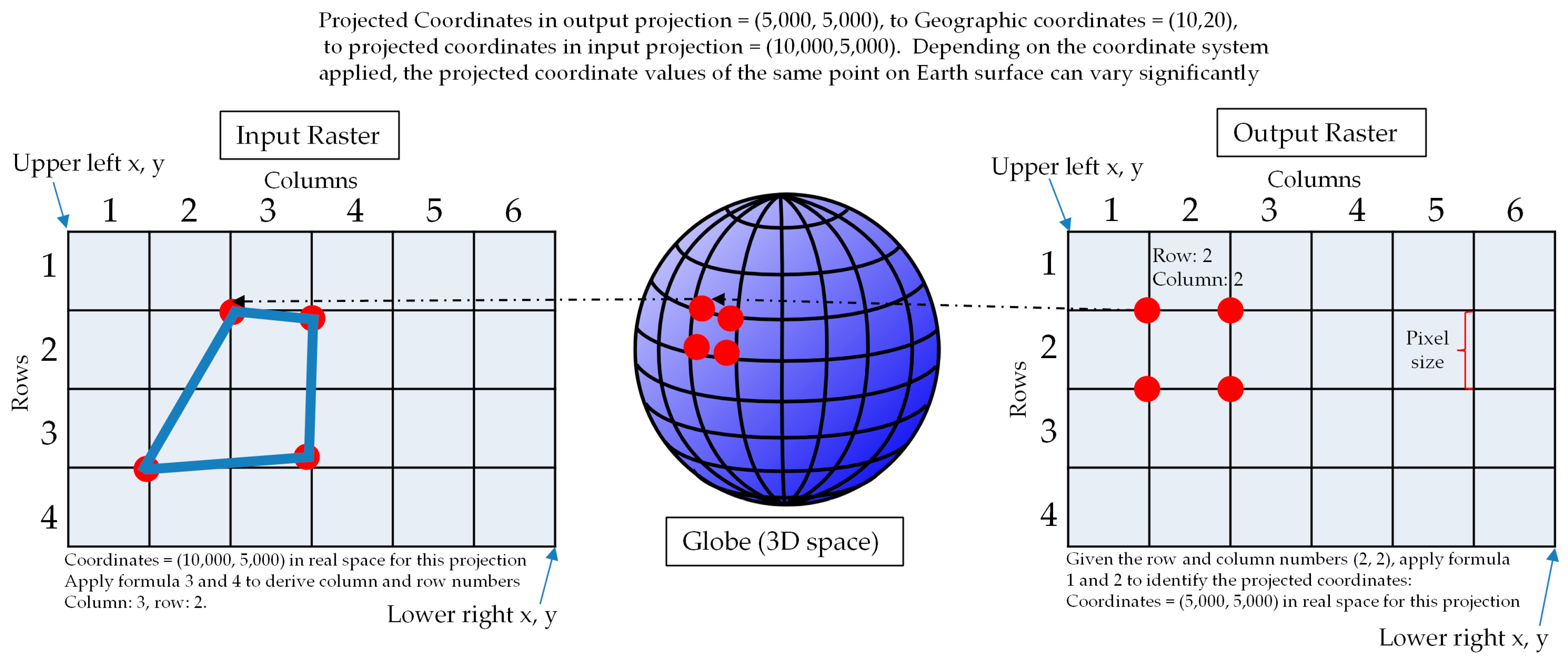
3.1. Rigorous Raster Reprojection in a Serial Processing Manner
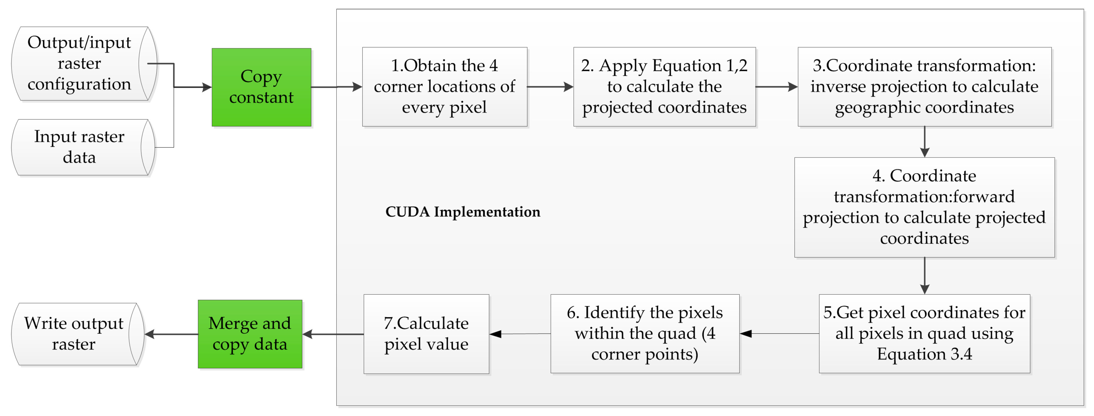
3.2. CUDA-Based Parallel Design and Implementation
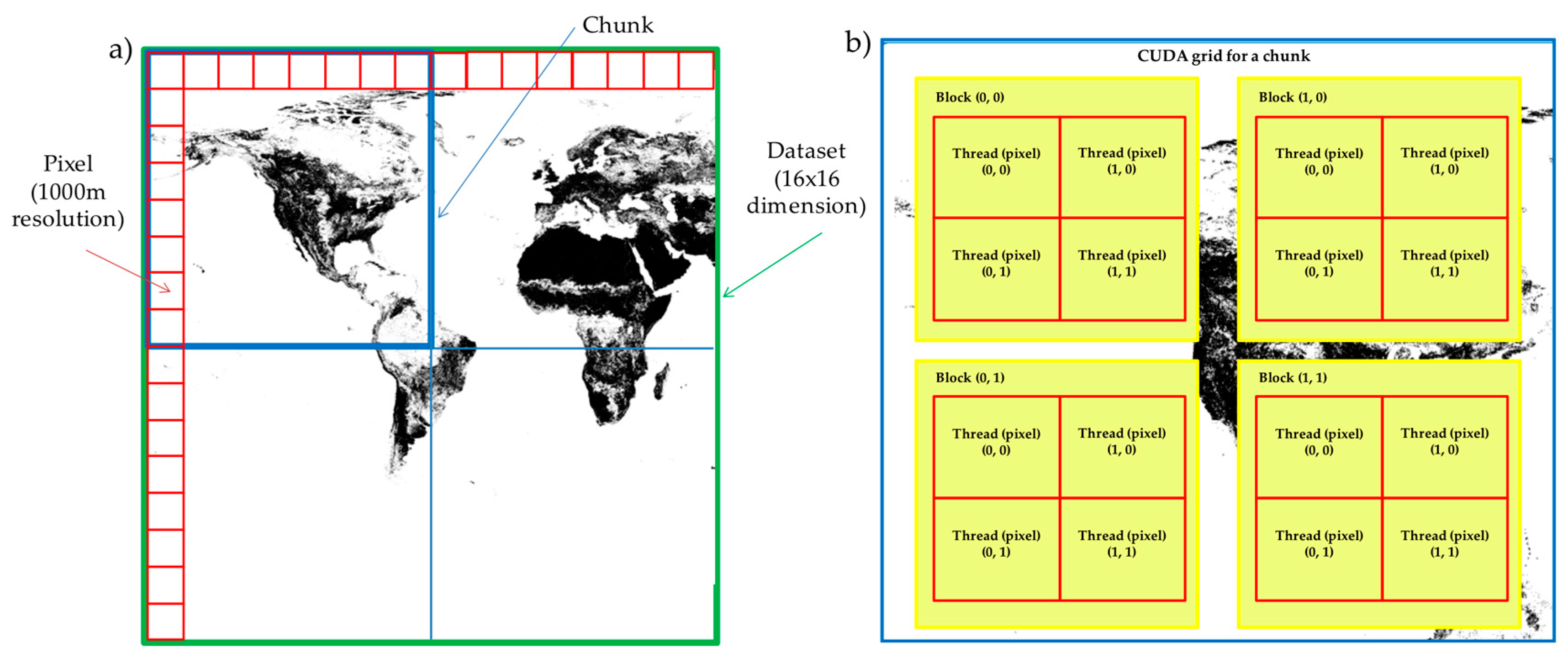
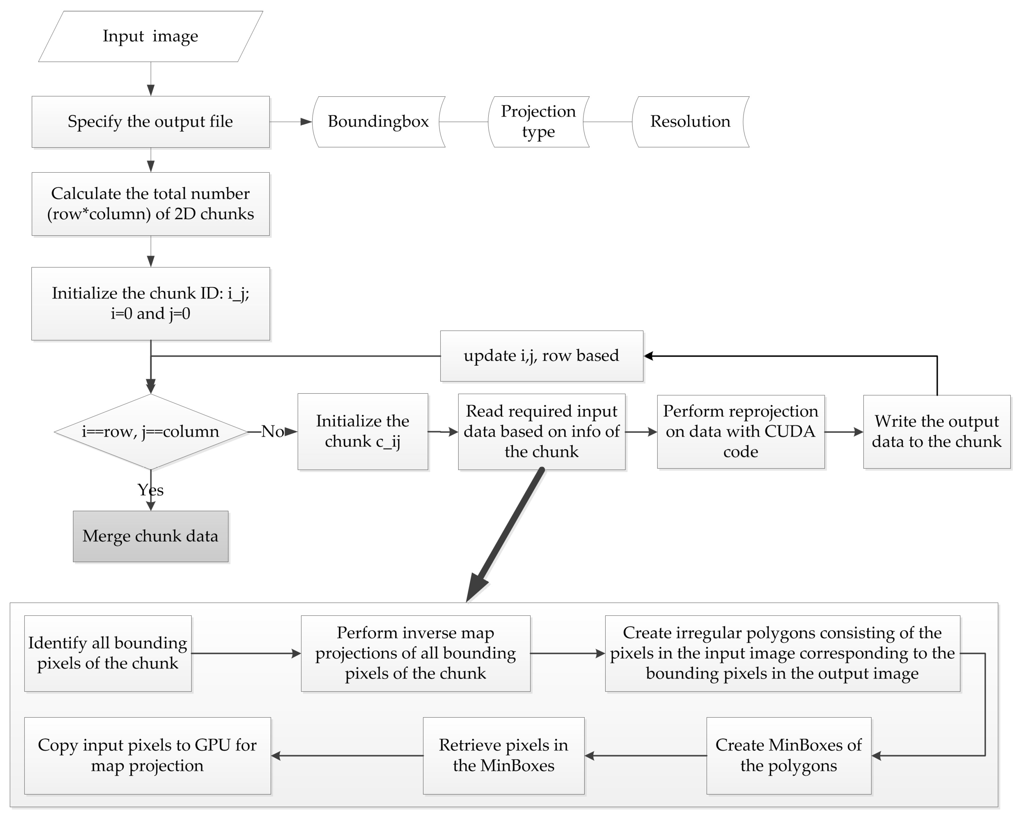
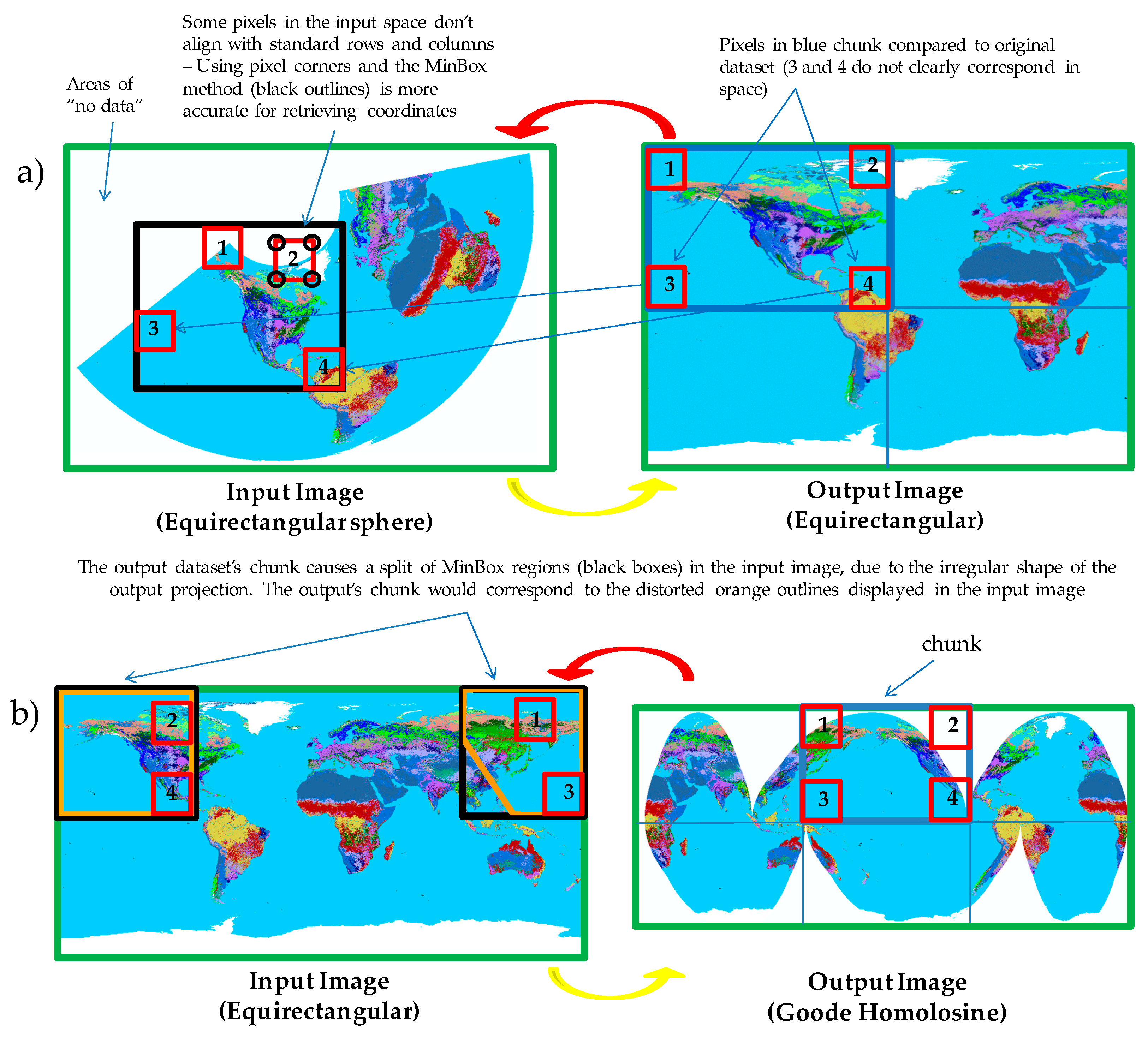
3.3. Handling of Raster Chunks
4. Experiments
4.1. Test Environment
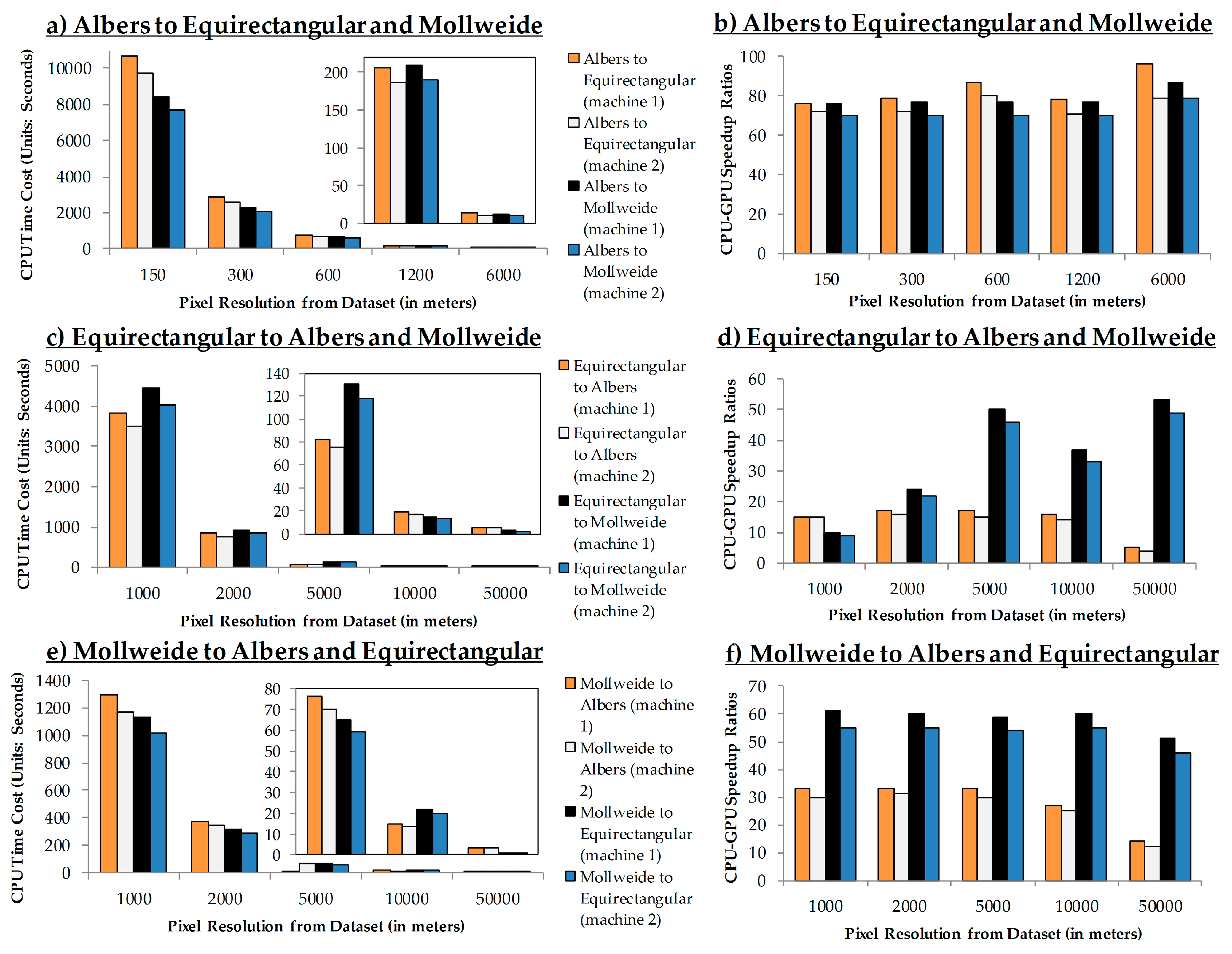
4.2. GPU Speedup Ratios
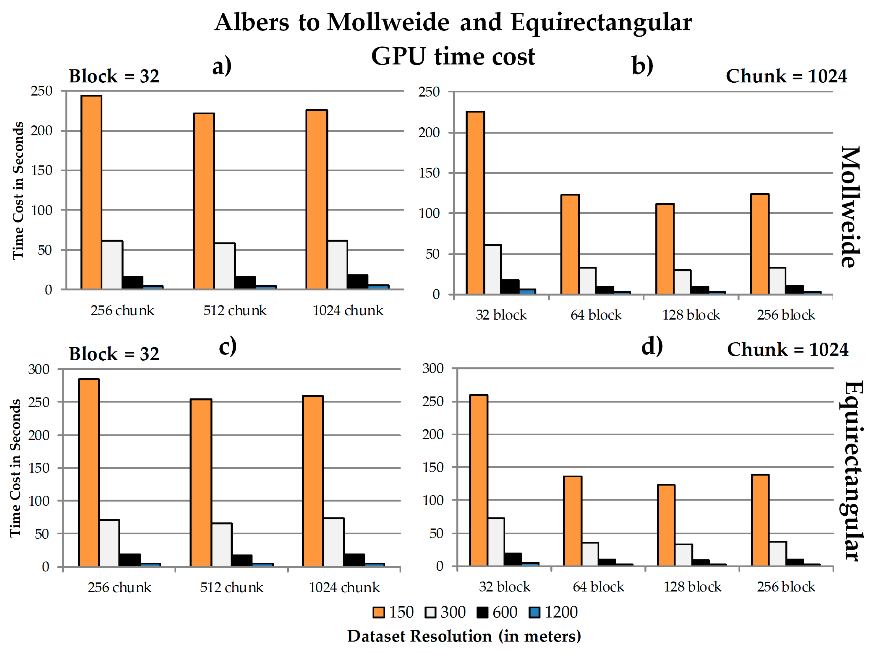
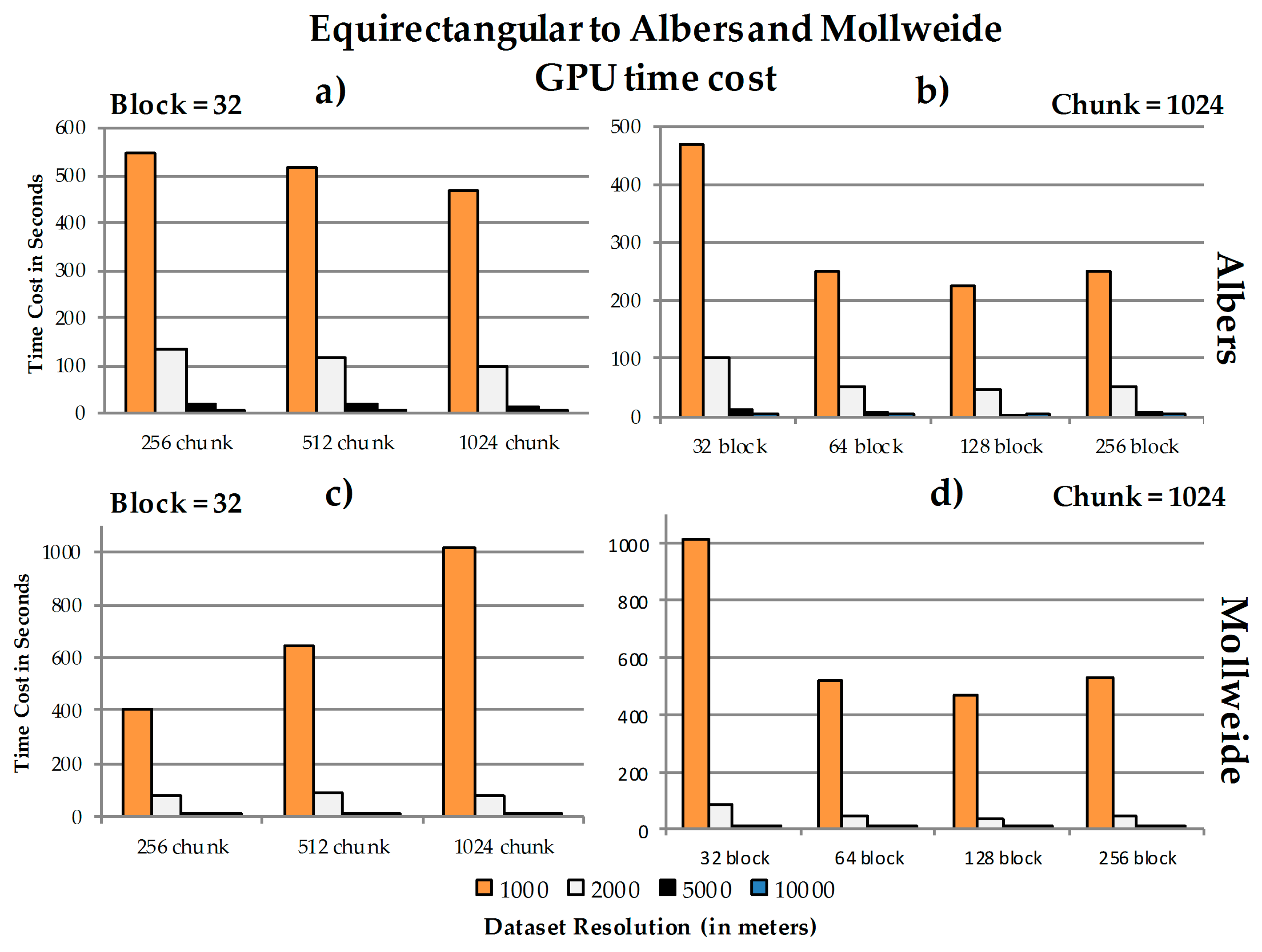
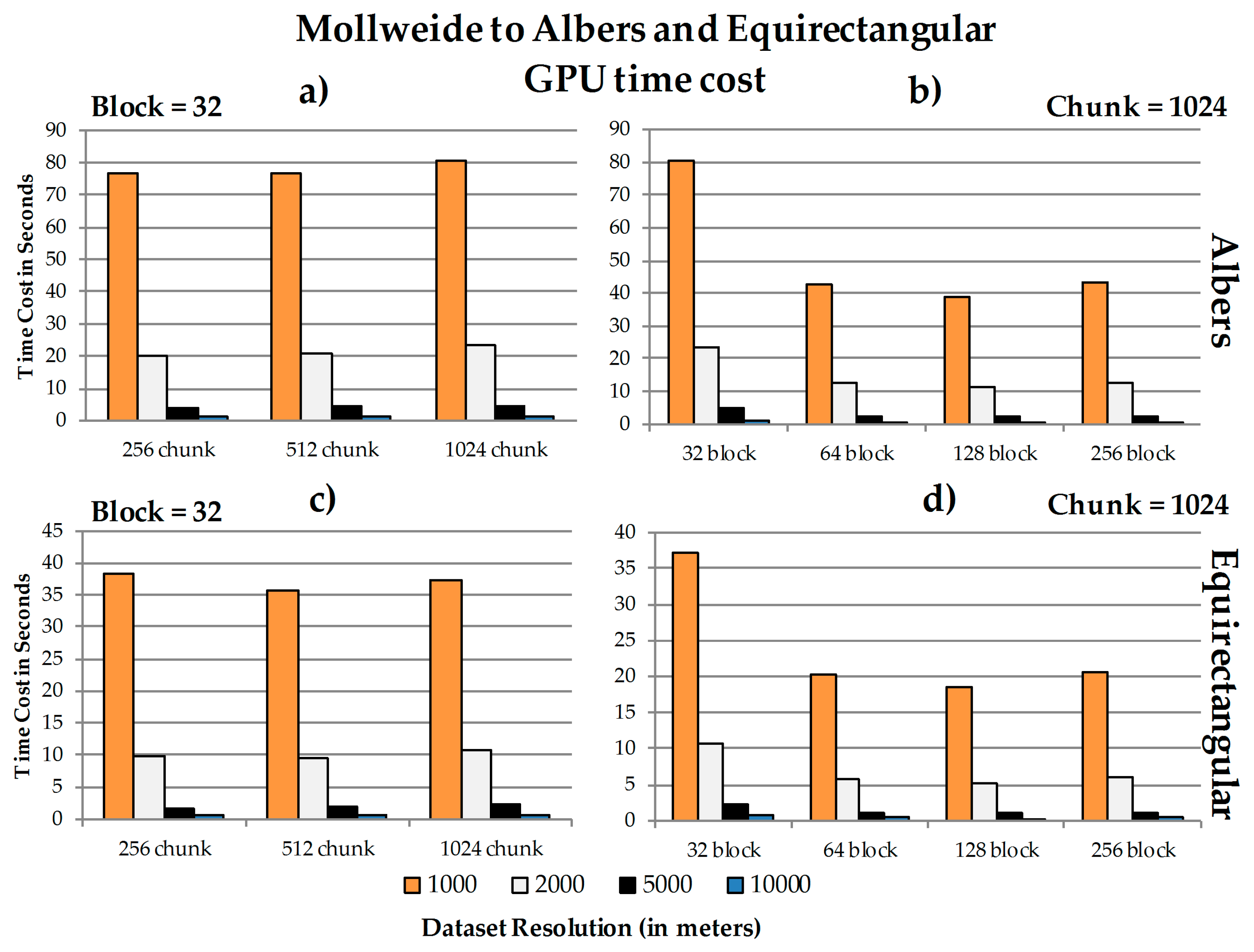
4.3. Data Chunk Size, Spatial Resolution, GPU Block Size, and Performance
4.4. Discussion
4.4.1. Performance
a. GPU speedup ratios
b. The relationship between chunk size, block size and spatial resolution concerning the speedup ratios
4.4.2. Issues
5. Conclusions
Acknowledgments
Author Contributions
Conflicts of Interest
Disclaimer
References
- Wang, S. A CyberGIS Framework for the Synthesis of Cyberinfrastructure, GIS, and Spatial Analysis. Ann. Assoc. Am. Geogr. 2010, 100, 535–557. [Google Scholar] [CrossRef]
- NVIDIA Corporation. Compute Unified Device Architecture (CUDA). Available online: http://www.nvidia.com/object/cuda_home_new.html (accessed on 10 January 2017).
- Bakhoda, A.; Yuan, G.L.; Fung, W.W.L.; Wong, H.; Aamodt, T.M. Analyzing CUDA Workloads Using a Detailed GPU Simulator. In Proceedings of the IEEE International Symposium on Performance Analysis of Systems and Software, Boston, MA, USA, 26–28 April 2009; pp. 163–174. [Google Scholar]
- Finn, M.P.; Steinwand, D.R.; Buehler, R.A.; Mattli, D.; Yamamoto, K.H. A Program for Handling Map Reprojections of Small Scale Geospatial Raster Data. Cartogr. Perspect. 2012, 71, 53–67. [Google Scholar] [CrossRef]
- Beynon, M.; Chang, C.; Catalyurek, U.; Kurc, T.; Sussman, A.; Andrade, H.; Ferreira, R.; Saltz, J. Processing Large-Scale Multi-Dimensional Data in Parallel and Distributed Environments. Parallel Comput. 2002, 28, 827–859. [Google Scholar] [CrossRef]
- Peng, C.; Sandip, S.; Rushing, J. A GPU-accelerated approach for feature tracking in time-varying imagery datasets. IEEE Trans. Vis. Comput. Graph. 2016. [Google Scholar] [CrossRef] [PubMed]
- Tobler, W.R. Polycylindric Map Reprojections. Am. Cartogr. 1986, 13, 117–120. [Google Scholar] [CrossRef]
- Tobler, W.R. Measuring the Similarity of Map Reprojections. Am. Cartogr. 1986, 13, 135–139. [Google Scholar] [CrossRef]
- Usery, E.L.; Seong, J.C. A Comparison of Equal-Area Map Reprojections for Regional and Global Raster Data. Center of Excellence for Geospatial Information Science, 2000. Available online: https://cegis.usgs.gov/reprojection/pdf/nmdrs.usery.prn.pdf (accessed on 10 December 2016).
- Mulcahy, K.A. Two New Metrics for Evaluating Pixel-Based Change in Data Sets of Global Extent Due to Reprojection Transformation. Cartographica 2013, 37, 1–11. [Google Scholar] [CrossRef]
- Usery, E.L.; Finn, M.P.; Coz, J.D.; Beard, T.; Ruhl, S.; Bearden, M. Projecting Global Datasets to Achieve Equal Areas. Cartogr. Geogr. Inf. Sci. 2003, 30, 69–79. [Google Scholar] [CrossRef]
- Finn, M.P.; Trent, J.R.; Buehler, R.A. Users Guide for MapIMG 2: Map Image Re-Reprojection Software Package; U.S. Geological Survey Open-File Report Series; U.S. Geological Survey: Reston, VA, USA, 2006.
- Behzad, B.; Liu, Y.; Shook, E.; Finn, M.P.; Mattli, D.M.; Wang, S. A Performance Profiling Strategy for High-Performance Map Re-Reprojection of Coarse-Scale Spatial Raster Data. In Proceedings of the Auto Carto 2012, A Cartography and Geographic Information Society Research Symposium, Columbus, OH, USA, 16–18 September 2012. [Google Scholar]
- Qin, C.Z.; Zhan, L.J.; Zhu, A.X. How to Apply the Geospatial Data Abstraction Library (GDAL) Properly to Parallel Geospatial Raster I/O? Trans. GIS. 2014, 18, 950–957. [Google Scholar] [CrossRef]
- Atkins, D.; Droegemeier, L.; Feldman, S.; Garcia-Molina, H.; Klein, M.; Messerschmitt, D.; Messina, P.; Ostriker, J.; Wright, M. Revolutionizing Science and Engineering through Cyberinfrastructure: Report of the National Science Foundation Blue-Ribbon Advisory Panel on Cyberinfrastructure; National Science Foundation: Arlington, VA, USA, 2003. [Google Scholar]
- Baumann, P.; Mazzetti, P.; Ungar, J.; Barbera, R.; Barboni, D.; Beccati, A.; Bigagli, L.; Boldrini, E.; Bruno, R.; Calanducci, A.; et al. Big Data Analytics for Earth Sciences: the EarthServer Approach. Int. J. Digit. Earth 2016, 9, 3–29. [Google Scholar] [CrossRef]
- Yang, C.; Huang, Q.; Li, Z.; Liu, K.; Hu, F. Big Data and Cloud Computing: Innovation Opportunities and Challenges. Int. J. Digit. Earth 2016. [Google Scholar] [CrossRef]
- Yang, C.; Manzhu, Y.; Fei, H.; Yongyao, J.; Yun, L. Utilizing Cloud Computing to Address Big Geospatial Data Challenges. Comput. Environ. Urban Syst. 2016. [Google Scholar] [CrossRef]
- Culler, D.E.; Gupta, A.; Singh, J.P. Parallel Computer Architecture: A Hardware/Software Approach; Morgan Kaufmann Publishers Inc.: San Francisco, CA, USA, 1997. [Google Scholar]
- Hennessy, J.; Patterson, D. Computer Architecture: A Quantitative Approach, 4th ed.; Morgan Kauffman: San Francisco, CA, USA, 2007. [Google Scholar]
- Finn, M.P.; Liu, Y.; Mattli, D.M.; Guan, Q.; Yamamoto, K.H.; Shook, E.; Behzad, B. pRasterBlaster: High-Performance Small-Scale Raster Map Reprojection Transformation Using the Extreme Science and Engineering Discovery Environment. In Proceedings of the 22 International Society for Photogrammetry & Remote Sensing Congress, Melbourne, Australia, 25 August–1 September 2012. [Google Scholar]
- Li, J.; Jiang, Y.; Yang, C.; Huang, Q.; Rice, M. Visualizing 3D/4D Environmental Data Using Many-Core Graphics Processing Units (GPUs) and Multi-Core Central Processing Units (CPUs). Comput. Geosci. 2013, 59, 78–89. [Google Scholar] [CrossRef]
- Lukač, N.; Žalik, B. GPU-based roofs’ solar potential estimation using LiDAR data. Comput. Geosci. 2013, 52, 34–41. [Google Scholar] [CrossRef]
- Ortega, L.; Rueda, A. Parallel Drainage Network Computation on CUDA. Comput. Geosci. 2010, 36, 171–178. [Google Scholar] [CrossRef]
- Tang, W.; Feng, W. Parallel Map Reprojection of Vector-Based Big Spatial Data: Coupling Cloud Computing with Graphics Processing Units. Comput. Environ. Urban Syst. 2014. [Google Scholar] [CrossRef]
- Ryoo, S.; Rodrigues, C.I.; Baghsorkhi, S.S.; Stone, S.S.; Kirk, D.B.; Hwu, W.M.W. Optimization Principles and Application Performance Evaluation of a Multithreaded GPU Using CUDA. In Proceedings of the 13th ACM SIGPLAN Symposium on Principles and Practice of Parallel Programming, Salt Lake City, UT, USA, 20–23 February 2008; pp. 73–82. [Google Scholar]
- Steinwand, D.R.; Hutchinson, J.A.; Snyder, J.P. Map Reprojections for Global and Continental Data Sets and an Analysis of Pixel Distortion Caused by Rereprojection. Photogramm. Eng. Remote Sen. 1995, 12, 1487–1497. [Google Scholar]
- Steinwand, D.R. A New Approach to Categorical Resampling. In Proceedings of the American Congress on Surveying and Mapping Spring Conference, Phoenix, AZ, USA, 29 March–2 April 2003. [Google Scholar]
- Snyder, J.P. Map Projections: A Working Manual; U.S. Government Printing Office: Washington, DC, USA, 1987.
- Finn, M.P.; Liu, Y.; Mattli, D.M.; Behzad, B.; Yamamoto, K.H.; Guan, Q.; Shook, E.; Padmanabhan, A.; Stramel, M.; Wang, S. High-Performance Small-Scale Raster Map Reprojection Transformation on Cyberinfrastructure; Future Publication in CyberGIS: Fostering a New Wave of Geospatial Discovery and Innovation; Wang, S., Goodchild, M.F., Eds.; Springer: New York, USA, 2013. [Google Scholar]


| Example Image | Projection | Resampled Dataset Resolution (in meters) | Raster Grid Size (rows by columns) | Description |
|---|---|---|---|---|
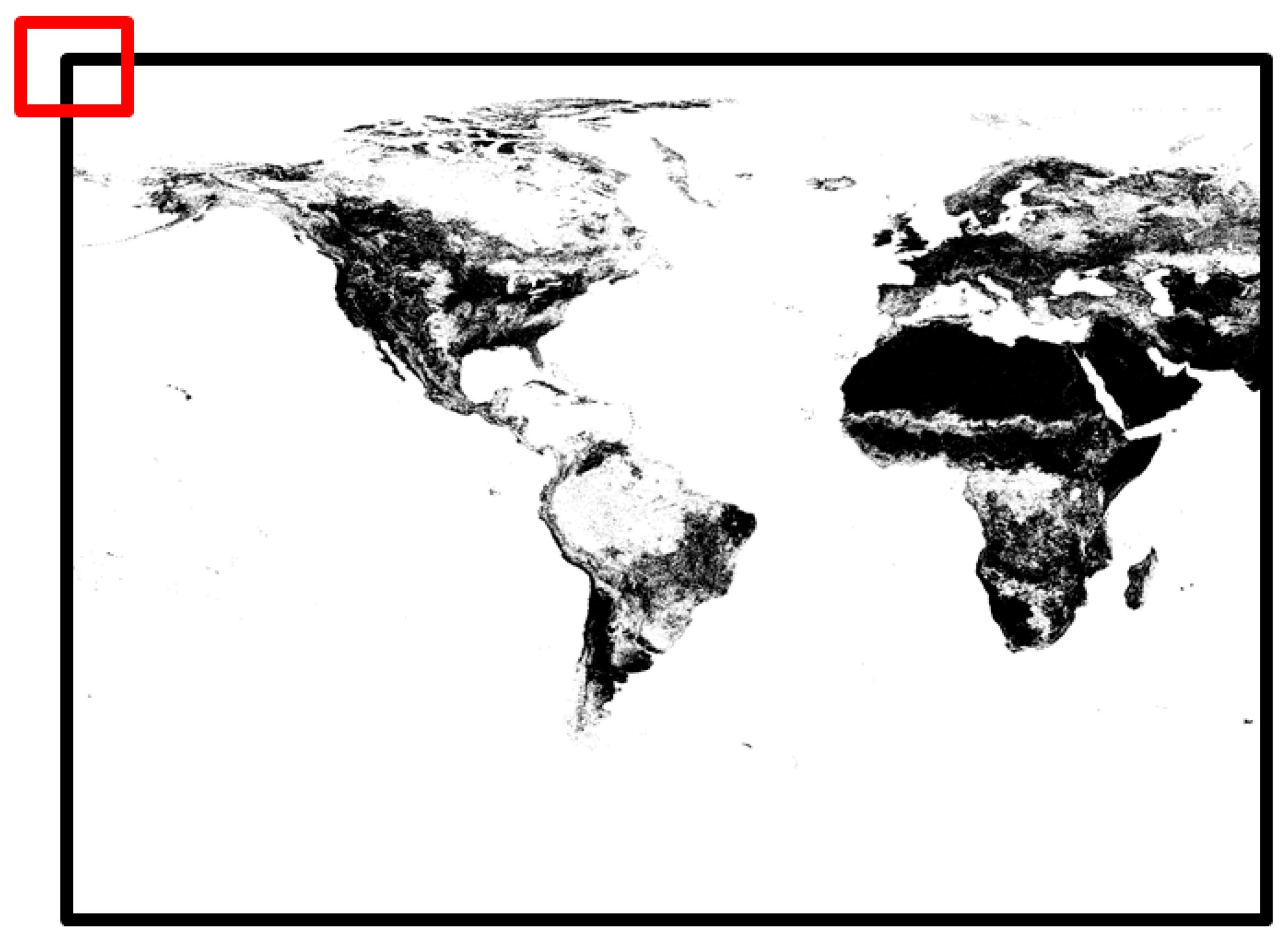
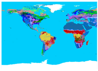 | Equirectangular | 1000 | 28,030 × 20,015 | This dataset covers most of the world and shows different land cover types across the globe. |
| 2000 | 14,015 × 10,008 | |||
| 5000 | 5606 × 4003 | |||
| 10,000 | 2803 × 2002 | |||
| 50,000 | 560 × 400 | |||
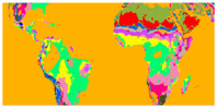 | Mollweide | 1000 | 18,039 × 8021 | This dataset covers areas near the equator on the globe and displays either land cover types or life zone types. |
| 2000 | 9019 × 4010 | |||
| 5000 | 3608 × 1604 | |||
| 10,000 | 1804 × 802 | |||
| 50,000 | 361 × 162 | |||
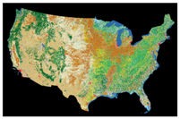 | Albers | 150 | 32,238 × 20,885 | This dataset covers the entire contiguous United States and shows different land cover types across the area. |
| 300 | 16,119 × 10,442 | |||
| 600 | 8060 × 5221 | |||
| 1200 | 4030 × 2611 | |||
| 6000 | 806 × 522 |
| Machine Information | Machine 1 | Machine 2 |
|---|---|---|
| CPU | Intel Quad-core i5 3.10 GHz | Intel Quad-core i7 3.40 GHz |
| Main memory | 8 GB | 8 GB |
| GPU | NVIDIA GeForce GT 640, 384 GPU Cores 1 GB Memory | NVIDIA GeForce GT 640, 384 GPU Cores 1 GB Memory |
© 2017 by the authors. Licensee MDPI, Basel, Switzerland. This article is an open access article distributed under the terms and conditions of the Creative Commons Attribution (CC BY) license (http://creativecommons.org/licenses/by/4.0/).
Share and Cite
Li, J.; Finn, M.P.; Blanco Castano, M. A Lightweight CUDA-Based Parallel Map Reprojection Method for Raster Datasets of Continental to Global Extent. ISPRS Int. J. Geo-Inf. 2017, 6, 92. https://doi.org/10.3390/ijgi6040092
Li J, Finn MP, Blanco Castano M. A Lightweight CUDA-Based Parallel Map Reprojection Method for Raster Datasets of Continental to Global Extent. ISPRS International Journal of Geo-Information. 2017; 6(4):92. https://doi.org/10.3390/ijgi6040092
Chicago/Turabian StyleLi, Jing, Michael P. Finn, and Marta Blanco Castano. 2017. "A Lightweight CUDA-Based Parallel Map Reprojection Method for Raster Datasets of Continental to Global Extent" ISPRS International Journal of Geo-Information 6, no. 4: 92. https://doi.org/10.3390/ijgi6040092
APA StyleLi, J., Finn, M. P., & Blanco Castano, M. (2017). A Lightweight CUDA-Based Parallel Map Reprojection Method for Raster Datasets of Continental to Global Extent. ISPRS International Journal of Geo-Information, 6(4), 92. https://doi.org/10.3390/ijgi6040092