Article

Linking Neighborhood Characteristics and Drug-Related Police Interventions: A Bayesian Spatial Analysis

1
Department of Social Psychology, University of Valencia, Avda. Blasco Ibáñez, 21, 46010 Valencia, Spain
2
Department of Statistics and Operations Research, University of Valencia, Dr. Moliner, 50, Burjassot, 46100 Valencia, Spain
*
Author to whom correspondence should be addressed.
ISPRS Int. J. Geo-Inf. 2017, 6(3), 65; https://doi.org/10.3390/ijgi6030065
Submission received: 15 December 2016 / Revised: 8 February 2017 / Accepted: 21 February 2017 / Published: 25 February 2017
(This article belongs to the Special Issue Frontiers in Spatial and Spatiotemporal Crime Analytics)

Abstract

:
This paper aimed to analyze the spatial distribution of drug-related police interventions and the neighborhood characteristics influencing these spatial patterns. To this end, police officers ranked each census block group in Valencia, Spain (N = 552), providing an index of drug-related police interventions. Data from the City Statistics Office and observational variables were used to analyze neighborhood characteristics. Distance to the police station was used as the control variable. A Bayesian ecological analysis was performed with a spatial beta regression model. Results indicated that high physical decay, low socioeconomic status, and high immigrant concentration were associated with high levels of drug-related police interventions after adjustment for distance to the police station. Results illustrate the importance of a spatial approach to understanding crime.

1. Introduction

The association between crime and place is one of the long-standing topics in the study of crime. From a social disorganization framework, neighborhoods characterized by poverty, ethnic heterogeneity, and residential instability are expected to have higher crime rates [1,2,3]. From this perspective, crime is not randomly distributed in the city; rather, people living in poor and deteriorated neighborhoods are more likely to be the victims of crime [2,4].
Studies based on the social disorganization perspective have largely shown the association of neighborhood concentrated disadvantage, immigration, and residential instability with crime and violence. Concentrated disadvantage reflects the negative socioeconomic features of a neighborhood, such as poverty, unemployment, low income, family disruption, or physical and social disorder [5,6,7]. Research has found that concentrated disadvantage is the factor most strongly associated with crime, even after controlling for individual characteristics [1,8]. Immigration has also been related to crime rates, and previous research has shown that higher levels of ethnic heterogeneity are related to higher levels of crime [1,9,10]. Residential instability is also a relevant factor in social disorganization theory. Studies have found that low residential stability would be related to crime, and neighborhoods with more stable populations should have lower crime rates than those characterized by transitory and changing neighbors [3,11].
It has been suggested that the link between neighborhood characteristics and crime may be mediated by underlying social processes. High levels of social disorganization and concentrated disadvantage in communities would be linked to low levels of social control and collective efficacy. Collective efficacy is defined as ‘the process of activating or converting social ties among neighborhood residents in order to achieve collective goals, such as public order or the control of crime’ [12] (p. 802). A lack of collective efficacy is associated with increased mistrust between neighbors, which creates a dangerous environment and impedes effective social control, thus leading to increased conflict and crime [1,2,5].
The relationship between crime and place has been studied for different types of crime. Most research has focused on residential burglary [13,14,15], juvenile delinquency [16,17], homicides [1,18,19], and robbery and assaults [18,19]. Interest is also growing in studying this relationship in other crimes that tends to occur ‘behind closed doors’ [20] such as intimate partner violence [9,10] or child maltreatment [21].
Drug-related crime has also been linked to neighborhood characteristics [22,23,24]. Drug-related crime is a major problem in our society; it has negative repercussions on health, creates personal and social conflicts, and can perpetuate community deterioration [24,25]. Moreover, some studies have found a relationship between drug dealing and consumption and other types of criminal acts [26]. However, the study of drug-related crime has focused mainly on drug markets [27], and other perspectives and research approaches have received little research attention.
In this study, we aimed to analyze the relationship between neighborhood characteristics and drug-related police interventions from a Bayesian spatial perspective. Clearly, understanding how drug-related police interventions are spatially distributed across a city’s neighborhoods and how they relate to neighborhood characteristics may contribute to preventing this type of crime and related negative outcomes in the community.
Recently, research linking crime and neighborhood characteristics has relied more heavily on spatial analysis [9,10,28,29]. The majority of these studies use the frequentist or classical paradigm [30]. However, recent research is showing the advantages of using spatial methods from a Bayesian perspective [9,10,29]. These types of models come from disease mapping [31] and are increasingly being incorporated into social studies [9,10,29]. The frequentist approach treats parameters as fixed unknown values, while the Bayesian approach uses probability distributions to represent the uncertainty of the parameters [32]. Researchers may base their interpretation of this probability on their knowledge about the parameters, and it allows random effects to be included. Including random effects reduces the biases of spatial autocorrelation and overdispersion common in spatial analysis [33]. In addition, Bayesian models provide risk estimations and analyze the effect of unobserved spatially structured influences [34,35]. The use of a Bayesian spatial random-effects modeling approach in this study (almost nonexistent in current research) may provide new knowledge and a new perspective to research on drug-related crime [36,37]. Most studies focusing on drug crime and place have been conducted in Anglo-Saxon cities (predominantly in the US, UK, or Australia). However, there are fewer studies from other European areas such as Southern European cities. Analyzing drug-related crimes in cities from different countries would add new valuable data to the existing literature.

2. Study Area and Data

In this study, we conduct a Bayesian ecological analysis to understand the influence of neighborhood characteristics on the spatial distribution of drug-related police interventions. Ecological studies are based on populations that are defined geographically. Following a social disorganization perspective, we analyze the influence of four neighborhood-level variables; two different measures of concentrated disadvantage (socioeconomic status and physical decay), immigrant concentration, and residential instability. We also consider that the proximity of the police station could also have a deterrent effect, and therefore we include the distance to the nearest police station as a control variable.

2.1. Study Area

This study was conducted in Valencia, the third largest city in Spain, which has a population of 736,580 inhabitants and covers an area of 134 km2 approximately. Its fairly large size allows us to study the spatial distribution with adequate variability.
We used the census block group as a proxy for neighborhood. Census block groups were the smallest administrative units available, and they are defined as walkable areas with a low number of city blocks and are smaller than a census tract [9,10,38]. The sample had 552 census block groups with an average of 1334 residents (a maximum of 2845 and a minimum of 630).

2.2. Dependent Variable

To study drug-related crimes, we used the police perception of the level of drug interventions conducted in each census block group. Police records have been used extensively to study crime [9,10,30] but they were not available for this study. However, previous research suggests that police perception and police records are correlated for some types of crime [39]. In the present study, we use police perceptions of police interventions. With this measure, we can distinguish between areas where the police intervene more frequently from those with a low level of interventions. In this way, we capture all the police’s valuable experience and information [39,40]. Police perceptions could be especially useful to study under-reported crime, and they could help to plan law enforcement policies or urban planning strategies.
Senior police officers with a thorough knowledge of the area were selected to provide an index of policing activity, indicative of the level of drug-related crime in each census block group (i.e., they evaluated the level of police interventions where drugs are involved). This index was based on police officers’ perceptions and experience. Police officers placed each census block group on a 5-interval scale, in which the first interval represented a very low level of drug-related interventions and the fifth interval, a very high level of drug-related interventions.

2.3. Independent Variables

In this study we used data provided by the City Statistics Office and observation data gathered by trained raters; all data corresponded to 2013.
Socioeconomic Status (SES): We constructed an index using several socioeconomic indicators, as in previous research [10]. These indicators showed a high correlation, and a scale was created through factor analysis to avoid collinearity. The scale consisted of the following variables: (a) cadastral value, an administrative value of a property calculated by the city council and used as a reference for fiscal and other administrative purposes; (b) percentage of high-end cars; (c) percentage of financial businesses (percentage of financial institutions and insurance companies out of total activities); (d) percentage of commercial businesses (percentage of trade, hostelry, or repairs business out of total activities); and (e) education level, measured on a 4-point scale, where 1 = less than primary education, 2 = primary education, 3 = secondary education, and 4 = college education. We selected the first principal component of the factor analysis in which the five variables had a relevant factorial weight (i.e., each variable was properly represented in the scale).
Observed Physical Decay: Trained raters assessed the level of observable physical decay in each census block group. A 4-item scale was used including the following items: vacant houses; abandoned, vandalized and run-down buildings; deteriorated residential units; and deteriorated recreation places [38]. Each item was rated from 0 to 4, where 0 indicates no presence and 4 indicates high presence. Observations were made during business hours.
Immigrant Concentration: Percentage of immigrant population in each census block group.
Residential Instability: We used an index of residential mobility, measured as the proportion of the population who had moved into or out of each census block group during the previous year (rate per 1000 inhabitants).
Distance to Police Station: Euclidean distance to police stations was measured to control for the deterrent effect they may have on drug crime. Distance was measured as the kilometers between the centroid of each census block group and the nearest police station.
Table 1 summarizes the descriptive statistics for all the variables.

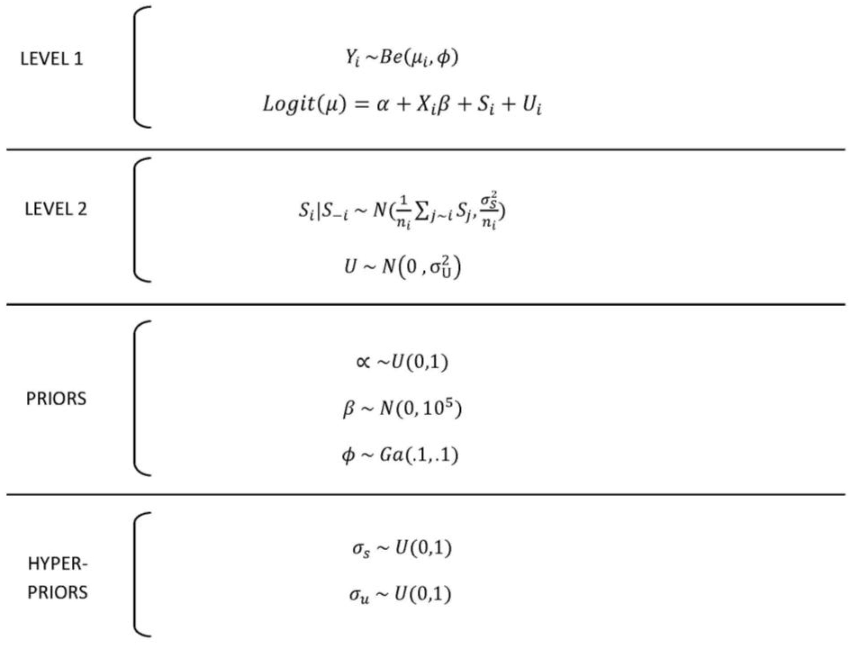
3. Design and Analysis
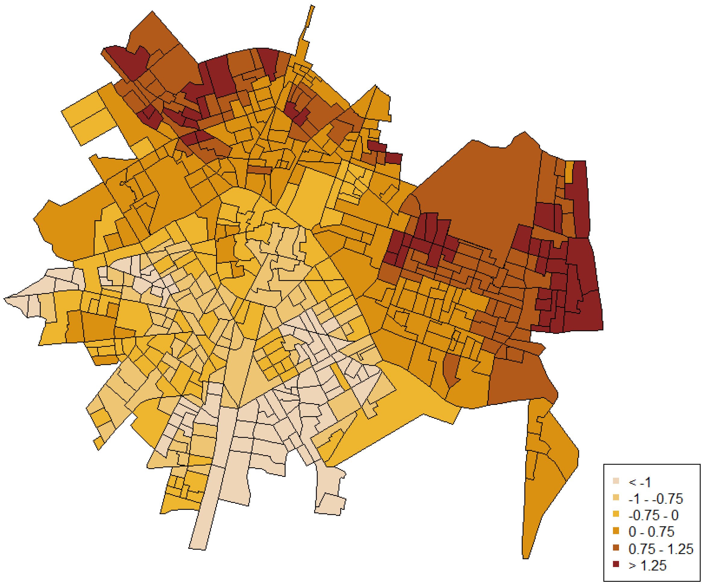
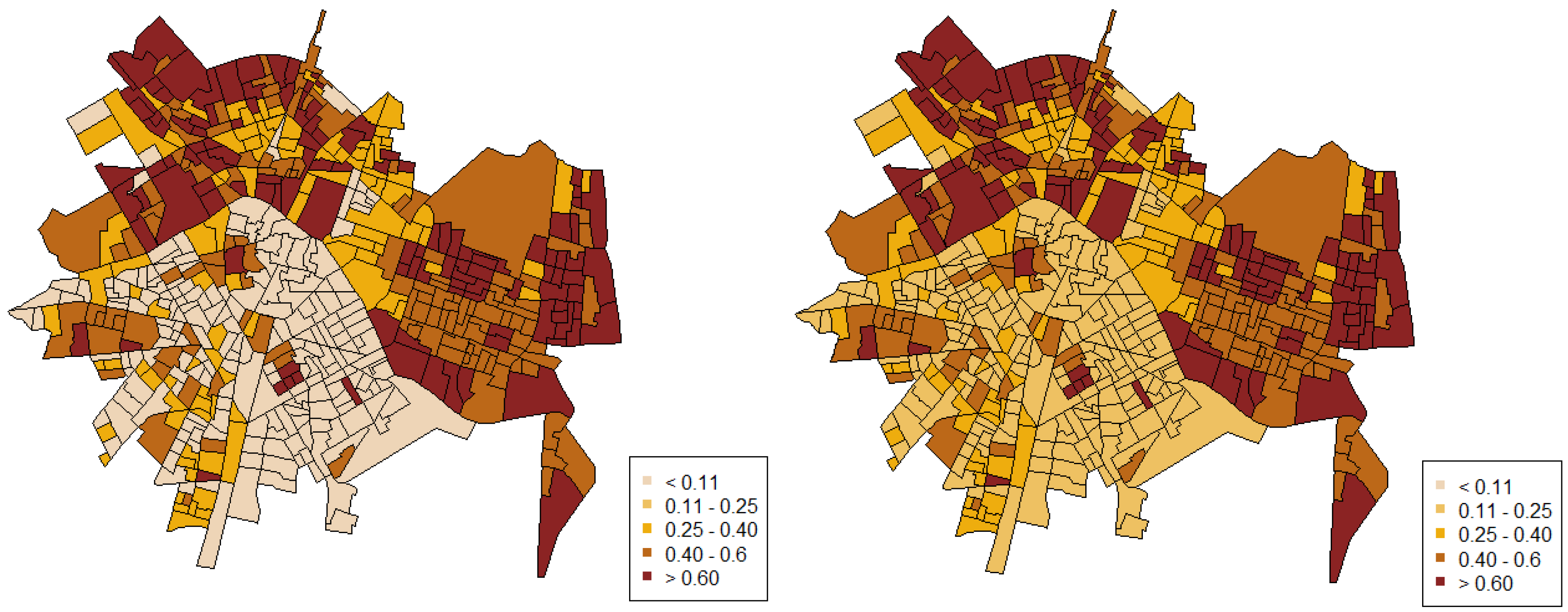
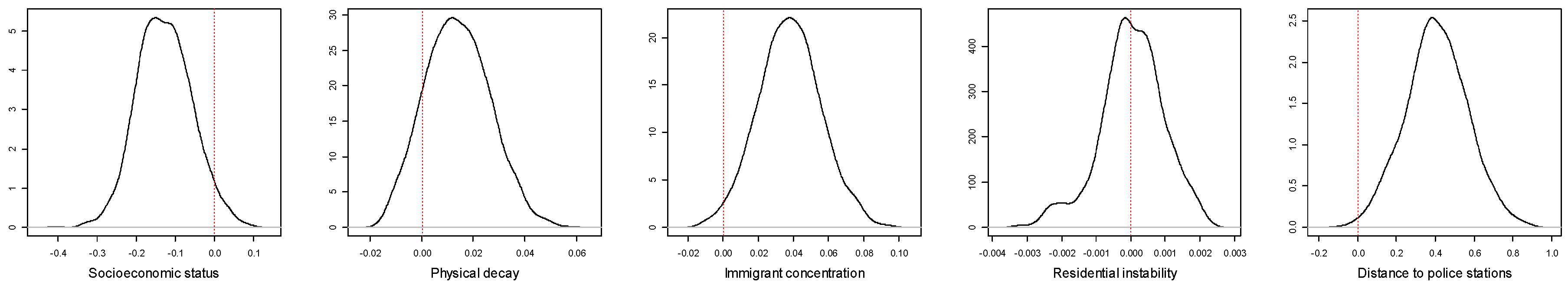
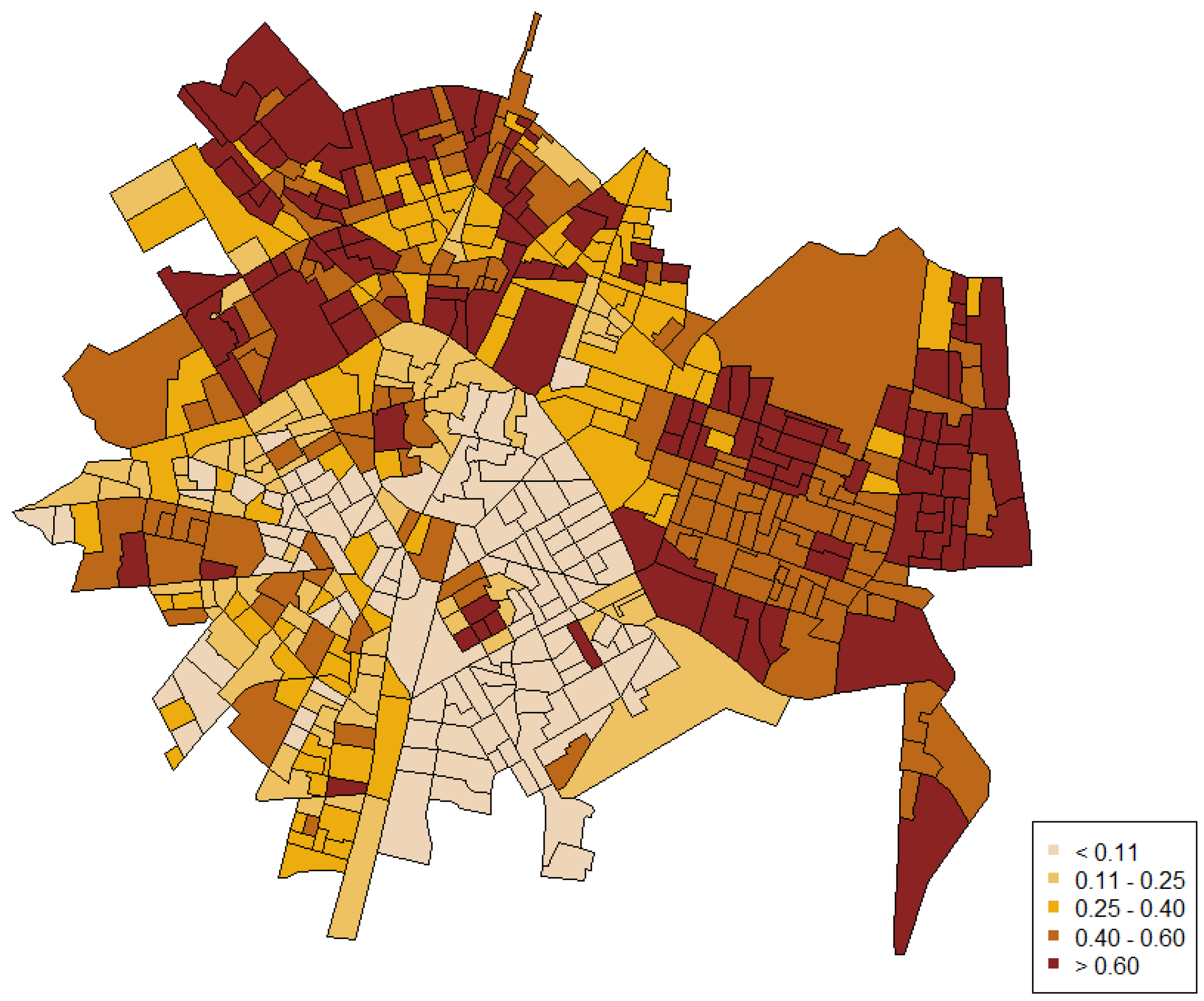
We assumed the dependent variable (an index of the level of drug-related police interventions) as a proportion based on police perception between 0 and 1 on a continuum, where 0 was the minimum perceived level of drug-related police interventions and 1, the maximum perceived level. A value of 0.5 therefore would be the intermediate level of perceived police interventions. We considered that a beta distribution (a continuous positive distribution used with variables bounded between a minimum and a maximum) best reflects the nature of this variable, which is commonly used for modeling proportions [41,42]. Five intervals were established, and we took the average value of each interval. Specifically, if Y i represents the level of interventions, we assumed that Y i ~ B e ( μ i , ϕ ), where μ i is the mean level of interventions in each of the i census block groups and ϕ is a secondary parameter to regulate the variability of the distribution.
We performed regression modeling using Generalized Linear Models with a logit link function. The model assessed included the five explanatory variables; socioeconomic status, immigrant concentration, physical decay, residential instability, and distance to the police station.
A random effect to determine spatial autocorrelation was introduced to account for the spatial effect. Spatial autocorrelation occurs because nearby areas are more related to each other than more distant areas [43]. In social research, this effect may occur because the surrounding areas have similar social, economic, and cultural characteristics [44]. Detecting spatial dependence may be useful to provide information about the spatial structure of the data.
Moreover, an unstructured random effect was included to account for the heterogeneity, overdispersion, and the arbitrariness of spatial unit choice. This effect is related to the spatial differentiation of geographic units, (i.e., when the data are not homogeneous throughout the data set). In these cases, there may be greater variability than expected under the assumed distribution [45]. An unstructured random effect would correct and smooth the distribution [34].
Therefore, the complete model is as follows:
L o g i t ( μ ) = α + X i β + S i + U i
where α is the total mean (intercept), β represents the vector of the regression coefficients, X i is the matrix of covariates in the census block group i ( i = 1 , , n ) , and S i and U i are two random effects terms, which explore spatial autocorrelation and overdispersion respectively.
The component S i is the spatially correlated heterogeneity, and it was specified by a conditional spatial model (CAR). [45]:
S i | S i ~ N ( 1 n i j ~ i S J , σ S 2 n i )
We used contiguity as neighborhood criterion. Contiguity is one of the most common criteria for urban contexts where areas are connected. Thus, adjacent areas were considered neighbors.
The random unstructured heterogeneity ( U i ) was specified as a normal distribution centered at zero with standard deviation σu. The standard deviations of S and U were defined as a prior uniform distribution U ( 0 , 1 ) .
Generalized linear models may be analyzed following a frequentist methodology. However, Bayesian methods introduce random effects and are more flexible. Taking a Bayesian approach, the parameters are treated as random variables, and we need to incorporate prior distributions to assess prior knowledge [45]. In our study, we used vague Gaussian distributions N ( 0 , 100000 ) for the fixed effects β and an improper uniform distribution for α . Finally, we used a Gamma distribution G a ( 0.1 , 0.1 ) to define the prior distribution of ϕ . A sensitivity analysis on these prior distributions was performed to select the most suitable possible prior distributions, repeating the study with different prior distributions values. Specially, we focus on the prior distribution of the variability parameters (σs, σu, and ϕ ). The results did not change using different prior distributions. Figure 1 shows the complete model and the hierarchical structure.
To perform estimations, we generated simulations of the parameters with Markov Chain Monte Carlo (MCMC) using the software R and WinBUGS (see Appendix A for the WinBUGS code for the model). A total of 1,000,000 iterations were carried out (the first 10,000 were discarded as burn-in).
Convergence of the simulated samples was measured using the convergence diagnostic R ^ [46], which was close to 1.0 for all parameters. The posterior distributions showed consistent results. To select the final model, we ranked the deviance information criterion (DIC), and the model with the lowest DIC was chosen because it shows a better fit.

4. Results

A Bayesian beta regression model was conducted with the five explanatory variables (socioeconomic status, immigrant concentration, residential instability, physical decay, and distance to the police station) and two random variables were introduced (unstructured U and structured spatial S effect). The DIC of this model was −1431.8. We ran a second model without these two random variables, and the model fit was clearly the worst (DIC = −190.7). The complete model represented the best fit and was therefore selected as the final model. Table 2 summarizes the results of the final regression model.
The posterior distribution of fixed effects (Figure 2) shows the probability of having a negative or positive association between independent variables and the outcome variable, and it allows us to assess the relevance of the variables in the model. Variables with a posterior probability of being different from zero above 80% were considered relevant to the outcome variable. Specifically, socioeconomic status has a 96% probability of having a negative association, and immigrant concentration, physical decay and distance to the police stations have a high probability of having a positive association (87.3%, 98.8% and 99.4% respectively). Residential instability did not have a clear association with drug-related police interventions (only a 53.6% probability of having a positive association). Thus, areas with lower socioeconomic status, high levels of immigrant concentration, and high physical decay and that are further from police stations showed higher mean levels of drug-related police interventions.
Beyond the effect of the variables, the results showed the influence of spatial dependency and unstructured heterogeneity. A Bayesian approach reveals the spatial effect through illustrative maps. Figure 3 shows the posterior mean value for the spatial component. There is a clear geographic pattern: northern areas of the city have higher mean values than southern areas. This indicates the existence of a significant underlying spatial process that is not explained by the variables we have explored.
Figure 4 shows the mean level of drug-related police interventions in each census block group once we incorporated explanatory variables and random effects (heterogeneity and spatial autocorrelation). Some areas have high levels of interventions, and others have very low levels. Specifically, there is a higher probability of drug-related interventions in the northern and eastern zones; some areas have a level of intervention higher than 80%. This map shows the areas with higher mean levels of drug-related police interventions, which is useful when planning and implementing prevention and intervention strategies. Also, to map the uncertainty associated with the posterior means, Figure 5 represents the map of the first and the third quartile for the posterior mean level of drug-related police interventions.

5. Discussion

In this study, we conducted a spatial analysis of drug-related police interventions exploring the influence of neighborhood characteristics. A Bayesian spatial modeling approach was used, which is common in health and epidemiology studies [34] and is especially appropriate to study small-area variations [47]. We used census block groups (the smallest unit available), and, drawing from social disorganization theory, we explored the influence of four neighborhood characteristics; socioeconomic status, physical decay, immigrant concentration, and residential instability. We incorporated distance to the police station in each census block group as a control variable to avoid the confounding effect that it could have on drug-related crime.
Our results showed a significant spatial distribution, according to which the areas with lower levels of socioeconomic status and higher levels of physical decay, higher immigrant concentration, and greater distance to a police station were those which had higher levels of drug-related police interventions. Residential instability, however, was not clearly associated with the distribution of drug-related interventions.
These results are in line with previous research. Social disorganization theory suggests that areas with higher concentrated disadvantage, higher ethnic heterogeneity, and higher residential mobility should show higher levels of disorder and crime [1,3,17]. In order to measure concentrated disadvantage, two indicators were used, both leading to the same results. On the one hand, we measured socioeconomic status, and we observed a negative relationship with drug-related police interventions, as expected from previous literature [48]. The second indicator used was physical decay, which measured the level of structural disorder in the neighborhood. Our results showed that physical decay was positively related to drug-related police interventions, also in line with previous research [26].
With respect to immigrant concentration, we found a positive association with drug-related police interventions. Some studies have shown similar results with other types of crime [1,9,10,49]. However, other studies showed a negative or null association between immigrant concentration and crime when socioeconomic characteristics are controlled for [50,51]. As regards drug-related crime, our results are similar to those found in other studies [52]. It is important to note, however, that most of these studies come from the US, and most of them focus on black residents and the black sub-culture of drugs and violence [11,53]. In Spain, most immigrants are from South American (34.3%) and European (34%) countries. These differences should be taken into account to properly analyze the effect of immigration on drug-related interventions.
Residential instability, however, did not have a significant influence on the spatial distribution of drug-related police interventions. The research is inconclusive on this question; some studies found a positive association between residential instability and crime [8,11], while others found no correlation [9,10,54]. Our study aligns with the second group.
Finally, because we considered that distance to the police station could also have a deterrent effect, we included it as a control variable. We found evidence to support our hypothesis that the places closest to a police station are less likely to be the scene of drug-related crimes. The introduction of this control variable increases the model fit, and without it there could be a confounding effect that is unaccounted for. The distance method available for the study was Euclidean distances. Due to the street distribution of Valencia (a round city, with no important architectural or natural barriers), this type of distance was considered appropriate. However, future research would benefit from taking into account distance-based relationships, which could be a more accurate measure for distances in the context of a city.
Taking these explanatory variables together and analyzing the distribution of the mean level of drug-related police interventions, we can appreciate some important differences among census block groups. Specifically, some areas in the north and the east of the city present higher drug-related police interventions, indicating that police officers perceived that more drug-related police interventions are needed in such areas. These results suggest that police strategy should point to those city areas that show higher perceived drug-related police interventions.
Bayesian statistics have the advantage of incorporating a random effect beyond those explained by the variables considered in the study to explore the underlying spatial distribution in the variable of interest [10,34]. In our study, we found a spatial distribution unexplained by the specific covariates. The drug-related police interventions showed a clear spatial distribution, wherein the estimated prevalence was higher in the north of the city and lower in the south. Future research should consider other variables when attempting to explain this gradient. One possible explanation is that these neighborhoods placed in the north and east of the city may carry the burden of stigma (i.e., deprived neighborhoods historically related to crime and disorder) [55]. The police perceptions on drug-related crime could be influenced by such stigmatization. This hypothesis could be further explored in future studies comparing police calls or police reports data with police perceptions.
This study had both strengths and limitations. One of the strengths is that few studies focus on crime from an epidemiological perspective using Bayesian regression analysis, and there has been little research on drug-related crime [36]. Thus, this study contributes by adding a new approach to the existing literature. Furthermore, Bayesian models allow controlling for biases such as overdispersion and spatial autocorrelation and allow underlying spatial patterns to be analyzed [10,34,35]. Finally, explanatory variables were collected from two different sources, census data and systematic observations, which make the study more complete and provide more information about the neighborhood characteristics.
Among the limitations, the use of a subjective measure of the police perceptions on drug-related crime is a potential shortcoming since there is no numerical value of police interventions on drug-related crimes in small areas. This could be a handicap due to the nature of subjective data. However, previous research suggests that police perception correlates to census data [39,40], and using a subjective police measure could provide additional information to objective data when detecting risk areas [28,39]. Police perceptions, moreover, could be especially adequate to study under-reported crime, and some authors highlight the importance of social perceptions for law enforcement policies or urban planning [55].
Furthermore, some variables that may be relevant to the study of crime [18] were not used in this study. For example, data on collective efficacy and neighborhood processes were not available, as well as variables related to routine activities or crime pattern theory [56,57], which would help to better understand the spatial distribution of drug-related crime. Future research could be enriched by the addition of these variables. Moreover, ecological studies present some biases due to the aggregation of data (e.g., ecological fallacy or the modifiable areal unit problem) [10]. However, this study was conducted with high spatial resolution (census block groups), reducing the ecological biases from aggregation effects.
Lastly, it should be taken into account that this study was conducted in a European city with specific characteristics and its own culture. As noted, most studies are conducted in US cities [58] and there are fewer studies from Europe [30,59]. The differences in the culture and structure of European cities may lead to different results than those from studies conducted in US cities [10,60,61]. However, since our study was conducted in a European city, our results offer a valuable addition to the existing literature, bearing in mind that an understanding of these cultural variables is important to reliably analyze the results.

6. Conclusions

The results of this study illustrate the importance of a spatial and contextual approach to understanding drug-related crimes. A spatial perspective provides a new approach in the study of crime in neighborhoods and could help to improve and design new crime prevention policies at more localized level (e.g., allocating more human and economic resources to those high risk areas, or conducting studies over time to assess the effectiveness of new policies in reducing crime).

Acknowledgments

This research was supported by the Spanish Ministerio de Economía y Competitividad (grant number PSI2014-54561-P). Miriam Marco was supported by the FPU program of the Spanish Ministerio de Educación, Cultura y Deporte (FPU2013/00164). We wish to thank José Serrano, Chief of the Valencia city Police Department, for his support and assistance in collecting the data for this study. Without his enthusiasm and involvement, this study would have not been possible.

Author Contributions

Miriam Marco, Enrique Gracia, and Antonio López-Quílez conceived the study; Miriam Marco prepared data, performed statistical analysis, and wrote the paper; Enrique Gracia analyzed the results and wrote and edited the paper; Antonio López-Quílez supervised the statistical analysis and contributed to writing.

Conflicts of Interest

The authors declare no conflict of interest.

Appendix A. WinBUGS Code

model{
for(i in 1:n) {
y[i] ~ dbeta(a[i], b[i])
a[i] <- mu[i] * phi
b[i] <- (1-mu[i]) * phi
logit(mu[i]) <- alpha + beta[1]*X1[i] + beta[2]*X2[i] + beta[3]*X3[i] + beta[4]*X4[i]+ beta[5]*X5[i] + S[i] + U[i]
U[i] ~ dnorm(0,prec.u)
}
phi ~ dgamma(.1,.1)
S[1:n] ~ car.normal(adj[], weights[], num[],prec.s)
prec.s <- pow(sigma.s,-2)
sigma.s ~ dunif(0,1)
prec.u <- pow(sigma.u,-2)
sigma.u ~ dunif(0,1)
alpha ~ dflat()
for(i in 1:5){
beta[i] ~ dnorm(0, 0.00001)
}
}

References

  1. Sampson, R.J.; Raudenbush, S.W.; Earls, F. Neighborhoods and violent crime: A multilevel study of collective efficacy. Science 1997, 277, 918–924. [Google Scholar] [CrossRef] [PubMed]
  2. Sampson, R.J.; Groves, W.B. Community structure and crime: Testing social-disorganization theory. Am. J. Sociol. 1989, 94, 774–802. [Google Scholar] [CrossRef]
  3. Shaw, C.R.; McKay, H.D. Juvenile Delinquency and Urban Areas; University of Chicago Press: Chicago, IL, USA, 1942. [Google Scholar]
  4. Peterson, R.D.; Krivo, L.J. Segregated spatial locations, race-ethnic composition, and neighborhood violent crime. Ann. Am. Acad. Political Soc. Sci. 2009, 623, 93–107. [Google Scholar] [CrossRef]
  5. Kubrin, C.E.; Weitzer, R. New directions in social disorganization theory. J. Res. Crime Delinq. 2003, 40, 374–402. [Google Scholar] [CrossRef]
  6. Morenoff, J.D.; Sampson, R.J.; Raudenbush, S.W. Neighborhood inequality, collective efficacy, and the spatial dynamics of urban violence. Criminology 2001, 39, 517–558. [Google Scholar] [CrossRef]
  7. Wilson, W.J. The Truly Disadvantaged: The Inner City, the Underclass and Public Policy; University of Chicago Press: Chicago, IL, USA, 1987. [Google Scholar]
  8. Thompson, S.K.; Gartner, R. The spatial distribution and social context of homicide in Toronto’s Neighborhoods. J. Res. Crime Delinq. 2013, 51, 88–118. [Google Scholar] [CrossRef]
  9. Gracia, E.; López-Quílez, A.; Marco, M.; Lladosa, S.; Lila, L. Exploring neighborhood influences on small-area variations in intimate partner violence risk: A Bayesian random-Effects modeling approach. Int. J. Environ. Res. Public Health 2014, 11, 866–882. [Google Scholar] [CrossRef] [PubMed]
  10. Gracia, E.; López-Quílez, A.; Marco, M.; Lladosa, S.; Lila, L. The spatial epidemiology of intimate partner violence: Do neighborhoods matter? Am. J. Epidemiol. 2015, 182, 58–66. [Google Scholar] [CrossRef] [PubMed]
  11. Bursik, R.J., Jr.; Webb, J. Community change and patterns of delinquency. Am. J. Sociol. 1982, 88, 24–42. [Google Scholar] [CrossRef]
  12. Sampson, R.J. Collective efficacy theory. In Encyclopedia of Criminological Theory; Cullen, F.T., Wilcox, P., Eds.; SAGE: Thousand Oaks, CA, USA, 2010; pp. 802–812. [Google Scholar]
  13. Townsley, N.; Homel, R.; Chaseling, J. Repeat burglary victimization: Spatial and temporal patterns. Aust. N. Z. J. Criminol. 2000, 33, 37–63. [Google Scholar] [CrossRef]
  14. Johnson, S.D.; Bowers, K.J. The stability of space-time clusters of burglary. Eur. J. Criminol. 2005, 2, 67–92. [Google Scholar] [CrossRef]
  15. Johnson, S.D.; Bernasco, W.; Bowers, K.J.; Elffers, H.; Ratcliffe, J.H.; Rengert, G.F.; Townsley, M. Space-time patterns of risk: A cross national assessment of residential burglary victimization. J. Quant. Criminol. 2007, 23, 201–219. [Google Scholar] [CrossRef]
  16. Law, J.; Quick, M. Exploring links between juvenile offenders and social disorganization at a large map scale: A Bayesian spatial modeling approach. J. Geogr. Syst. 2013, 15, 89–113. [Google Scholar] [CrossRef]
  17. Browning, C.R.; Byron, R.A.; Calder, C.A.; Krivo, L.J.; Kwan, M.; Lee, J.Y.; Peterson, R.D. Commercial density, residential concentration, and crime: Land use patterns and violence in neighborhood context. J. Res. Crime Delinq. 2010, 47, 329–357. [Google Scholar] [CrossRef]
  18. Sampson, R.J.; Raudenbush, S.W. Systematic social observation of public spaces: A new look at disorder in urban neighborhoods. Am. J. Sociol. 1999, 105, 603–651. [Google Scholar] [CrossRef] [Green Version]
  19. Capowich, G.E. The conditioning effects of neighborhood ecology on burglary victimization. Crim. Justice Behav. 2003, 30, 39–61. [Google Scholar] [CrossRef]
  20. Wright, E.M.; Benson, M.L. Clarifying the effects of neighbourhood context on violence ‘behind closed doors’. Justice Q. 2011, 28, 775–798. [Google Scholar] [CrossRef]
  21. Freisthler, B.; Merrit, D.H.; LaScala, E.A. Understanding the ecology of child maltreatment: A review of the literature and directions for future research. Child Maltreat. 2006, 11, 263–280. [Google Scholar] [CrossRef] [PubMed]
  22. Hibdon, J.; Groff, E.R. What you find depends on where you look: Using emergency medical services call data to target illicit drug use hot spots. J. Contemp. Crim. Justice 2014, 30, 169–185. [Google Scholar] [CrossRef]
  23. Martinez, R.; Rosenfeld, R.; Mares, D. Social disorganization, drug market activity, and neighborhood violent crime. Urban Aff. Rev. 2008, 43, 846–874. [Google Scholar] [CrossRef] [PubMed]
  24. Dunlap, E. Impact of drugs on family life and kin networks in the inner-city African-American single parent household. In Drugs, Crime, and Social Isolation: Barriers to Urban Opportunity; Harrell, A., Peterson, G., Eds.; Urban Institute Press: Washington, DC, USA, 1992; pp. 181–207. [Google Scholar]
  25. Johnson, B.D.; Williams, T.; Dei, K.A.; Sanabria, H. Drug abuse in the inner city: Impact on hard-drug users and the community. In Drugs and Crime; Tonry, M., Wilson, J.Q., Eds.; University of Chicago Press: Chicago, IL, USA, 1990; pp. 9–67. [Google Scholar]
  26. Lum, C. The geography of drug activity and violence: Analyzing crime event types. Subst. Use Misuse 2008, 43, 195–218. [Google Scholar] [CrossRef] [PubMed]
  27. Taniguchi, T.A.; Ratcliffe, J.H.; Taylor, R.B. Gang set space, drug markets, and crime around drug corners in Camden. J. Res. Crime Delinq. 2011, 48, 327–363. [Google Scholar] [CrossRef]
  28. Haining, R.; Law, J. Combining police perceptions with police records of serious crime areas: A modelling approach. J. R. Stat. Soc. Ser. A Stat. Soc. 2007, 170, 1019–1034. [Google Scholar] [CrossRef]
  29. Sparks, C.S. Violent crime in San Antonio, Texas: An application of spatial epidemiological methods. Spat. Spatiotemporal Epidemiol. 2011, 2, 301–309. [Google Scholar] [CrossRef] [PubMed]
  30. Bruinsma, G.J.N.; Pauwels, L.J.R.; Weerman, F.M.; Bernasco, W. Social disorganization, social capital, collective efficacy and the spatial distribution of crime and offenders: An empirical test of six neighbourhood models for a Dutch city. Br. J. Criminol. 2013, 53, 942–963. [Google Scholar] [CrossRef]
  31. Bernardinelli, L.; Clayton, D.; Pascutto, C.; Montomoli, C.; Ghislandi, M.; Songini, M. Bayesian analysis of space–time variation in disease risk. Stat. Med. 1995, 14, 2433–2443. [Google Scholar] [CrossRef] [PubMed]
  32. Van de Schoot, R.; Denissen, J.; Neyer, F.J.; Kaplan, D.; Asendorpf, J.B.; Van Aken, M.A.G. A gentle introduction to Bayesian analysis: Applications to developmental research. Child Dev. 2014, 85, 842–860. [Google Scholar] [CrossRef] [PubMed]
  33. Anselin, L. From SpaceStat to CyberGIS: Twenty years of spatial data analysis software. Int. Reg. Sci. Rev. 2012, 35, 131–157. [Google Scholar] [CrossRef]
  34. Lawson, A.B. Bayesian Disease Mapping: Hierarchical Modeling in Spatial Epidemiology; CRC Press: Boca Raton, FL, USA, 2009. [Google Scholar]
  35. Haining, R.; Law, J.; Griffith, D. Modelling small area counts in the presence of overdispersion and spatial autocorrelation. Comput. Stat. Data Anal. 2009, 53, 2923–2937. [Google Scholar] [CrossRef]
  36. Gruenewald, P.J. Geospatial analysis of alcohol and drug problems: Empirical needs and theoretical foundations. GeoJournal 2013, 78, 443–450. [Google Scholar] [CrossRef] [PubMed]
  37. Banerjee, A.; LaScala, E.; Gruenewald, P.J.; Freisthler, B.; Treno, A.; Remer, L.G. Social disorganization, alcohol, and drug markets and violence. In Geography and Drug Addiction; Thomas, Y.F., Richardson, D., Cheung, I., Eds.; Springer: Dordrecht, The Netherlands, 2008; pp. 117–130. [Google Scholar]
  38. Marco, M.; Gracia, E.; Tomás, J.M.; López-Quílez, A. Assessing neighborhood disorder: Validation of a three-factor observational scale. Eur. J. Psychol. Appl. Leg. Context 2015, 7, 81–89. [Google Scholar] [CrossRef]
  39. Ratcliffe, J.H.; McCullagh, M.J. Chasing ghosts? Police perception of high crime areas. Br. J. Criminol. 2001, 41, 330–341. [Google Scholar] [CrossRef]
  40. Rengert, G.F.; Pelfrey, W.V. Cognitive mapping of the city center: Comparative perceptions of dangerous places. In Crime Mapping and Crime Prevention; Weisburd, D., McEwen, J.T., Eds.; Criminal Justice Press: Monsey, NY, USA, 1997; pp. 193–218. [Google Scholar]
  41. Ferrari, S.L.P.; Cribari-Neto, F. Beta regression for modelling rates and proportions. J. Appl. Stat. 2004, 31, 799–815. [Google Scholar] [CrossRef]
  42. Kieschnick, R.; McCullough, B.D. Regression analysis of variates observed on (0, 1): Percentages, proportions and fractions. Stat. Model. 2003, 3, 193–213. [Google Scholar] [CrossRef]
  43. Anselin, L. Spatial Econometrics: Methods and Models; Kluwer Academic Publishers: Dordrecht, The Netherlands, 1988. [Google Scholar]
  44. Tu, Y.; Yu, S.; Sun, H. Transaction-based office price indexes: A spatiotemporal modeling approach. Real Estate Econ. 2004, 32, 297–328. [Google Scholar] [CrossRef]
  45. Gelman, A.; Carlin, J.; Stern, H.; Dunson, D.B.; Vehtari, A.; Rubin, D.B. Bayesian Data Analysis, 3rd ed.; CRC Press: Boca Raton, FL, USA, 2013. [Google Scholar]
  46. Besag, J.; York, J.; Molliè, A. Bayesian image restoration, with two applications in spatial statistics. Ann. Inst. Stat. Math. 1991, 43, 1–20. [Google Scholar] [CrossRef]
  47. Congdon, P. Assessing the impact of socioeconomic variables on small area variations in suicide outcomes in England. Int. J. Environ. Res. Public Health 2013, 10, 158–177. [Google Scholar] [CrossRef] [PubMed]
  48. Lum, C. Violence, drug markets and racial composition: Challenging stereotypes through spatial analysis. Urban Stud. 2011, 48, 2715–2732. [Google Scholar] [CrossRef] [PubMed]
  49. Gruenewald, P.J.; Freisthler, B.; Remer, L.; LaScala, E.A.; Treno, A. Ecological models of alcohol outlets and violent assaults: Crime potentials and geospatial analysis. Addiction 2006, 101, 666–677. [Google Scholar] [CrossRef] [PubMed]
  50. Graif, C.; Sampson, R.J. Spatial heterogeneity in the effects of immigration and diversity on neighborhood homicide rates. Homicide Stud. 2009, 13, 242–260. [Google Scholar] [CrossRef] [PubMed] [Green Version]
  51. Sampson, R.J.; Morenoff, J.D.; Raudenbush, S.W. Social anatomy of racial and ethnic disparities in violence. Am. J. Public Health 2005, 95, 224–232. [Google Scholar] [CrossRef] [PubMed]
  52. Freisthler, B.; Gruenewald, P.J.; Johnson, F.W.; Treno, A.J.; LaScala, E.A. An exploratory study examining the spatial dynamics of illicit drug availability and rates of drug use. J. Drug Educ. 2005, 35, 15–27. [Google Scholar] [CrossRef] [PubMed]
  53. Anderson, E. Code of the Street: Decency, Violence, and the Moral Life of the Inner City; W.W. Norton and Company: New York, NY, USA, 1999. [Google Scholar]
  54. Pinchevsky, G.M.; Wright, E.M. The impact of neighborhoods on intimate partner violence and victimization. Trauma Violence Abus. 2012, 13, 112–132. [Google Scholar] [CrossRef] [PubMed]
  55. Sampson, R.J. Disparity and diversity in the contemporary city: Social (dis)order revisited. Br. J. Sociol. 2009, 60, 1–31. [Google Scholar] [CrossRef] [PubMed]
  56. Maguire, M.; Morgan, R.; Reiner, R. The Oxford Handbook of Criminology; Oxford University Press: Oxford, UK, 2012. [Google Scholar]
  57. Rengert, G. The Geography of Illegal Drugs; Westview Press: Boulder, CO, USA, 1998. [Google Scholar]
  58. Weisburd, D.; Bernasco, W.; Bruinsma, G.J.N. Units of analysis in geographic criminology: Historical development, critical issues, and open questions. In Putting Crime in Its Place: Units of Analysis in Geographic Criminology; Weisburd, D., Bernasco, W., Bruinsma, G.J.N., Eds.; Springer: New York, NY, USA, 2009; pp. 3–31. [Google Scholar]
  59. Sampson, R.J.; Wikström, P. The social order of violence in Chicago and Stockholm neighborhoods: A comparative inquiry. In Order, Conflict and Violence; Kalyvas, S., Shapiro, I., Masoud, T., Eds.; Cambridge University Press: Cambridge, UK, 2008; pp. 97–119. [Google Scholar]
  60. Le Galès, P.; Zagrodzki, M. Cities Are Back in Town: The US/Europe Comparison; Report for the Centre d’Etudes Européennes, Report no. 05/06; Sciences Po: Paris, France, 2006. [Google Scholar]
  61. Summers, A.A.; Cheshire, P.C.; Senn, L. Urban Change in the United States and Western Europe: Comparative Analysis and Policy; The Urban Institute Press: Washington, DC, USA, 1999. [Google Scholar]
Figure 1. Illustration of the model.
Ijgi 06 00065 g001
Figure 2. Posterior distribution of fixed effects in the model.
Ijgi 06 00065 g002
Figure 3. Posterior mean values for the spatial component (census block group) of the estimated prevalence of drug-related police interventions.
Ijgi 06 00065 g003
Figure 4. Posterior mean level of drug-related police interventions in each census block group.
Ijgi 06 00065 g004
Figure 5. Map of the first (left) and the third (right) quartile of the posterior mean level of drug-related police interventions.
Ijgi 06 00065 g005
Table 1. Variables (mean, standard deviation, minimum and maximum values) at the census block group level.
VariableMeanSDMinimumMaximum
Socioeconomic status00.98−1.694.22
Cadastral value250.1074.61111.50590.70
High-end cars (%)5.753.621.3024.80
Financial business (%)18.157.77043.20
Commercial business (%)34.039.217.5066.40
Education level3.150.332.393.86
Immigrant concentration (%)13.456.531.9040.20
Physical decay (0–20)5.833.61020
Residential instability (per 1000)26887.9891.10649.80
Distance to police station (km)0.750.3802.10
Drug-related police interventions (0–1)0.340.3201
Table 2. Beta Regression Model with Dependent Variable: drug-related police interventions.
Explanatory VariablesMeanStd. Error95% CrI
Intercept−1.2850.217−1.712, −0.893
Socioeconomic status−0.127 *0.074−0.279, 0.020
Physical decay0.038 *0.0180.005, 0.072
Immigrant concentration0.015 *0.013−0.012, 0.043
Residential instability0.0000.001−0.002, 0.002
Distance to police stations0.403 *0.1780.059, 0.730
σs0.7760.0370.901, 0.999
σu0.9730.0260.703, 0.844
* Posterior probability of positive or negative association higher than 80%; CrI: Credible Interval; σs Standard deviation spatially structured term; σu Standard deviation unstructured term.

