Spatio-Temporal Series Remote Sensing Image Prediction Based on Multi-Dictionary Bayesian Fusion


Abstract
:1. Introduction
2. Preliminaries
2.1. Sparse Representation in Spatio-Temporal Fusion
2.2. Diagram of SPSTFM
3. Proposed Method
3.1. Preprocessing
3.2. Multi-Dictionary Training
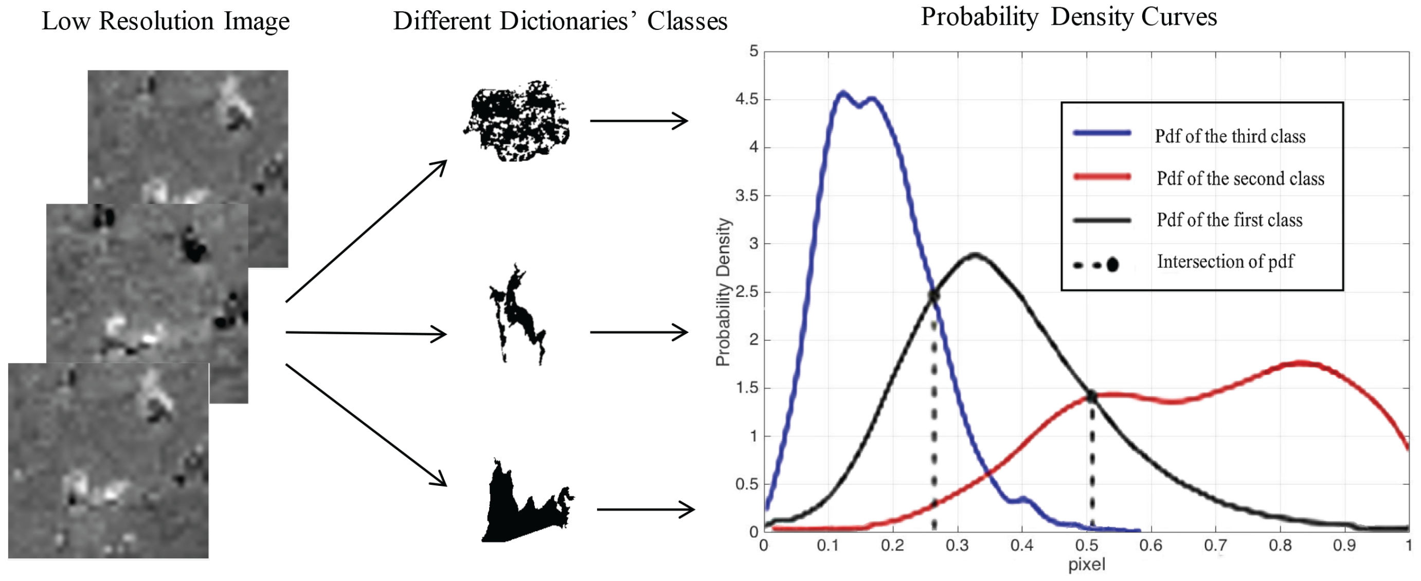
3.3. Classification of Test Image
3.4. Reconstruction
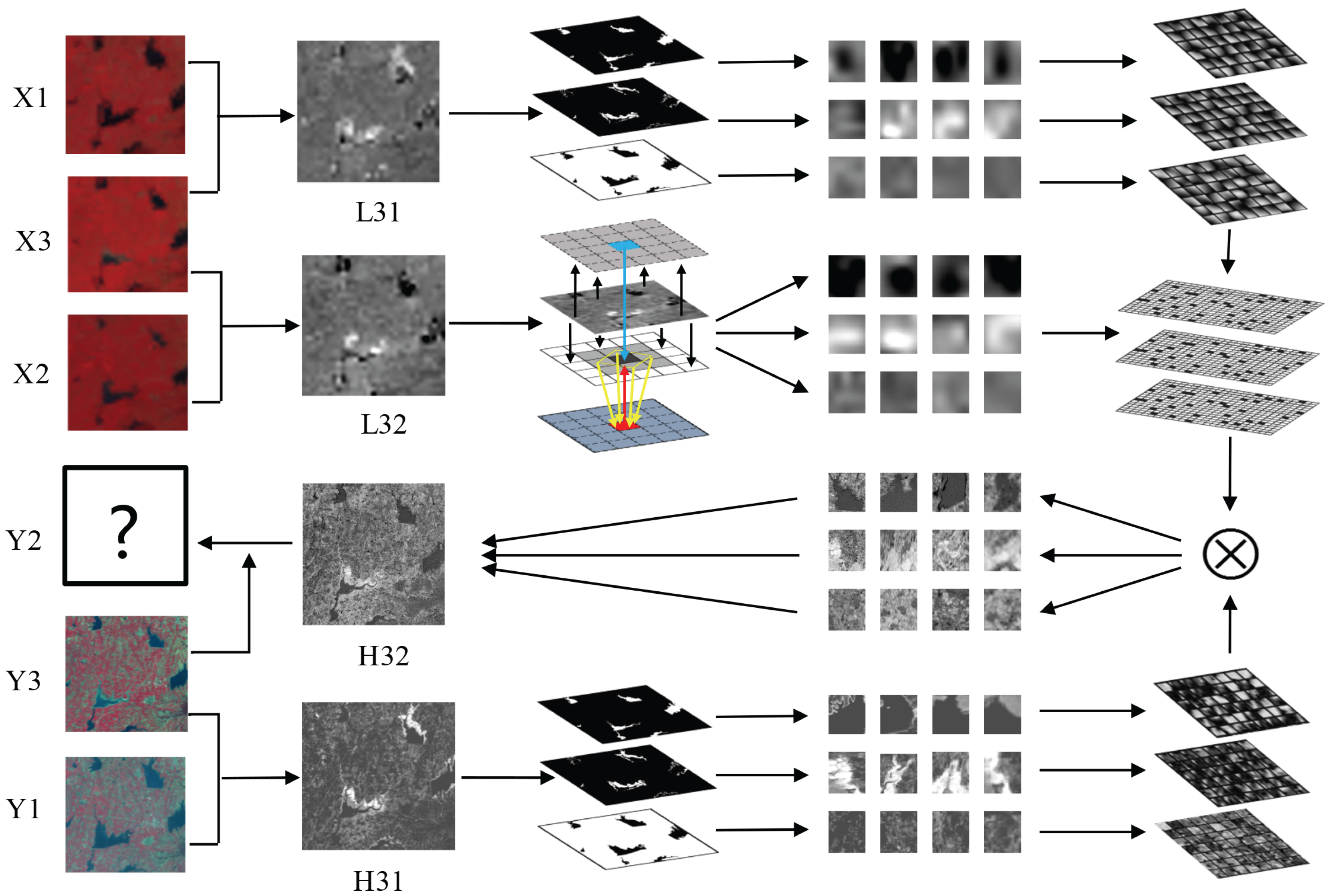
3.5. Diagram of MDBFM
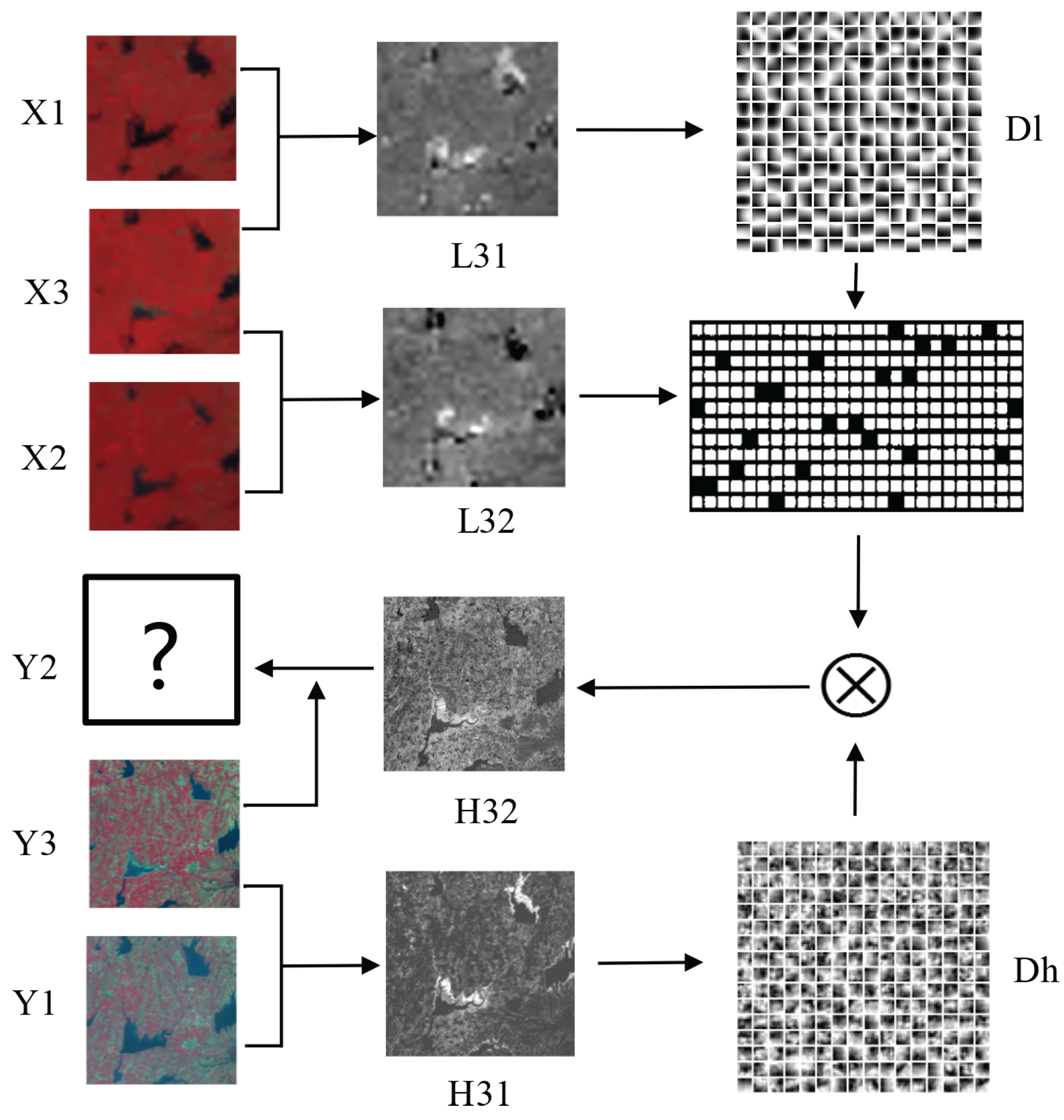
- The MODIS image is scaled up to the size of Landsat and the difference image is obtained after preprocessing.
- is classified manually into classes (e.g., three classes, namely, lake, degradation area of lake, and forest in the type changes dataset). For each class, patches are extracted from the difference images and are stacked into training sample matrixes.
- For every class, the high- and low-resolution sample matrixes are combined to train dictionary pairs. The training process of the dictionary is the same as that of SPSTFM by using the K-SVD method.
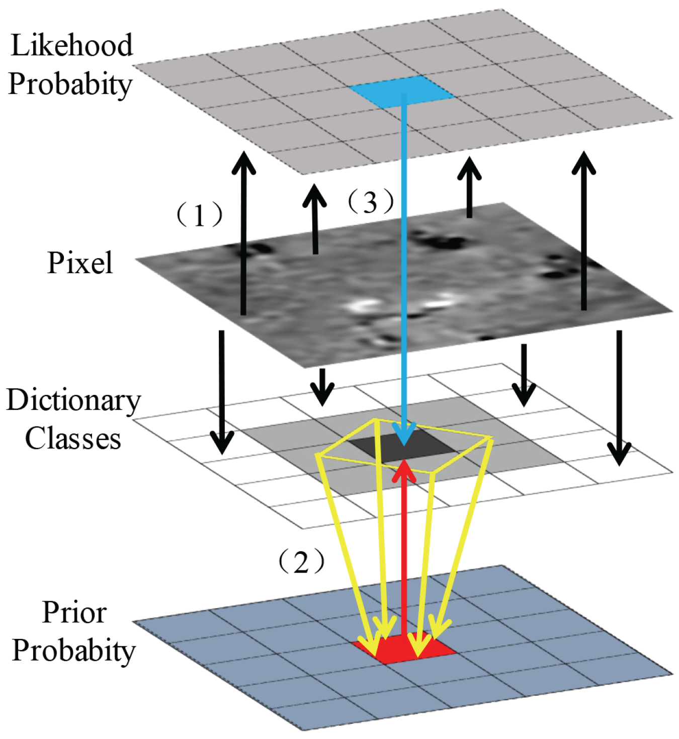
- After preprocessing, and are differentiated to obtain the difference image . Bayesian is then applied to classify the input difference image pixel-by-pixel.
- is divided into patches according to the classification result. The patches with the same label are stacked to form input matrixes of this class.
- For each input matrix, the sparse representation coefficients are obtained with the corresponding low-resolution dictionary by using OMP.
- The sparse representation coefficients of each class are multiplied by the high-resolution dictionaries to obtain the high-resolution matrix.
- The high-resolution matrix is reshaped, and the high-resolution patches are obtained.
- Each high-resolution patch is placed in its proper location and is averaged in the overlap regions. The Landsat-like difference image is then obtained.
- Using another difference image as input, the other Landsat-like difference image can be reconstructed in the same way.
- Equation (4) is applied to fuse and as well as to obtain the final reconstruction Landsat-like image.
4. Experiment
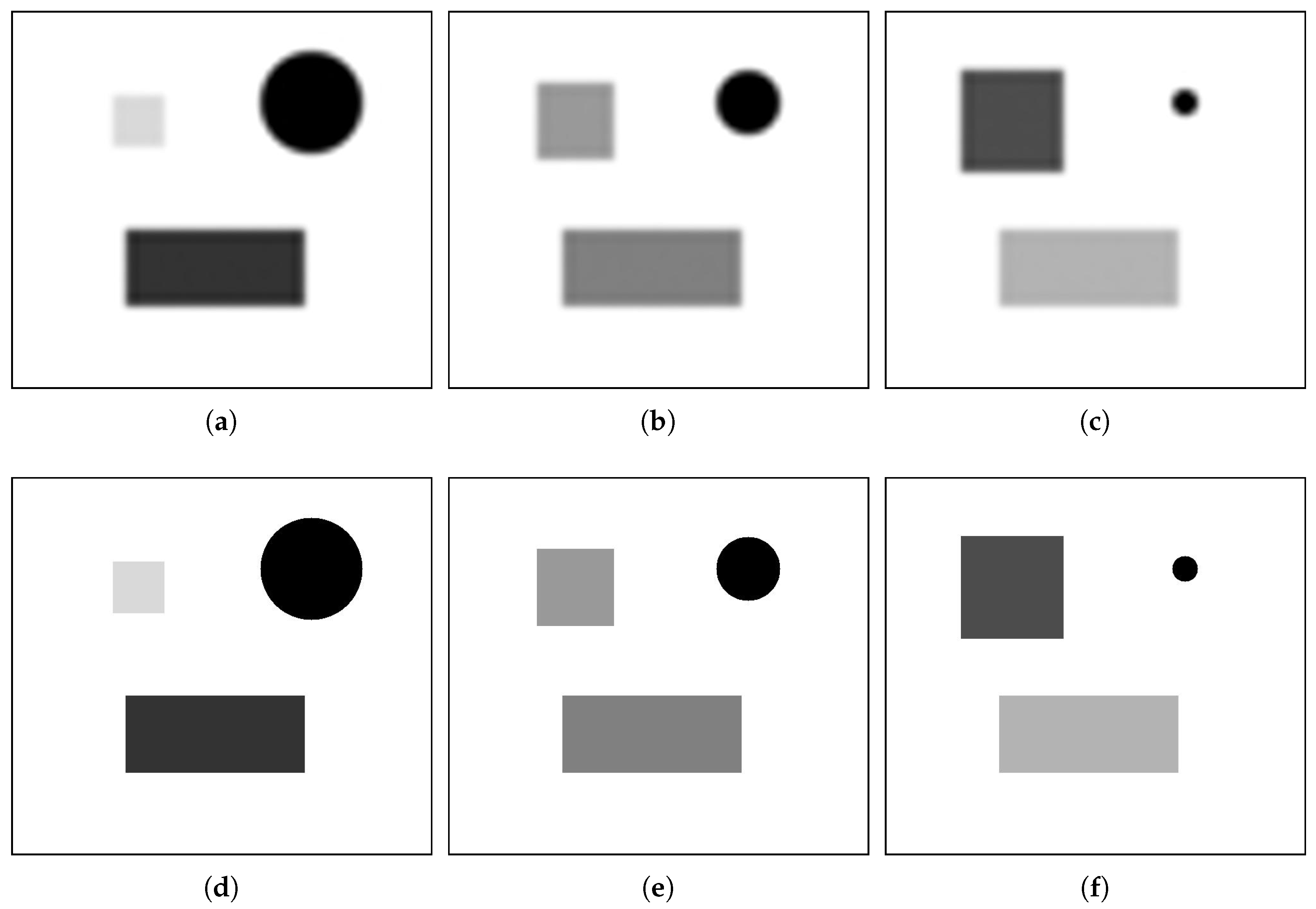
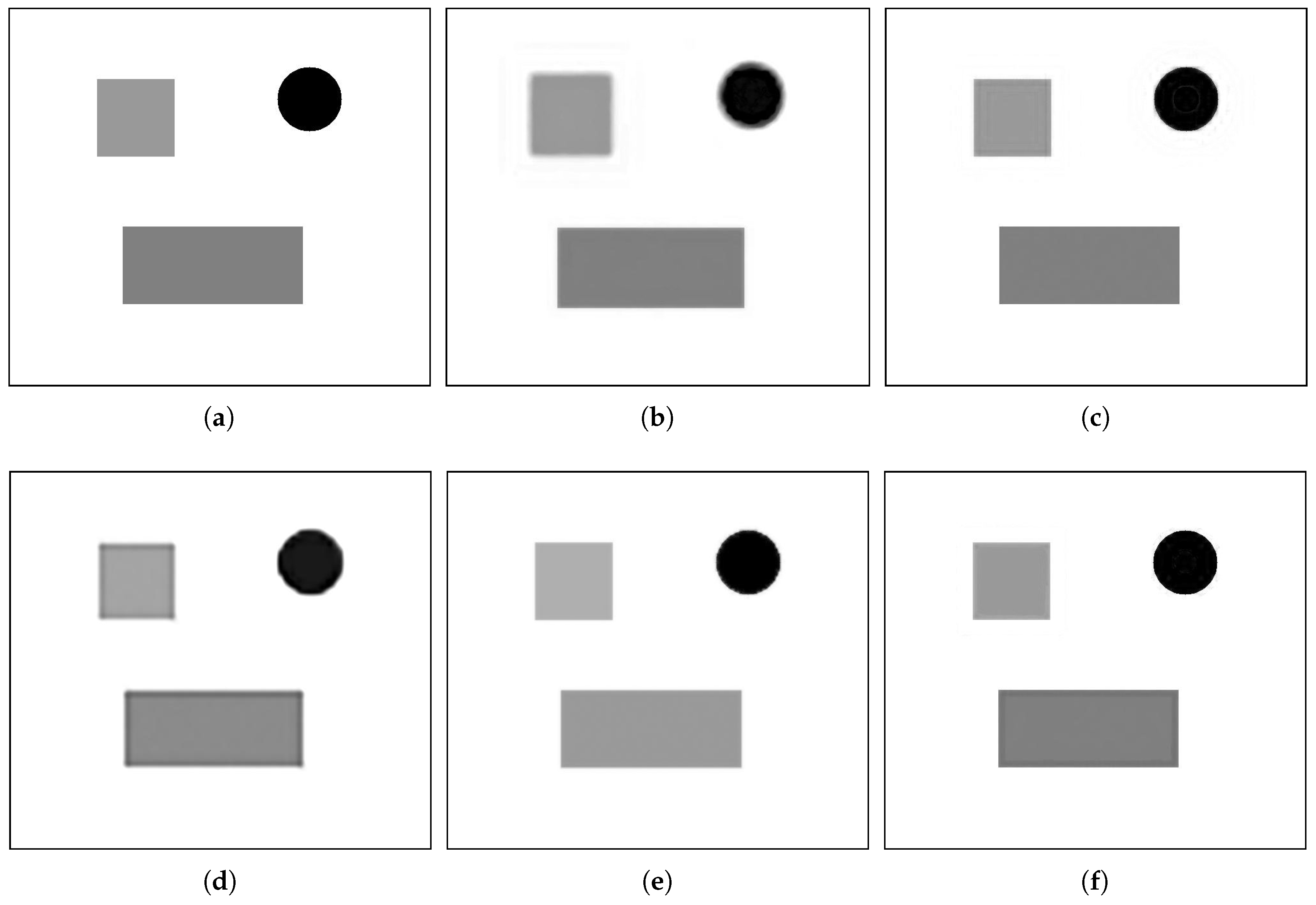
4.1. Simulated Data
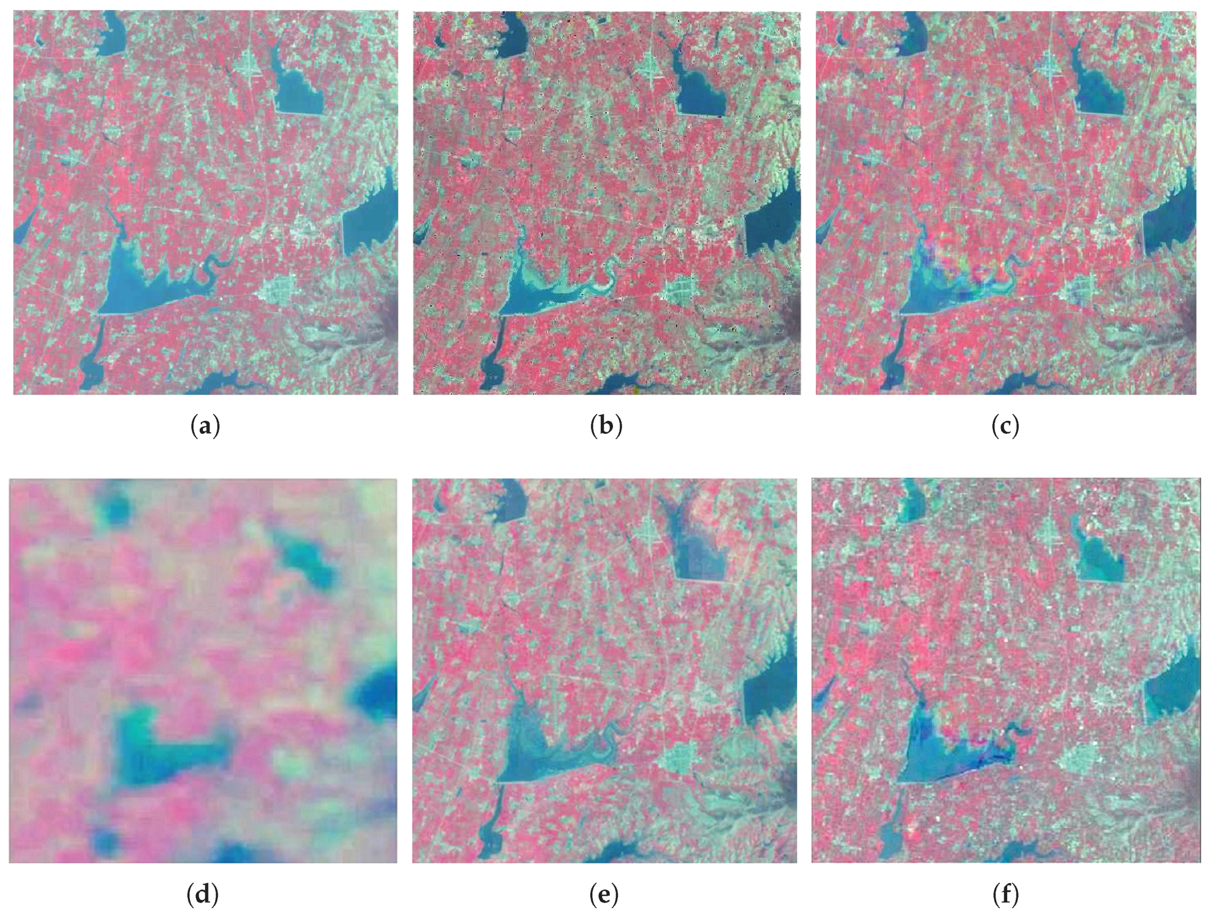
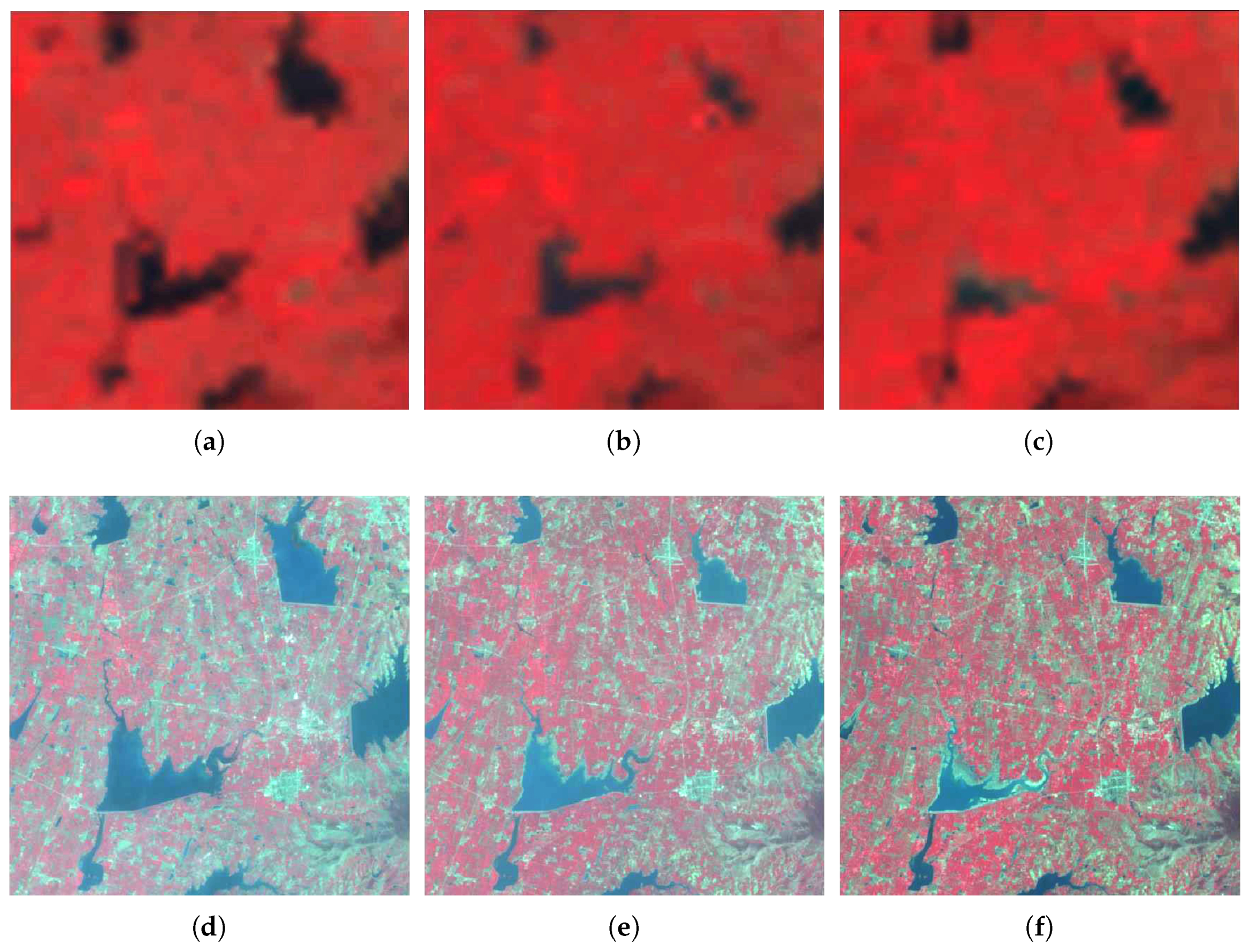
4.2. Remote Sensing Images with Type Changes
Data Sources
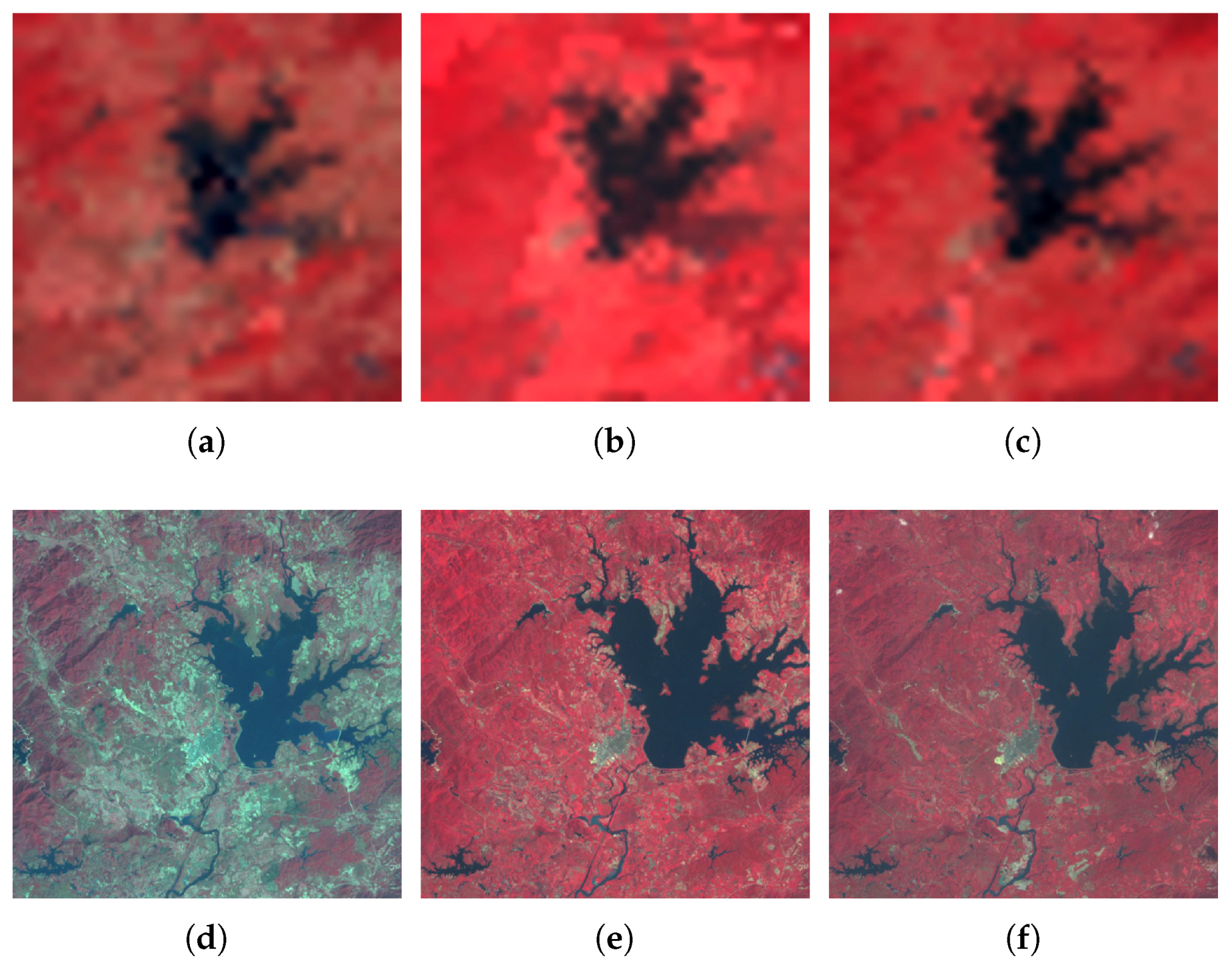
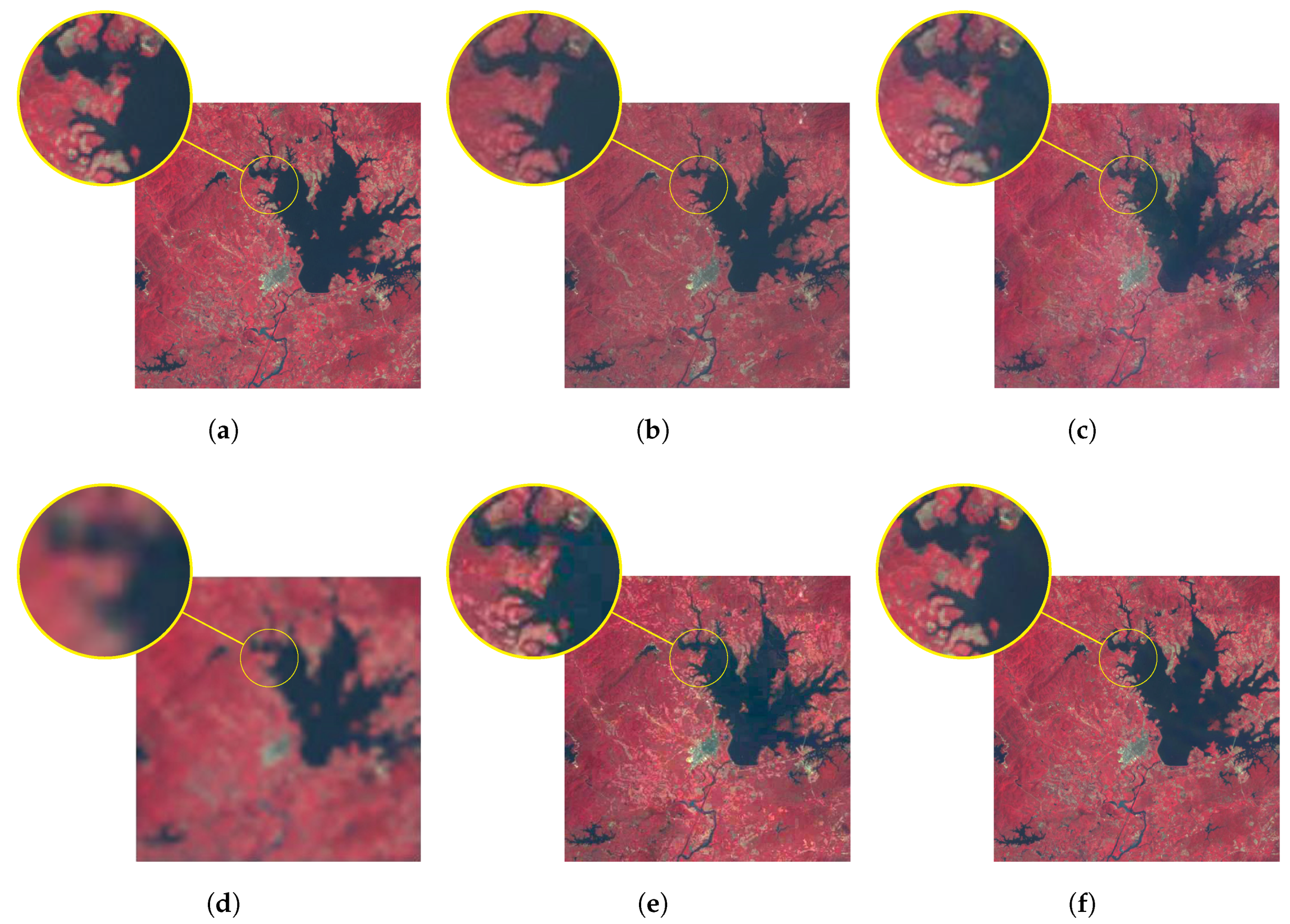
4.3. Remote Sensing Images with Phenology Changes
5. Discussion
6. Conclusions
Acknowledgments
Author Contributions
Conflicts of Interest
Abbreviations
| MODIS | Moderate resolution Imaging Spectroradiometer |
| CNN | Convolutional Neural Network |
| OMP | Orthogonal Matching Pursuit |
| MAP | Maximum A Posterior |
| SLC | Scan Line Corrector |
References
- Arvor, D.; Jonathan, M.; Meirelles, M.S.P.; Dubreuil, V.; Durieux, L. Classification of MODIS EVI time series for crop mapping in the state of Mato Grosso, Brazil. Int. J. Remote Sens. 2011, 32, 7847–7871. [Google Scholar] [CrossRef]
- Notarnicola, C.; Duguay, M.; Moelg, N.; Schellenberger, T.; Tetzlaff, A.; Monsorno, R.; Costa, A.; Steurer, C.; Zebisch, M. Snow cover maps from MODIS images at 250 m resolution, Part 1: Algorithm description. Remote Sens. 2013, 5, 110–126. [Google Scholar] [CrossRef]
- Shabanov, N.; Wang, Y.; Buermann, W.; Dong, J.; Hoffman, S.; Smith, G.; Tian, Y.; Knyazikhin, Y.; Myneni, R. Effect of foliage spatial heterogeneity in the MODIS LAI and FPAR algorithm over broadleaf forests. Remote Sens. Environ. 2003, 85, 410–423. [Google Scholar] [CrossRef]
- Swathika, R.; Sharmila, T.S. Multi-resolution spatial incorporation for MODIS and LANDSAT image fusion using CSSTARFM. In Proceedings of the 2016 IEEE Region 10 Conference (TENCON), Marina Bay Sands, Singapore, 22–25 November 2016; pp. 691–696. [Google Scholar]
- González-Sanpedro, M.; Le Toan, T.; Moreno, J.; Kergoat, L.; Rubio, E. Seasonal variations of leaf area index of agricultural fields retrieved from Landsat data. Remote Sens. Environ. 2008, 112, 810–824. [Google Scholar] [CrossRef]
- Zhang, Y. Understanding image fusion. Photogramm. Eng. Remote Sens. 2004, 70, 657–661. [Google Scholar]
- Hilker, T.; Wulder, M.A.; Coops, N.C.; Seitz, N.; White, J.C.; Gao, F.; Masek, J.G.; Stenhouse, G. Generation of dense time series synthetic Landsat data through data blending with MODIS using a spatial and temporal adaptive reflectance fusion model. Remote Sens. Environ. 2009, 113, 1988–1999. [Google Scholar] [CrossRef]
- Huang, B.; Wang, J.; Song, H.; Fu, D.; Wong, K. Generating high spatiotemporal resolution land surface temperature for urban heat island monitoring. IEEE Geosci. Remote Sens. Lett. 2013, 10, 1011–1015. [Google Scholar] [CrossRef]
- Walker, J.; De Beurs, K.; Wynne, R.; Gao, F. Evaluation of Landsat and MODIS data fusion products for analysis of dryland forest phenology. Remote Sens. Environ. 2012, 117, 381–393. [Google Scholar] [CrossRef]
- Weng, Q.; Fu, P.; Gao, F. Generating daily land surface temperature at Landsat resolution by fusing Landsat and MODIS data. Remote Sens. Environ. 2014, 145, 55–67. [Google Scholar] [CrossRef]
- Cammalleri, C.; Anderson, M.; Gao, F.; Hain, C.; Kustas, W. A data fusion approach for mapping daily evapotranspiration at field scale. Water Resour. Res. 2013, 49, 4672–4686. [Google Scholar] [CrossRef]
- Gao, F.; Masek, J.; Schwaller, M.; Hall, F. On the blending of the Landsat and MODIS surface reflectance: Predicting daily Landsat surface reflectance. IEEE Trans. Geosci. Remote Sens. 2006, 44, 2207–2218. [Google Scholar]
- Hilker, T.; Wulder, M.A.; Coops, N.C.; Linke, J.; McDermid, G.; Masek, J.G.; Gao, F.; White, J.C. A new data fusion model for high spatial-and temporal-resolution mapping of forest disturbance based on Landsat and MODIS. Remote Sens. Environ. 2009, 113, 1613–1627. [Google Scholar] [CrossRef]
- Zhu, X.; Chen, J.; Gao, F.; Chen, X.; Masek, J.G. An enhanced spatial and temporal adaptive reflectance fusion model for complex heterogeneous regions. Remote Sens. Environ. 2010, 114, 2610–2623. [Google Scholar] [CrossRef]
- Michishita, R.; Chen, L.; Chen, J.; Zhu, X.; Xu, B. Spatiotemporal reflectance blending in a wetland environment. Int. J. Digit. Earth 2015, 8, 364–382. [Google Scholar] [CrossRef]
- Yang, J.; Wright, J.; Huang, T.S.; Ma, Y. Image super-resolution via sparse representation. IEEE Trans. Image Process. 2010, 19, 2861–2873. [Google Scholar] [CrossRef] [PubMed]
- Huang, B.; Song, H. Spatiotemporal reflectance fusion via sparse representation. IEEE Trans. Geosci. Remote Sens. 2012, 50, 3707–3716. [Google Scholar] [CrossRef]
- Dong, C.; Loy, C.C.; He, K.; Tang, X. Learning a deep convolutional network for image super-resolution. In European Conference on Computer Vision; Springer: Cham, Switzerland, 2014; pp. 184–199. [Google Scholar]
- Zhu, X.; Helmer, E.H.; Gao, F.; Liu, D.; Chen, J.; Lefsky, M.A. A flexible spatiotemporal method for fusing satellite images with different resolutions. Remote Sens. Environ. 2016, 172, 165–177. [Google Scholar] [CrossRef]
- Aharon, M.; Elad, M.; Bruckstein, A. rmk-SVD: An algorithm for designing overcomplete dictionaries for sparse representation. IEEE Trans. Signal Process. 2006, 54, 4311–4322. [Google Scholar] [CrossRef]
- Chen, S.S.; Donoho, D.L.; Saunders, M.A. Atomic decomposition by basis pursuit. SIAM Rev. 2001, 43, 129–159. [Google Scholar] [CrossRef]
- Gorodnitsky, I.F.; Rao, B.D. Sparse signal reconstruction from limited data using FOCUSS: A re-weighted minimum norm algorithm. IEEE Trans. Signal Process. 1997, 45, 600–616. [Google Scholar] [CrossRef]
- Pati, Y.C.; Rezaiifar, R.; Krishnaprasad, P. Orthogonal matching pursuit: Recursive function approximation with applications to wavelet decomposition. In Proceedings of the 1993 Conference Record of the Twenty-Seventh Asilomar Conference on Signals, Systems and Computers, Pacific Grove, CA, USA, 1–3 November 1993; pp. 40–44. [Google Scholar]
- He, C.; Shi, P.; Xie, D.; Zhao, Y. Improving the normalized difference built-up index to map urban built-up areas using a semiautomatic segmentation approach. Remote Sens. Lett. 2010, 1, 213–221. [Google Scholar] [CrossRef]
- Wu, F.Y. The potts model. Rev. Mod. Phys. 1982, 54, 235. [Google Scholar] [CrossRef]
- Boykov, Y.; Kolmogorov, V. An experimental comparison of min-cut/max-flow algorithms for energy minimization in vision. IEEE Trans. Pattern Anal. Mach. Intell. 2004, 26, 1124–1137. [Google Scholar] [CrossRef] [PubMed]


| Require: sample matrix Z, dictionary dimension S, iterations J | ||
| Initialization: initialize dictionary D by randomly selecting S columns in sample matrix Z | ||
| 1. | Apply OMP to compute sparse coefficients. | |
| 2. | Update each column s in dictionary, and stop until convergence: | |
| (1) | Multiply row s in the sparse matrix with column s in the dictionary to obtain | |
| (2) | Compute the overall representation error matrix | |
| (3) | Restrict by the remaining columns corresponding to column s in dictionary, and then obtain | |
| (4) | Apply to , | |
| (5) | Replace column k in the dictionary with the first column of U, and then update by | |
| (6) | Increase iterations J | |
| Index | STARFM | SPSTFM | SRCNN | FSDAF | MDBFM |
|---|---|---|---|---|---|
| RMSE | 0.0068 | 0.0041 | 0.0052 | 0.0042 | 0.0035 |
| AAD | 0.0047 | 0.0013 | 0.0035 | 0.0016 | 0.0013 |
| R | 0.8234 | 0.9856 | 0.8827 | 0.9731 | 0.9894 |
| SSIM | 0.8349 | 0.8866 | 0.8195 | 0.8664 | 0.9151 |
| Index | Channel | STARFM | SPSTFM | SRCNN | FSDAF | MDBFM |
|---|---|---|---|---|---|---|
| RMSE | Red | 0.0072 | 0.0033 | 0.0151 | 0.0041 | 0.0032 |
| Green | 0.0102 | 0.0055 | 0.0147 | 0.0031 | 0.0046 | |
| NIR | 0.0103 | 0.0068 | 0.0152 | 0.0074 | 0.0047 | |
| AAD | Red | 0.0041 | 0.0026 | 0.0149 | 0.0028 | 0.0027 |
| Green | 0.0066 | 0.0042 | 0.0142 | 0.0021 | 0.0033 | |
| NIR | 0.0074 | 0.0052 | 0.0146 | 0.0054 | 0.0034 | |
| R | Red | 0.7834 | 0.8946 | 0.7346 | 0.8444 | 0.9169 |
| Green | 0.7225 | 0.8998 | 0.7076 | 0.8215 | 0.9321 | |
| NIR | 0.7555 | 0.9421 | 0.6888 | 0.9090 | 0.9479 | |
| SSIM | Red | 0.7329 | 0.7803 | 0.7162 | 0.7521 | 0.8506 |
| Green | 0.7058 | 0.7780 | 0.6983 | 0.7363 | 0.8626 | |
| NIR | 0.7175 | 0.7562 | 0.6528 | 0.7235 | 0.7954 |
| Index | Channel | STARFM | SPSTFM | SRCNN | FSDAF | MDBFM |
|---|---|---|---|---|---|---|
| RMSE | Red | 0.0062 | 0.0045 | 0.0220 | 0.0046 | 0.0039 |
| Green | 0.0059 | 0.0048 | 0.0196 | 0.0043 | 0.0042 | |
| NIR | 0.0121 | 0.0051 | 0.0281 | 0.0074 | 0.0046 | |
| AAD | Red | 0.0034 | 0.0022 | 0.0188 | 0.0022 | 0.0015 |
| Green | 0.0032 | 0.0041 | 0.0124 | 0.0020 | 0.0017 | |
| NIR | 0.0043 | 0.0040 | 0.0236 | 0.0041 | 0.0027 | |
| R | Red | 0.8842 | 0.9147 | 0.8254 | 0.9103 | 0.9297 |
| Green | 0.9128 | 0.8976 | 0.8328 | 0.8983 | 0.8932 | |
| NIR | 0.8614 | 0.8955 | 0.8132 | 0.8808 | 0.9691 | |
| SSIM | Red | 0.7978 | 0.8667 | 0.7410 | 0.8574 | 0.8947 |
| Green | 0.8314 | 0.8850 | 0.7409 | 0.8517 | 0.8798 | |
| NIR | 0.7570 | 0.8806 | 0.7417 | 0.8406 | 0.8904 |
© 2017 by the authors. Licensee MDPI, Basel, Switzerland. This article is an open access article distributed under the terms and conditions of the Creative Commons Attribution (CC BY) license (http://creativecommons.org/licenses/by/4.0/).
Share and Cite
He, C.; Zhang, Z.; Xiong, D.; Du, J.; Liao, M. Spatio-Temporal Series Remote Sensing Image Prediction Based on Multi-Dictionary Bayesian Fusion. ISPRS Int. J. Geo-Inf. 2017, 6, 374. https://doi.org/10.3390/ijgi6110374
He C, Zhang Z, Xiong D, Du J, Liao M. Spatio-Temporal Series Remote Sensing Image Prediction Based on Multi-Dictionary Bayesian Fusion. ISPRS International Journal of Geo-Information. 2017; 6(11):374. https://doi.org/10.3390/ijgi6110374
Chicago/Turabian StyleHe, Chu, Zhi Zhang, Dehui Xiong, Juan Du, and Mingsheng Liao. 2017. "Spatio-Temporal Series Remote Sensing Image Prediction Based on Multi-Dictionary Bayesian Fusion" ISPRS International Journal of Geo-Information 6, no. 11: 374. https://doi.org/10.3390/ijgi6110374
APA StyleHe, C., Zhang, Z., Xiong, D., Du, J., & Liao, M. (2017). Spatio-Temporal Series Remote Sensing Image Prediction Based on Multi-Dictionary Bayesian Fusion. ISPRS International Journal of Geo-Information, 6(11), 374. https://doi.org/10.3390/ijgi6110374