Forest above Ground Biomass Inversion by Fusing GLAS with Optical Remote Sensing Data

Abstract

Forest biomass is an important parameter for quantifying and understanding biological and physical processes on the Earth’s surface. Rapid, reliable, and objective estimations of forest biomass are essential to terrestrial ecosystem research. The Geoscience Laser Altimeter System (GLAS) produced substantial scientific data for detecting the vegetation structure at the footprint level. This study combined GLAS data with MODIS/BRDF (Bidirectional Reflectance Distribution Function) and ASTER GDEM data to estimate forest aboveground biomass (AGB) in Xishuangbanna, Yunnan Province, China. The GLAS waveform characteristic parameters were extracted using the wavelet method. The ASTER DEM was used to compute the terrain index for reducing the topographic influence on the GLAS canopy height estimation. A neural network method was applied to assimilate the MODIS BRDF data with the canopy heights for estimating continuous forest heights. Forest leaf area indices (LAIs) were derived from Landsat TM imagery. A series of biomass estimation models were developed and validated using regression analyses between field-estimated biomass, canopy height, and LAI. The GLAS-derived canopy heights in Xishuangbanna correlated well with the field-estimated AGB (R² = 0.61, RMSE = 52.79 Mg/ha). Combining the GLAS estimated canopy heights and LAI yielded a stronger correlation with the field-estimated AGB (R² = 0.73, RMSE = 38.20 Mg/ha), which indicates that the accuracy of the estimated biomass in complex terrains can be improved significantly by integrating GLAS and optical remote sensing data.

1. Introduction

As a primary component of the terrestrial ecosystem, forests are the largest terrestrial carbon sink and the most economical carbon absorber [1]. However, spatial heterogeneity and uncertainty in carbon sink estimates typically are common in different forests and different regions [2,3,4]. Forest biomass, accounting for 90% of the terrestrial vegetation biomass on the earth [5], directly and quantitatively reflects the amount of carbon storage in a forest and is the most important index and vegetation structure parameter used to estimate forest ecosystem productivity and to study the carbon cycle process. Therefore, the rapid and reliable estimation of forest biomass and its spatial distribution is essential to the studies of regional and global carbon cycle and climate change.

Forest biomass is the total dry weight of organic matter in the forest community during a specified time period [5]. Traditional methods for measuring forest biomass, such as field surveys that are human- and cost-intensive, can only obtain measurements at some scales and may lead to destructive effects on the ecosystem. Remote sensing provides an alternative approach to monitor and measure forest biomass more efficiently. Optical remote sensing, the most commonly used approach, has certain advantages in obtaining forest stand level structure parameters for forest biomass estimation, but these parameters are subject to various kinds of error and many restrictions [6], including the vegetation index (e.g., NDVI) saturation, atmospheric correction, and cloudy and rainy weathers. The development of microwave remote sensing has produced more reliable data for measuring biomass under all weather conditions, but the signal saturation problem may still exist [7]. Although polarimetric interferometry SAR/InSAR can address the loss of the estimation accuracy caused by forest density and structure change, it has restricted data application in regional or global forest structure parameter inversion due to costly data acquisition and other factors [8].

LiDAR (Light Detection and Ranging) has been used extensively to estimate vegetation canopy height, forest stock, and aboveground biomass (AGB). The accuracy of LiDAR-measured vegetation height and biomass typically is 5–10 times greater than that from optical remote sensing data [9,10,11]. Sun et al. [12,13] conducted theoretical simulations of the Geoscience Laser Altimeter System (GLAS) waveform and forest structure parameter inversion. According to their results, GLAS data can be used to estimate forest stand height. Pang et al. [14] used airborne LiDAR data to extract the average tree height in the Mountain Zulai Forest Trial Plot, Tai’an City, Shandong Province, China, with an overall accuracy of up to 90.59%. Means et al. [15] used airborne LiDAR to study the vegetation heights of an Oregon forest stand in the Western United States and determined that the relationship between forest heights and AGB was significant up to 1300 Mg/ha, even in very dense forests. Since the GLAS points are discontinuous with relatively low spatial density, they should be combined with other continuous remotely-sensed data to obtain a continuous high-precision canopy height distribution and biomass estimation [16]. Therefore, to obtain forest biomass data at a regional scale, Nelson et al. [17] used GLAS and MODIS data to estimate the forest growing stock in Siberia. The results show that the combination of GLAS and optical data can significantly improve the accuracy of biomass derivation results. Lefsky et al. [18] estimated forest biomass by combining forest biomass extracted from airborne LiDAR data and stand age information extracted from Landsat TM imagery. Huang et al. [19] estimated forest AGB within GLAS footprints in combination with airborne LiDAR data, the MODIS vegetation conversion product (MOD44B) and the MERIS land cover product for continuous mapping of the Yunnan forest AGB, with a coefficient of determination of 0.52 and a root mean square error (RMSE) of 31 Mg/ha.

LiDAR has great application potential for forest AGB estimation. In contrast to the high costs and spatial limitations of airborne LiDAR, GLAS has a wide observation view and global coverage and thus has advantages for large-scale forest biomass estimation research. Studies have been conducted to estimate the forest biomass in Xishuangbanna, Yunnan, China [20,21,22,23], but most of these studies focused on two-dimensional biomass modeling using optical remote sensing or a single parameter inversion of vegetation height. Steep slopes can lead to a mixed GLAS waveform, which causes difficulty in decomposing the waveform. In this study, we focused on forest horizontal and vertical structure information, as well as the terrain slope effect. GLAS, MODIS BRDF (Bidirectional Reflectance Distribution Function) data and Landsat TM imagery were used to obtain continuous canopy height, forest type, and LAI. Field measured canopy height and LAI were used to construct a multivariable regression model to achieve accurate forest AGB estimates. The method proposed in this study serves as an example for other forest structure and AGB estimates in high terrain areas.

2. Study Area and Experimental Data

2.1. Study Area

To evaluate and compare different models for estimating forest AGB, a study in Xishuangbanna Forest, south of Yunnan province, China, was conducted. The study site covers approximately 20,000 km² and is dominated by tropical rainforest, seasonal rainforest, subtropical evergreen broad-leaved forest, coniferous forest, bamboo, shrub, and grass. Rubber plantations are rapidly expanding. The area of rubber plantations has increased to 205,000 ha during the past 30 years and comprises approximately 27.06% of the total forest. The second dominated trees are tropical rainforests [24]. In this study we classified the forests into two categories: rubber plantations, and tropical rainforests.

2.2. GLAS Data

A detailed introduction to GLAS can be found in Lefsky et al. [10] and Wang et al. [25]. The data used in this study were GLA01 and GLA14 products acquired in February, 2009. GLA01 (Class 1A) records the number of each footprint and full waveform information, and GLA14 (Class 2) contains pulse record number, longitude, latitude, and elevation. A total of 1938 GLAS footprints fell within the study area.

2.3. MODIS BRDF Data

MODIS is a sensor with 36 wave bands onboard the Terra and Aqua satellites. MODIS BRDF is a four-level product with a spatial resolution of 500 m (Ver. 5) and in HDF-EOS format. MODIS BRDF data reflect the anisotropy of each pixel better and have the ability to retrieve vegetation structure [26]. The main algorithm of the MODIS BRDF represents the volumetric scattering and geometric-optical scattering by the Ross-Thick kernel and Li-Sparse Reciprocal kernel, named RTLSR, shown in Equation (1):

$$R\left(\theta ,\vartheta ,\varphi ,\Lambda \right)=f_{iso}(\Lambda )+f_{vol}(\Lambda )K_{vol}\left(\theta ,\vartheta ,\varphi \right)+f_{geo}(\Lambda )K_{geo}\left(\theta ,\vartheta ,\varphi \right)$$

(1)

where f_iso, f_vol, and f_geo are weights of isotropic scattering, volumetric scattering, and geometric-optical scattering, respectively; K_geo and K_vol are trigonometric functions of view zenith θ, illumination zenith ϑ, and relative azimuth ϕ; these functions provide shapes for the surface-scattering and volume-scattering BRDFs; R (θ, ϑ, ϕ, Λ) is the bidirectional reflectance distribution function for the waveband Λ.

The sub-product of the MODIS BRDF/Albedo data, termed MCD43A1, provides the weighting parameters for the RTLSR model, i.e., the weight of isotropic scattering, the weight of geometrical-optical scattering, and the weight of volumetric scattering. To synchronize with the GLAS data, the MCD43A1 products in February 2009 were used in this study.

2.4. Landsat TM Data

Landsat TM data were obtained freely from the Institute of Remote Sensing and Digital Earth (RADI), Chinese Academy of Sciences (CAS). The data have been ortho-rectified with a spatial resolution of 30 m from which LAI was derived. We studied 11 vegetation indices from TM data: NDVI (normalized difference vegetation index), DVI (difference vegetation index), SRVI (simple ratio vegetation index), PVI (perpendicular vegetation index), SAVI (soil-adjusted vegetation index), ARVI (atmospherically resistant vegetation index), EVI (enhanced vegetation index), TVI (triangular vegetation index), MSAVI (modified SAVI), SARVI (soil-adjusted ARVI), and MCARI (modified chlorophyll absorption in reflectance index), and established the statistical regression model for these indices and field measured LAI. The model of MSAVI and LAI performed best, which is used to derive LAI in the study, as shown in Equation (2) [27]:

$$y=4.4212x-0.0385$$

(2)

where y is LAI, and x is MSAVI.

2.5. ASTER GDEM Data

The ASTER DEM (Digital Elevation Model) data were downloaded from NASA to correct the influence of topographic slope on GLAS waveform parameter. The data was in GeoTIFF format with a WGS84 coordinate system. The second version of the DEM data covering the study area was used, and the spatial resolution is 30 m.

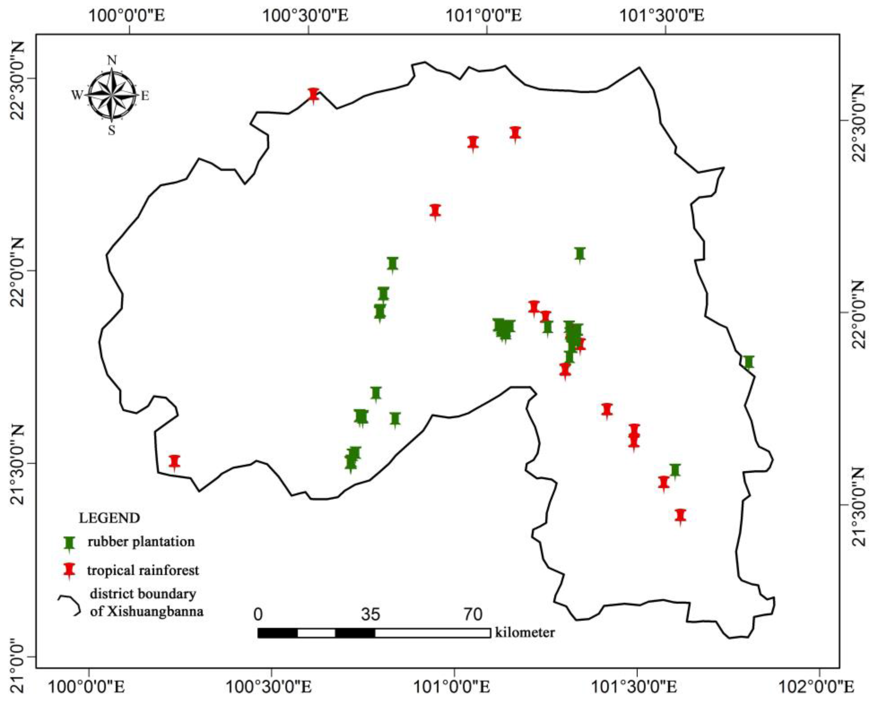
2.6. Ground Measured Data

Ground measurements were collected in January of 2012 and April of 2013 using a quadrat survey method and RTK-GPS, hand-held laser altimeter, measuring tape, diameter tape, angle gauge, and 3D TLS (Terrestrial Laser Scanner, Riegl VZ1000). Figure 1 shows the field sample GLAS footprints. The coordinate of each footprint was determined using the RTK-GPS. All trees with DBH exceeding 5 cm were measured within a circular area with a diameter of 30 m and centered on the center of each selected GLAS footprint. The geographic coordinates, dominant tree species, and terrain slope and slope aspect of each sample plot were recorded, and the DBH, and height of each sampled tree were measured. Some footprints were scanned with the TLS to acquire accurate vegetation heights for validating field-measured tree heights. Results showed that the errors in the field measurements were insignificant. The average height of all trees in one plot is used to represent the field-measured canopy height of this plot. Sixty-five plots for rubber plantations and 31 for tropical rainforests were sampled. A tropical seasonal rainforest biomass allometric equation is used to estimate the tropical rainforest [20]:

$$w=a\times D^b$$

(3)

where D is DBH, w is biomass, and a and b are parameters. However, when we applied this model to the study area, different factors, such as time change, terrain characteristics, and vegetation type, could bring errors. Therefore, a new parameter c was added to the biomass model developed in previous studies as follows:

$$w=a\times D^b+c$$

(4)

where c is a constant. Through a number of experiments, the c values for rubber plantation and tropical rainforest were found to be −8.99 and −32.12, respectively. We found that the modified models improved estimation accuracy of single tree (see Figure 2). The total biomass (Mg, dry weight) in each sample plot is the sum of all trees, and average biomass data (Mg/ha) is calculated. Subsequently, the biomass data were converted into a 500 m × 500 m grid corresponding to the spatial resolution of the MODIS data.

3. Methods

3.1. GLAS Data Processing

3.1.1. Pre-Processing

GLAS data preprocessing includes error elimination, data decompression, voltage conversion, and filtering. The IDL tool available on the National Snow and Ice Data Center (NSIDC) was used to read the binary GLAS data and convert them into ASCII text files. Data outliers caused by cloud and system noise were eliminated. To ensure that 544 samples completely comprise the vertical information within a footprint, the GLAS system records waveforms in the form of subsection compression, and the waveform data was decompressed based on the compression ratio. GLA01 and GLA14 were recorded as digital numbers in binary format. A list of ancillary products are required to produce GLAS standard products. ANC07 is one of GLAS ancillary products, which provides constants related to error, atmosphere, elevation and waveforms. We obtained the ANCO7 from the NSIDC. To get high-quality waveform data, a mean filtering method was applied to the GLAS waveform data in this study. Mean filtering is a common method for reducing the noise of waveform by averaging the waveform intensity within a local window [28].

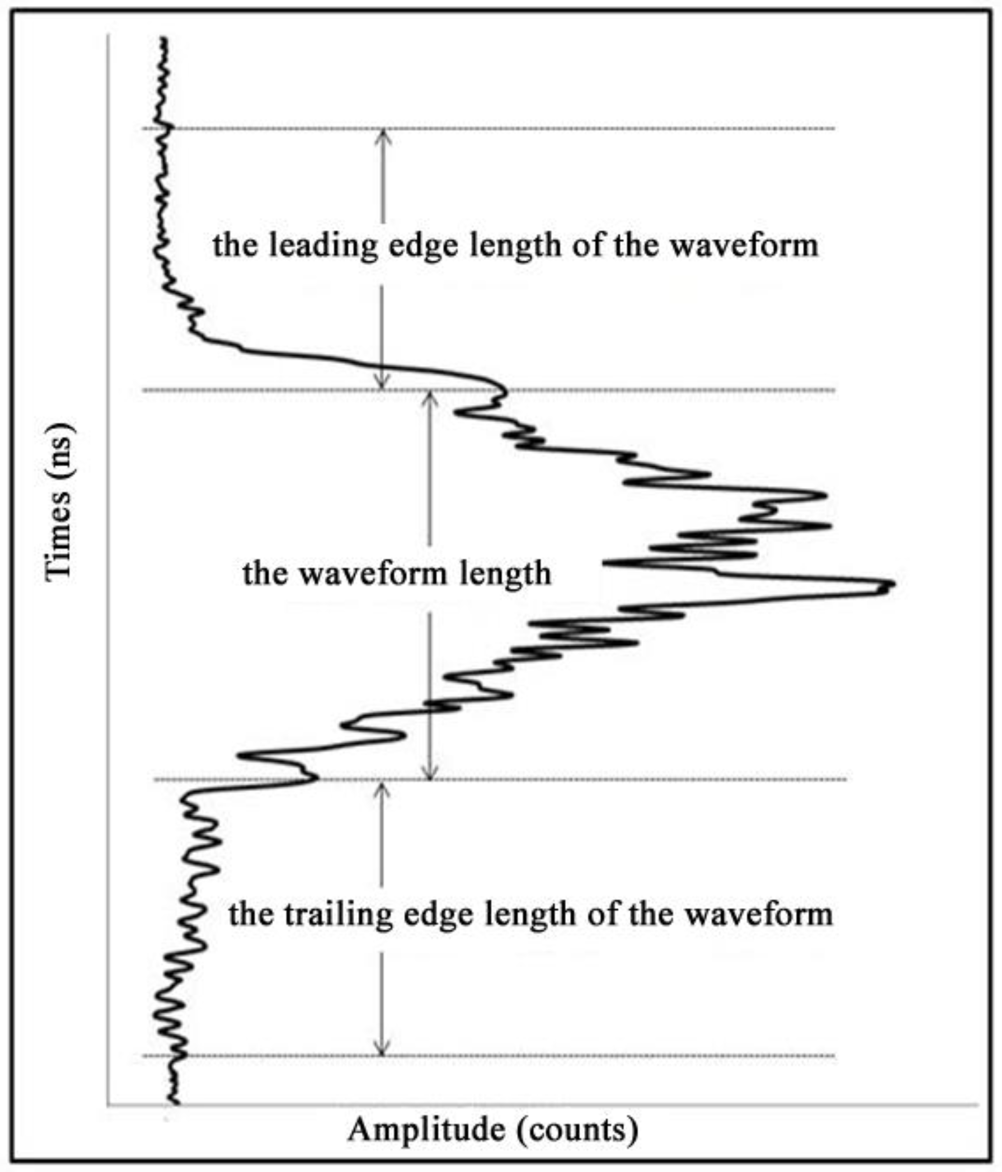
3.1.2. The GLAS Waveform Characteristics Extraction

The distance between the start of the signal and the last peak of a GLAS waveform is related to the height of the tallest tree in a footprint, although it cannot describe the height information of all trees within the footprint. Previous studies used the waveform length, leading edge, and trailing edge of the waveform to estimate the average canopy height [10,25], which can be expressed as the distance from the first peak of the waveform to the last peak (i.e., the peak of ground return) (Figure 3). We analyzed the echo data by building models to obtain the peak of the waveform position of different Gaussian waves. The wavelet analysis method is used to position the peak of the waveform and to extract waveform length information of the vegetation height peak [25]. Here, the front edge length of the waveform refers to the distance between the first Gaussian wave peak and the effective signal starting point. The front edge length reflects the total influence of the vegetation canopy roughness and the complex terrain relief on the echo signal. The distance between the last Gaussian peak at the trailing edge of the waveform and the ending point of the effective signal reflects the influence of topographic slope and surface relief on the echo signal.

3.1.3. Terrain Correction

The laser echo signal of a large footprint is the result of interaction between the laser pulse and the vegetation canopy and ground. Topographic slope has remarkable influence on the waveform, primarily explained by broadening and aliasing the waveform. This study builds a model based on the measured tree height (H), the waveform length (w), the leading edge length (l) and the trailing edge length (t) of the waveform, the topographic index (g) and the topographic standard deviation (s) to reduce the topographic slope influence [28].

The topographic index is a statistical parameter proposed by Lefsky et al. [10,11] to eliminate the influence of the terrain effect on full waveform data. The index is expressed as the difference between the maximum and minimum elevation values of an n × n window. The topographic standard deviation illustrates the feature of the topographic relief and reflects the terrain influence during the laser echo function process [11]. For the GLAS data and a DEM with a spatial resolution of 30 m, a 3 × 3 window can be used to reduce the terrain effect on the full waveform data. The topographic index and standard deviation can be calculated using a DEM. A total of 50 average canopy heights were used for modeling, as shown in

Table 1. Model fitting forest height lists.

No.	Parameters	Model	${\mathit{R}}^{\mathbf{2}}$
No. 1	$w$	$H=0.74w+2.56$	0.725
No. 2	$w,l$	$H=0.74w-0.04l+2.66$	0.726
No. 3	$w,g$	$H=0.74w-0.03g+3.29$	0.728
No. 4	$w,s$	$H=0.75w-0.10s+3.34$	0.729
No. 5	$w,l,t$	$H=0.76w+0.003l+0.33t+1.30$	0.750
No. 6	$w,l,g$	$H=0.75w-0.04l-0.03g+3.39$	0.729
No. 7	$w,l,s$	$H=0.75w-0.04l-0.1s+3.45$	0.730
No. 8	$w,l,t,g$	$H=0.77w+0.01l+0.35t-0.04g+2.24$	0.756
No. 9	$w,l,t,s$	$H=0.78w+0.005l+0.35t-0.13s+2.25$	0.757

.

In this study, we used the average of all trees heights within the footprint as the average canopy height of the footprint (H). From Table 1, we can see that the coefficient of determination of Model No. 9 is the best. A strong correlation exists between the waveform length and the vegetation height. The trailing length of the waveform can improve the correlation between the waveform length and the vegetation height well. Model No. 9 was used to correct the terrain for the GLAS waveform data.

3.2. MODIS Data Pre-Processing

A total of 10 bands of data from MODIS1-7 and three broad bands were provided in the MCD43A1 data, and each band has three BRDF parameters. The band index method proposed by Jiang et al. [29] was adopted to select the optimal band combination in selecting wave band. The red, blue, and near-infrared bands were selected. Through format conversion and a multiple-image mosaic, we obtained the BRDF image of the study area.

3.3. Fusion GLAS with MODIS to Estimate Tree Height

Due to the discontinuous distribution of the GLAS footprints, fusing GLAS with optical remote sensing data is an effective method to estimate large scale and continuous forest canopy heights. The model combining the MODIS BRDF data and GLAS was constructed by the BP neural network. The input layer contains nine nodes, including three BRDF parameters in the red, blue, and near-infrared bands. The output layer is the canopy height. The BP neural network was trained using 1938 GLAS points [28].

3.4. Biomass Modeling

First, canopy heights generated by fusing the GLAS data and MODIS/BRDF, and the measured biomass were used to build a univariate estimation model. Second, the above canopy heights, LAI, and measured biomass were used to build a multivariate biomass estimation model. Considering the coefficient of determination and F test value, we selected the optimal model and conducted a scale transformation and re-sampled the LAI at a resolution of 500 m instead of 30 m. Finally, the best forest AGB estimation model was developed for Xishuangbanna and was validated using an additional 21 field measured data.

4. Result Analysis

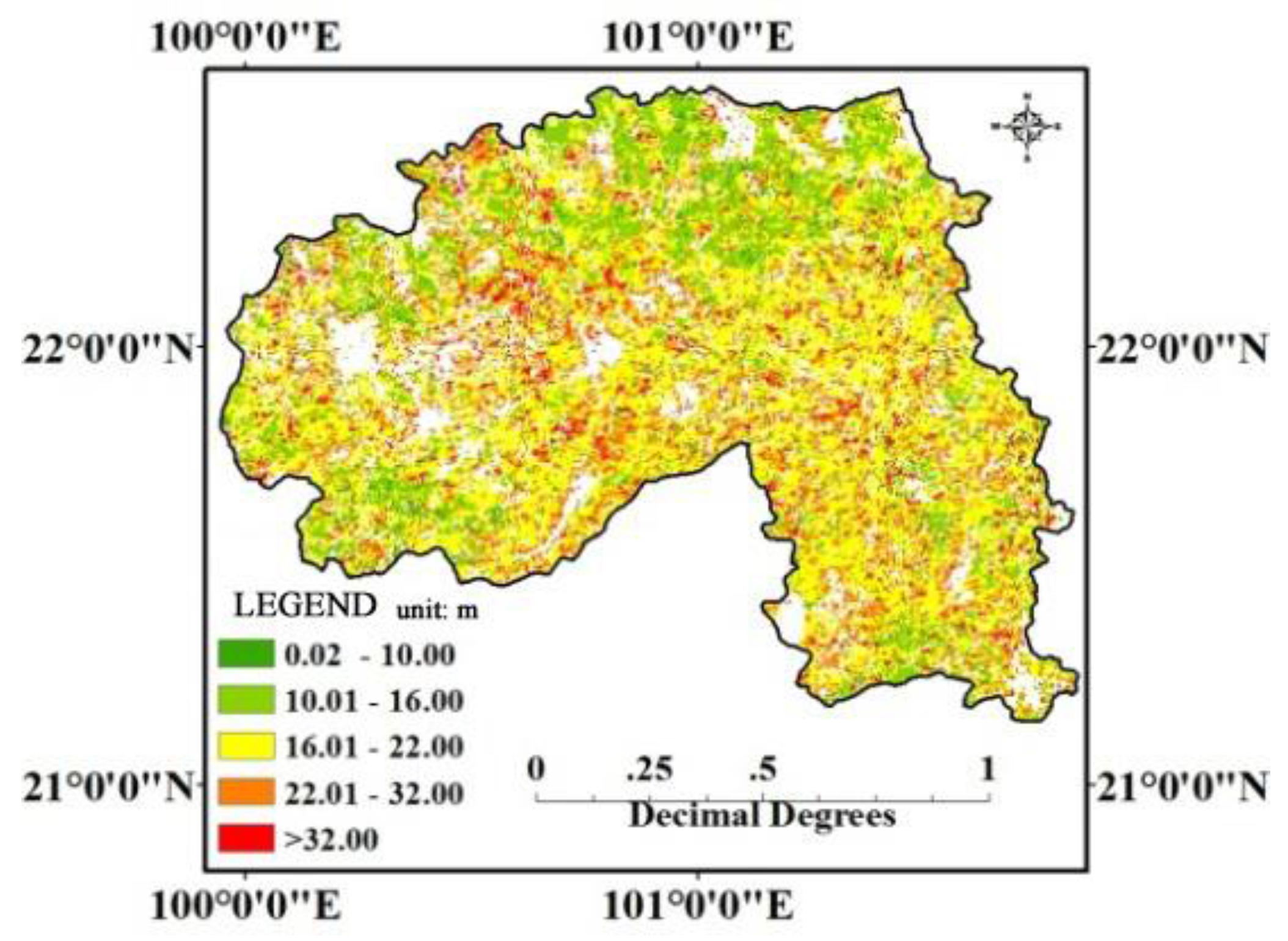
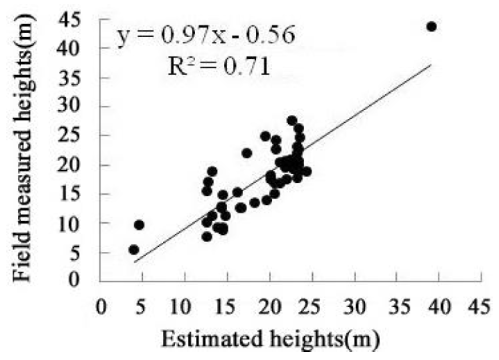
4.1. Continuous Vegetation Heights

Using GLAS sample plots and the MODIS BRDF image, we built a neural network model and obtained continuous vegetation heights in the study area, as shown in Figure 4. Forty-six field plots of tree heights were used for validating the estimated results, as shown in Figure 5. The results show that the coefficient of determination is approximately 0.71 (RMSE = 3.95 m) and that the method developed in this study can be used to estimate continuous vegetation heights.

Figure 5 shows that most vegetation heights ranged from 12 m to 25 m. The height of the tropical rainforest in Xishuangbanna was predominantly above 30 m. Broad leaf forest (height <30 m) is the major vegetation type and accounts for approximately 30.0% of the total area [30]. This indicates that our results are reasonable to some extent.

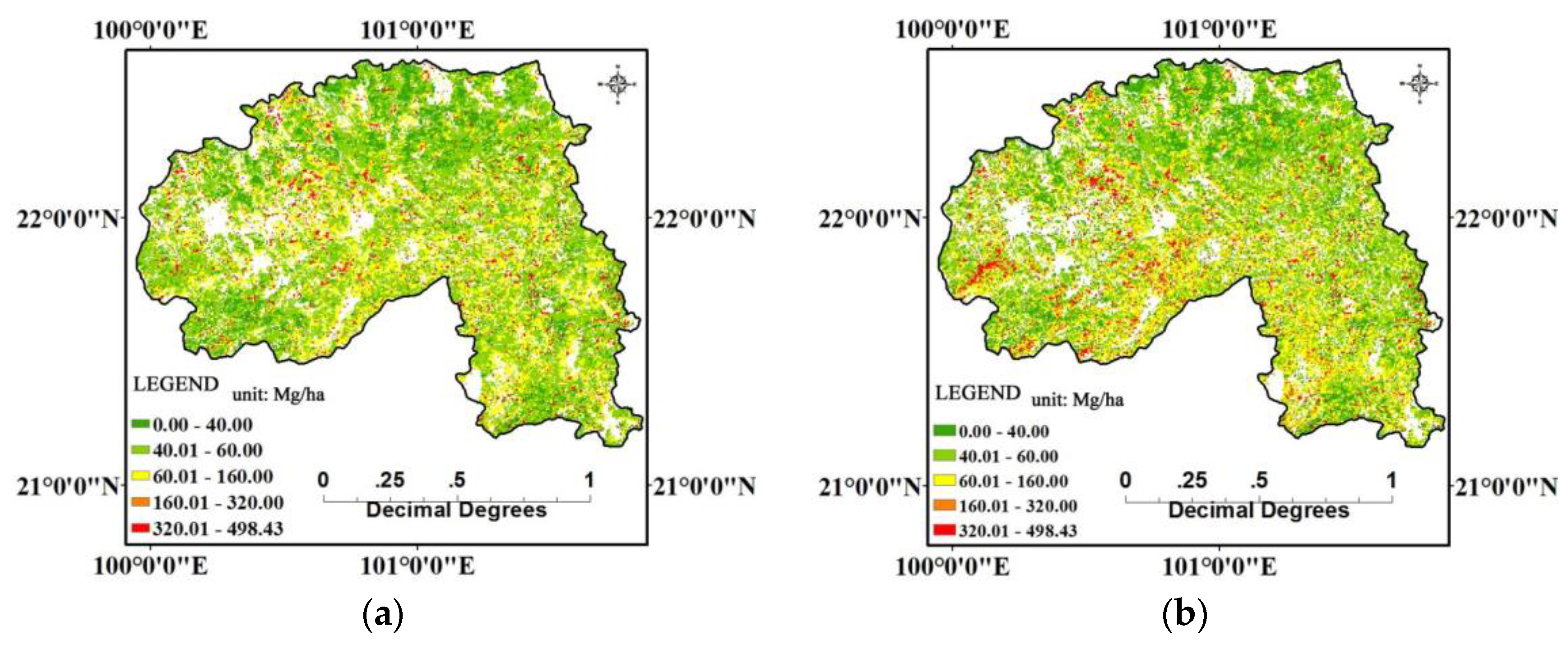
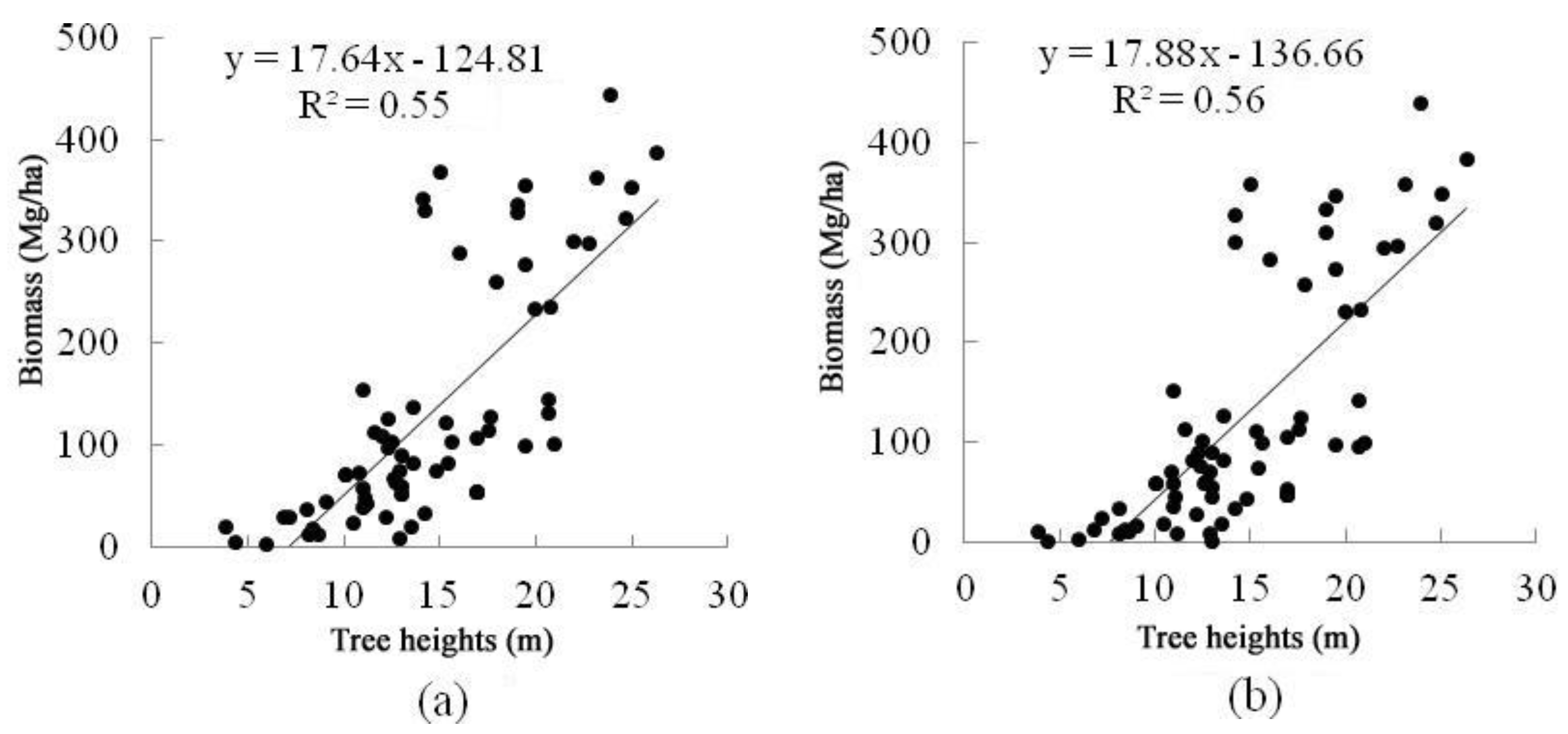
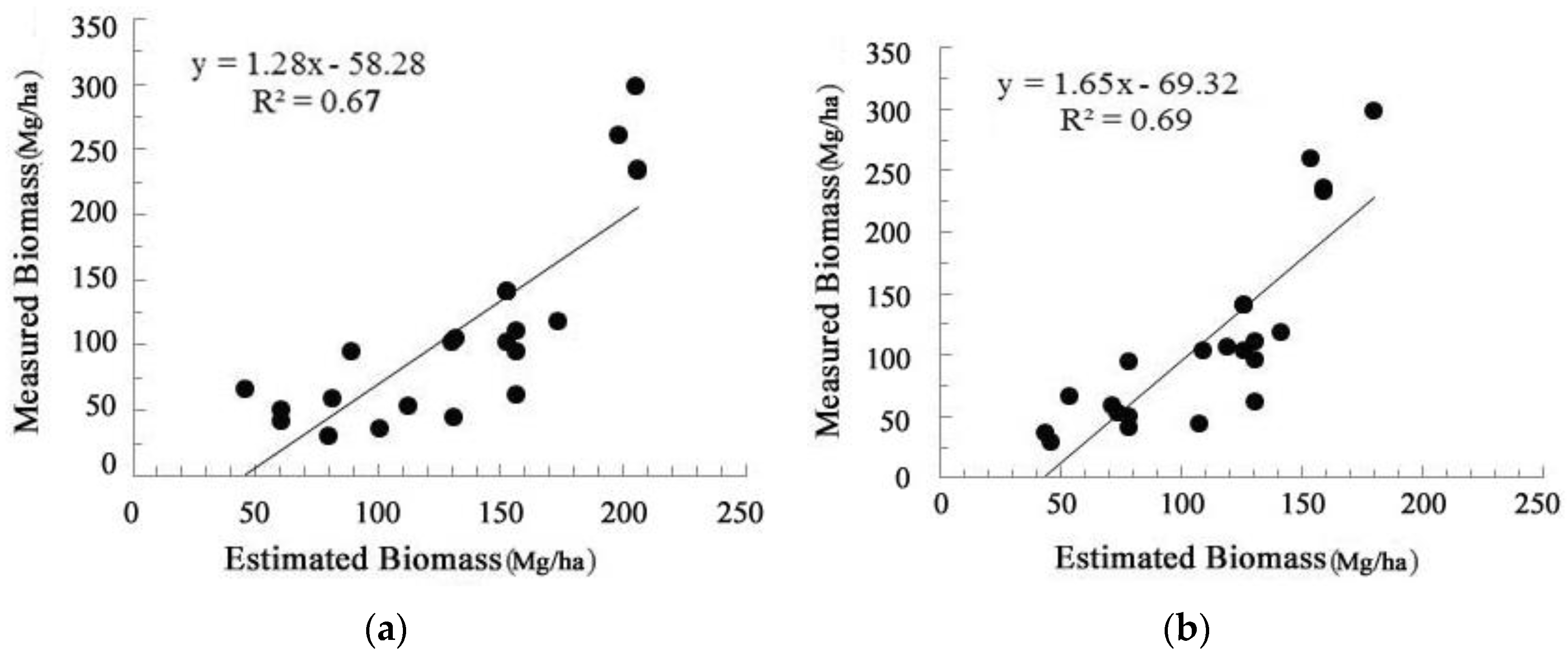
4.2. Forest AGB Estimation Results

A total of 75 field measured biomass data were used to build a series of regression models with continuous forest canopy height. The results listed in

Table 2. Regression models lists (Y represents the biomass. x₁ represents canopy height and x₂ represents LAI.).

Parameters	Function	No.	Models	R2	F Test
Height vs. Biomass	Polynomial Power function	No. 1	$y=1.39\times x_1^2-55.337\times x_1+603.33$	0.60	56.73
		No. 2	$y=0.12\times x_1^3-7.43\times x_1^2+162.32\times x_1-1145.70$	0.61	59.23
		No. 3	$y=1.64\times x_1^{2.23}+9688.75\times log(x_1)-354.21\times x_1-6789.48$	0.61	59.25
	Exponential function	No. 4	$y=(6.23e-5)\times x_1^{4.09}+(3.74e-13)\times exp(x_1)+1.20\times x_1+17.38$	0.60	59.03
		No. 5	$y=6.23\times \exp (x_1)+62.91$	0.57	51.40
		No. 6	$y=(5.17e-13)\times exp\left(x_1\right)+235.55\times \log \left(x_1\right)-250.82$	0.61	58.84
Heights & LAI vs. Biomass	Polynomial	No. 7	$y=1.42\times x_1^2+3.12\times x_2^2+0.51\times x_1\times x_2-59.40\times x_1+631.70$	0.68	79.20
		No. 8	$y=0.16\times x_1^3+0.49\times x_2^3-10.70\times x_1^2+238.61\times x_1+0.87\times x_1\times x_2-1758.11$	0.70	87.29
	Power function	No. 9	$y=0.01\times x_1^{3.13}+(1.57e-12)\times x_2^{25.60}+0.68\times x_1\times x_2-23.57\times x_1+353.64$	0.72	99.63
		No. 10	$y=(1.44e-9)\times x_1^{7.38}+(8.72e-10)\times x_2^{20.37}+14.73\times x_2+10.27$	0.73	100.62
		No. 11	$y=(1.90e-12)\times x_1^{9.24}+1.60\times \exp (x_2)+0.41\times x_1\times x_2+15.15$	0.70	87.60
	Logarithmic function	No. 12	$y=-3959.76\times \text{log}\left(x_1\right)+2.09\times exp\left(x_2\right)+83.41\times x_1+0.10\times x_1\times x_2+3505.35$	0.67	78.43
		No. 13	$y=-4072.12\times \log (x_1)+(2.79e-12)\times x_2^{25.18}+84.63\times x_1+0.61\times x_1\times x_2+3624.93$	0.71	94.50
	Exponential function	No. 14	$y=(5.11e-13)\times \exp \left(x_1\right)+1.36\times \exp \left(x_2\right)+1.63\times x_1+0.55\times x_1\times x_2-18.98$	0.70	88.12
		No. 15	$y=(5.11e-13)\times \exp \left(x_1\right)+1.71\times x_1+0.65\times x_1\times x_2-14.50$	0.71	95.07

(where y is biomass, x₁ is canopy height, and x₂ is LAI) indicate that both polynomial and power functions can produce higher R². However, when the power exponent of the power functions is over three, there is little difference in the results. Moreover, the higher the power exponent, the poorer applicability of the equation. In this study, Model 2 was used to estimate biomass, with a determination coefficient of 0.61 and F test of 59.23. The biomass estimation result is shown in Figure 6a.

The field measured biomass data were also used to build a regression relation with continuous forest canopy height and LAI. The coefficient of determination was higher than using a single variable, and both were above 0.67. The power function Model 10 was the best; the coefficient of determination was 0.73, and F test was 100.62. The biomass estimation result is shown in Figure 6b.

As shown in Figure 6, the biomass in the Xishuangbanna forest area was primarily between 40 Mg/ha and 320 Mg/ha. The estimated AGB values in this study are consistent with some other previous study results [31].

An additional dataset of 21 field biomass measurements was used to validate these models, and the analysis results are listed in

Table 3. Biomass estimation accuracy analysis (n = 21).

Model	ME	RMSE
Canopy Heights vs. Biomass (Mg/ha)	45.60	52.79
Canopy Heights & LAI vs. Biomass (Mg/ha)	32.45	38.20

. The results show that the mean error (ME) and RMSE in the estimated biomass using canopy height and LAI as two input variables are less than only using canopy height as the input parameter. The errors are slightly greater than those in Huang et al. [19]. Using the regression models developed in this study we can also calculate the total AGB in the Xishuangbanna forest area, which was 102,307,820 Mg (by the canopy height biomass model), and 110,084,845 Mg (by the canopy height and LAI-biomass model). Both results are less than 124,695,430 Mg [32], and are associated with underestimations of 18.0% and 11.7%, respectively. Figure 7 illustrates the scatterplot of the field-estimated biomass versus the estimated biomass at 21 field-sampling sites. The coefficient of determination for the univariate estimation biomass model was 0.67 (RMSE = 52.79 Mg/ha), while for the multivariate estimation biomass model was 0.69 (RMSE = 38.20 Mg/ha), which indicates that the combination of tree height and LAI can improve biomass estimation accuracy.

5. Discussion and Conclusions

In this study, we used multi-source data (GLAS, MODIS, ASTER DEM, and Landsat TM) and field measurements to build models to estimate the forest above ground biomass in Xishuangbanna area. Our results indicated that: (1) combining the GLAS, MODIS data, and Landsat TM, we can map forest AGB with a relatively high accuracy, especially in mountainous forest area; (2) the accuracy of the estimated biomass strongly influenced by canopy height and LAI and, thus, including the LAI in the AGB estimation model can improve the accuracy. However, we think that there are several limitations needed a further study in the future.

(1) The vegetation index saturation was not considered in the LAI inversion in this study. Saturation exists when we use optical remote sensing data to retrieve a vegetation index, such as NDVI or LAI. In this study, we derived LAI from Landsat TM in a tropical forest. LAI saturation in some areas can produce an underestimated AGB in this area. LiDAR can provide relatively accurate LAI estimation in dense forests which may help to solve this problem [33].

(2) The GLAS system ceased collecting data in 2009; however, the field measurements were conducted in 2012 and 2013. The time discrepancy between the field measurements the satellite observations can bring errors in the estimated vegetation height and LAI.

(3) In this study, we classified the forests into two categories: tropical rainforest and rubber plantation, and we used the sum of rubber plantation AGB and tropical rainforest AGB as the total AGB of the study area. Therefore, error may arise in the final biomass estimation. A biomass estimation model including all forest types in the study area will improve the estimation accuracy.

References

1. Yang, H.X.; Wu, B.; Zhang, J.T.; Lin, D.R.; Chang, S.L. Progress of research into carbon fixation and storage of forest ecosystems. J. Beijing Norm. Univ. (Nat. Sci.) 2005, 41, 172–177. (In Chinese) [Google Scholar]
2. Jingyun, F.; Guohua, L.; Songling, X. Biomass and net production of forest vegetation in China. Acta Ecol. Sin. 1996, 16, 497–508. [Google Scholar]
3. Nascimento, H.E.; Laurance, W.F. Total aboveground biomass in central Amazonian rainforests: A landscape-scale study. For. Ecol. Manag. 2002, 168, 311–321. [Google Scholar] [CrossRef]
4. Pan, Y.; Birdsey, R.A.; Fang, J.; Houghton, R.; Kauppi, P.E.; Kurz, W.A.; Hayes, D. A large and persistent carbon sink in the world’s forests. Science 2001, 333, 988–993. [Google Scholar] [CrossRef] [PubMed]
5. Feng, Z.W.; Wang, X.K.; Wu, G. Biomass and Production of Forest Ecosystems in China; Science Press: Beijing, China, 1999. (In Chinese) [Google Scholar]
6. Wang, L.H.; Xing, Y.Q. Remote sensing estimation of natural forest biomass based on an artificial neural network. Ying Yong Sheng Tai Xue Bao 2008, 19, 261–266. (In Chinese) [Google Scholar] [PubMed]
7. Wagner, W.; Luckman, A.; Vietmeier, J.; Tansey, K.; Balzter, H.; Schmullius, C.; Yu, J.J. Large-scale mapping of boreal forest in SIBERIA using ERS tandem coherence and JERS backscatter data. Remote Sens. Environ. 2003, 85, 125–144. [Google Scholar] [CrossRef]
8. Cloude, S.R.; Papathanassiou, K.P. Three-stage inversion process for polarimetric SAR interferometry. IEEE Proc. Radar Sonar Navig. 2003, 150, 125–134. [Google Scholar] [CrossRef]
9. Wang, C.; Glenn, N.F. Integrating LiDAR intensity and elevation data for terrain characterization in a forested area. Geosci. Remote Sens. Lett. IEEE 2009, 6, 463–466. [Google Scholar] [CrossRef]
10. Lefsky, M.A.; Harding, D.J.; Keller, M.; Cohen, W.B.; Carabajal, C.C.; Del Bom Espirito Santo, F.; de Oliveira, R. Estimates of forest canopy height and aboveground biomass using ICESat. Geophys. Res. Lett. 2005, 32. [Google Scholar] [CrossRef]
11. Lefsky, M.A.; Hudak, A.T.; Cohen, W.B.; Acker, S.A. Geographic variability in Lidar predictions of forest stand structure in the Pacific Northwest. Remote Sens. Environ. 2005, 95, 532–548. [Google Scholar] [CrossRef]
12. Sun, G.; Ranson, K.J. Modeling lidar returns from forest canopies. IEEE Trans. Geosci. Remote Sens. 2000, 38, 2617–2626. [Google Scholar]
13. Sun, G.; Ranson, K.J.; Kimes, D.S.; Blair, J.B.; Kovacs, K. Forest vertical structure from GLAS: An evaluation using LVIS and SRTM data. Remote Sens. Environ. 2008, 112, 107–117. [Google Scholar] [CrossRef]
14. Pang, Y.; Zhao, F.; Li, Z.Y.; Zhou, S.F.; Deng, G.; Liu, Q.W.; Chen, E.X. Forest height inversion using airborne Lidar technology. J. Remote Sens. 2008, 12, 152–158. (In Chinese) [Google Scholar]
15. Means, J.E.; Acker, S.A.; Harding, D.J.; Blair, J.B.; Lefsky, M.A.; Cohen, W.B.; McKee, W.A. Use of large-footprint scanning airborne Lidar to estimate forest stand characteristics in the Western Cascades of Oregon. Remote Sens. Environ. 1999, 67, 298–308. [Google Scholar] [CrossRef]
16. Ranson, K.J.; Sun, G.; Kovacs, K.; Kharuk, V.I. Landcover attributes from ICESat GLAS data in central Siberia. In Proceedings of the Geoscience and Remote Sensing Symposium, Anchorage, AK, USA, 20–24 September 2004; pp. 753–756.
17. Nelson, R.; Ranson, K.J.; Sun, G.; Kimes, D.S.; Kharuk, V.; Montesano, P. Estimating Siberian timber volume using MODIS and ICESat/GLAS. Remote Sens. Environ. 2009, 113, 691–701. [Google Scholar] [CrossRef]
18. Lefsky, M.A.; Turner, D.P.; Guzy, M.; Cohen, W.B. Combining lidar estimates of aboveground biomass and Landsat estimates of stand age for spatially extensive validation of modeled forest productivity. Remote Sens. Environ. 2005, 95, 549–558. [Google Scholar] [CrossRef]
19. Huang, K.; Pang, Y.; Shu, Q.; Fu, T. Aboveground forest biomass estimation using ICESat GLAS in Yunnan, China. J. Remote Sens. 2013, 17, 165–179. (In Chinese) [Google Scholar]
20. Lv, X.; Tang, J.; He, Y.; Duan, W.; Song, J.; Xu, H.; Zhu, S. Biomass and its allocation in tropical seasonal rain forest in Xishuangbanna, Southwest China. J. Plant Ecol. 2007, 31, 11–22. (In Chinese) [Google Scholar]
21. Tang, J.W.; Pang, J.P.; Chen, M.Y.; Guo, X.M.; Zeng, R. Biomass and its estimation model of rubber plantations in Xishuangbanna, Southwest China. Chin. J. Ecol. 2009, 28, 1942–1948. (In Chinese) [Google Scholar]
22. Yang, C.; Liu, J.; Luo, J. Correlation analysis of Landsat TM data and its derived data, meteorological data and topographic data with the biomass of different aged tropical forests. Acta Phytoecol. Sin. 2003, 28, 862–867. (In Chinese) [Google Scholar]
23. Cheng, F. Forest Biomass Estimation by Using Multi-source Remote Sensing Data in Yunnan. Master’s Thesis, Yunnan Normal University, Kunming, China, 2011. [Google Scholar]
24. Li, Z.J.; Ma, Y.X.; Li, H.M.; Peng, M.C.; Liu, W.J. Relation of land use and cover change to topography in Xishuangbanna, Southwest China. J. Plant Ecol. 2008, 32, 1091–1103. (In Chinese) [Google Scholar]
25. Wang, C.; Tang, F.; Li, L. Wavelet analysis for waveform decomposition of ICESat/GLAS data and its application in tree height estimation. IEEE Geosci. Remote Sens. Lett. 2013, 10, 115–119. [Google Scholar] [CrossRef]
26. Deng, F.; Chen, M.; Plummer, S.; Chen, M.; Pisek, J. Algorithm for global leaf area index retrieval using satellite imagery. IEEE Trans. Geosci. Remote Sens. 2006, 44, 2219–2229. [Google Scholar] [CrossRef]
27. Han, T.T.; Xi, X.H.; Wang, C. Forest leaf area index inversion based on TM data in Xishuangbanna Area, China. Remote Sens. Inf. 2014, 29, 29–32. (In Chinese) [Google Scholar]
28. Yang, T.; Wang, C.; Li, G.C.; Luo, S.Z.; Xi, X.H.; Gao, S.; Zeng, H.C. Forest height mapping of China using GLAS and MODIS data. China Sci. D Ser. 2014, 57, 1–11. [Google Scholar] [CrossRef]
29. Jiang, X.G.; Wang, C.; Wang, C. Optimum band selection of hyperspectral remote sensing data. Arid Land Geogr. 2000, 23, 214–220. (In Chinese) [Google Scholar]
30. Zhu, H. Reviews on forest classification of Xishuangbanna in south of Yunnan. Acta Bot. Yunnanica 2007, 29, 377–387. (In Chinese) [Google Scholar]
31. Li, G.F.; Ren, H. Biomass and net primary productivity of the forests in diffferent climatic zones of China. Trop. Geogr. 2004, 24, 306–310. (In Chinese) [Google Scholar] [CrossRef]
32. Zhang, X.Y.; Xu, Z.L.; Wang, J.N. Study on forest carbon storage trends and sink enhancement potential in Xishuangbanna. Ecol. Environ. Sci. 2011, 20, 397–402. (In Chinese) [Google Scholar]
33. Luo, S.Z.; Wang, C.; Li, G.C.; Xi, X.H. Retrieving leaf area index using ICESat/GLAS full-waveform data. Remote Sens. Lett. 2013, 4, 745–753. [Google Scholar] [CrossRef]
Figure 1. Field sample plots.
Ijgi 05 00045 g001
Figure 2. The relationships of biomass and tree heights. (a) Original biomass model vs. tree heights and (b) modified biomass model vs. tree heights (n = 65).
Ijgi 05 00045 g002
Figure 3. Main characteristics of the GLAS waveform data.
Ijgi 05 00045 g003
Figure 4. A map of forest canopy heights in Xishuangbanna.
Ijgi 05 00045 g004
Figure 5. The validation results of the canopy heights (n = 46).
Ijgi 05 00045 g005
Figure 6. Biomass map of the Xishuangbanna forest area. (a) Canopy heights vs. biomass; and (b) canopy heights and LAIs vs. biomass.
Ijgi 05 00045 g006
Figure 7. Biomass validation results based on unused field-measured data. (a) Heights vs. biomass; and (b) heights and LAIs vs. biomass (n = 21).
Ijgi 05 00045 g007