
Towards a Standard Plant Species Spectral Library Protocol for Vegetation Mapping: A Case Study in the Shrubland of Doñana National Park


Abstract
:
1. Introduction
2. Background: Current Status of Field Spectroscopy for Plant Spectral Library Generation
2.1. Field Spectroscopy
2.2. Spectral Signature Acquisition
2.3. Spectral Separability Metrics
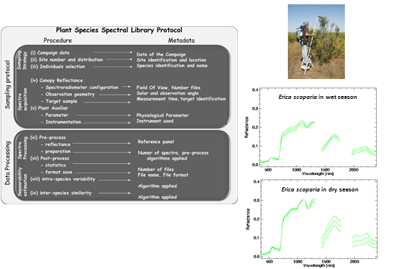
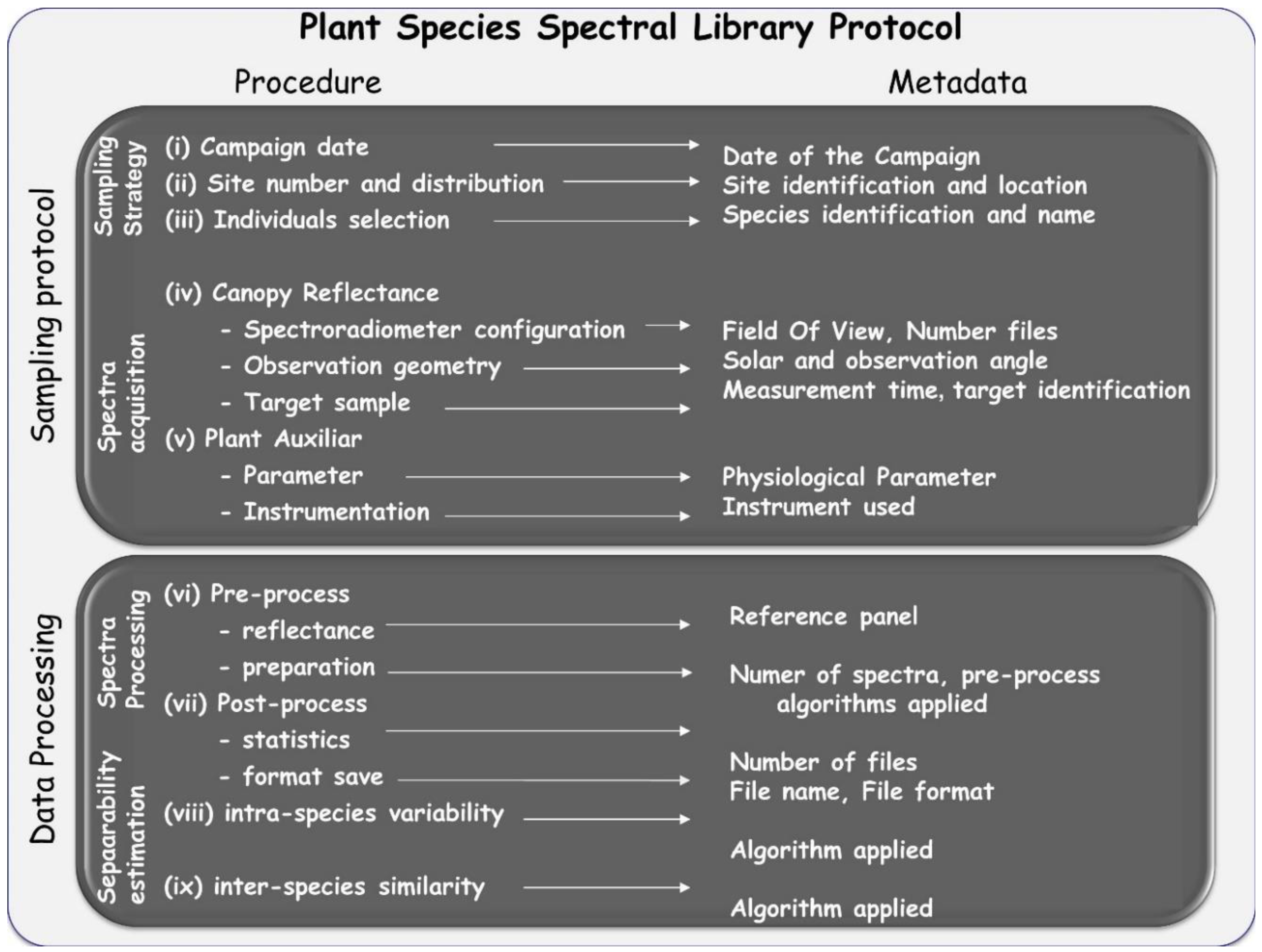
3. Plant Spectral Library Protocol

3.1. Sampling Protocol
- (i)
- Field campaign dates should cover the phenological stages of the different species and identify seasonal differences in leaf aging, leaf drop, flowering and fruiting, and processes that affect relative proportions and the structural arrangement of chemicals exposed to the sensor over time. Depending on the plant community considered, two to four different dates throughout the year may be required to characterize spectral variation.
- (ii)
- The number of measurement sites and their spatial distribution has to cover the different plant communities presented, and should be stratified to account for environmental gradients (i.e., soil type, topography). Stratified areas might be easily identified by using ancillary vegetation and topography maps of the study area, taking into account the extent of the area and its accessibility (i.e., marshlands or very dense vegetation). The size of the measurement site is not relevant because the aim of the spectral library is the characterization of the species signature and endmember generation.
- (iii)
- The individuals to be measured may be selected by random sampling, but selected individuals should represent the “normal” state of the plant species and avoid damaged, sick, or juvenile individuals. The total number of individuals will be a function of the number of the definitive sampling sites, after the stratification process is completed. Several more individuals may be selected for plant communities with marked heterogeneity related to the environmental gradients observed. As an overall recommendation, at least 30 individuals are required for statistical reasons [41].
- (iv)
- In selecting and configuring the field spectroradiometer, the vegetation type must be considered. For instance, to accomplish lignin and cellulose absorption bands presented in woody species the field spectroradiometer should have sensing capabilities for the SWIR region [10]. For the appropriate determination of observation geometry, the instrument’s FOV should be broad enough to include every constituent of the canopy, capturing the entire size of tree canopies, shrubs or forbs by using poles, ladders, or cranes. However, the FOV should not be too large as to prevent signals from external elements around the measured plant. To select observation angles, nadiral sampling is suggested in order to avoid hotspot effects. The whole canopy has to be sampled moving the spectroradiometer’s head within the canopy, recording various files per measurement to account for canopy variability. At this point, depending on the spectroradiometer used, attention must be paid to the actual pixel size with the fore-optic or fiber optic applied [42]. As recommended in general field spectroscopy protocols [43], the measurement time must be as close as possible to solar noon. For plant spectra acquisition, a field spectroradiometer could be configured to acquire radiance or DN mode. After field spectroradiometer optimization, the radiance of the reference panel and plant canopy are registered. In order to minimize the variation in the output plant reflectance due to changes in solar illumination, the canopy and calibration panel radiance and sensor dark current should be measured nearly simultaneously.
- (v)
- The measurement of physicochemical parameters for the sampled individuals during spectral acquisition is strongly recommended. A vast amount of literature for this physiological parameter acquisition on site is available. For example, Jonckheere et al. [44] review several direct and indirect methods for LAI estimation. Methods for chlorophyll content or leaf water content measurements can be found in Gitelson [45] and Colombo et al. [46], respectively.
3.2. Data Processing and Spectral Separability Calculations
- (vi)
- Field spectroradiometers usually have the option to register target and reference panel radiance measurements either jointly in the same file or in separate files. It is important to be aware that spectral data is usually saved in a proprietary format, which can only be read by specific software distributed by the manufacturer. Depending on the spectral noise level, polishing techniques, such as the Savitzky-Golay filter, might be applied but it is advisable to be conservative for the sake of preserving information [47]. In addition, it is also possible to apply spectral transformation (i.e., continuum-removed, derivative). Similarly, all metadata on spectral acquisition should be addressed, by identifying the metadata source and data type: for example, recording information about the configuration of the spectroradiometer in the file, or saving a picture of the sampled plant species.
- (vii)
- During post-processing of spectra, the average reflectance and standard deviation are calculated for every measurement of the same target. To make data available for the scientific community, a common file format can be used: ASCII, Hierarchical Data File (HDF), jcamp-dx, or commercial imaging software format like the ENVI spectral library (Exelis Visual Information Solutions, Inc., Boulder, CO, USA). Similarly, metadata files should be generated and appended to the spectral library in a widely used and standard format. In this respect, Jimenez et al. [23] have suggested writing metadata files in Extensible Markup Language (XML) following international standards.
- (viii)
- Intra-species spectra variability may be checked based on the different phenological states and physiochemical parameters. The coefficient of variation (CV) or simple least square regression are statistical techniques that help to identify sensitive wavelength. In addition, univariate and multivariate statistical techniques, including both parametric and non-parametric analysis of variance, can aid in the comparison of the spectral response over the different measurement dates in order to identify in which season the species easily discriminate from each other.
- (ix)
- The inter-species similarity index [11] can provide an estimation of differences in the spectral signature of plant species. In order not to losepossible subtle differences between species spectra, the protocol proposes the use of two different separability metrics for comparison, both applied either to the original and to the continuum-removed spectra.
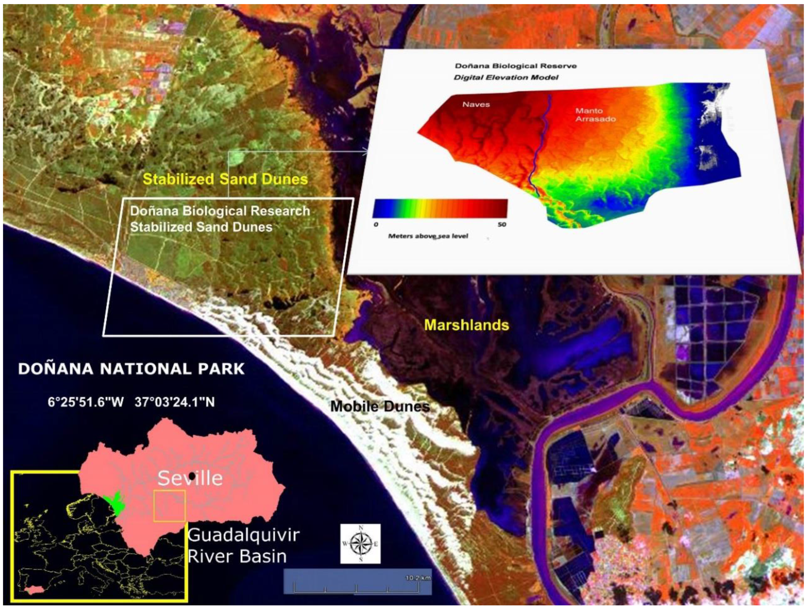
4. Case Study: Shrublands of Doñana National Park
4.1. Study Area
4.2. Shrub Species Spectral Library

| Plant Physiochemical Parameters | Erica scoparia | Halimium halimifolium | Rosmarinus officinalis | Stauracanthus genistoides | Ulex australis |
|---|---|---|---|---|---|
 |  | 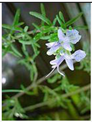 | 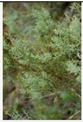 | 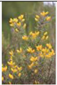 | |
| Family | Ericaceae | Cistaceae | Lamiaceae | Leguminosae | Leguminosae |
| Common name | Brezo de escobas | Jaguarzo blanco | Romero | Tojo Morisco | Tojo |
| Leaf type | Schlerophyll | Semi-Schlerophyll | Semi-Schlerophyll | spines | spines |
| Average Height | 100 cm–3 m | 60–150 cm | 100–150 m | 60–100 cm | 60–100 cm |
| Canopy Diameter | 1–2 m | 50–100 cm | 50–100 cm | 50–100 cm | 50–100 cm |
| Regeneration | roots | seeds | Seeds | roots | roots |
| Root morphology | Horizontal | Horizontal / vertical | Horizontal | Horizontal/vertical | Horizontal/vertical |
| Leaf water potential | −3.0 Mpa | −4.0 Mpa | −11.0 Mpa | −1.7 Mpa | −2.7 Mpa |
- (i)
- To determine field campaign dates, we took into account the very sharp differences in water availability between the wet and dry seasons in DNP. Therefore, in 2006 and 2007, several field spectroscopy campaigns were carried out with measurements collected during the end of the dry season (late March and early April) and the end of the wet season (late August and early September). In the wet season campaigns, no measurements were taken during the flowering period of the Doñana shrubland, which takes place mainly between May and June.
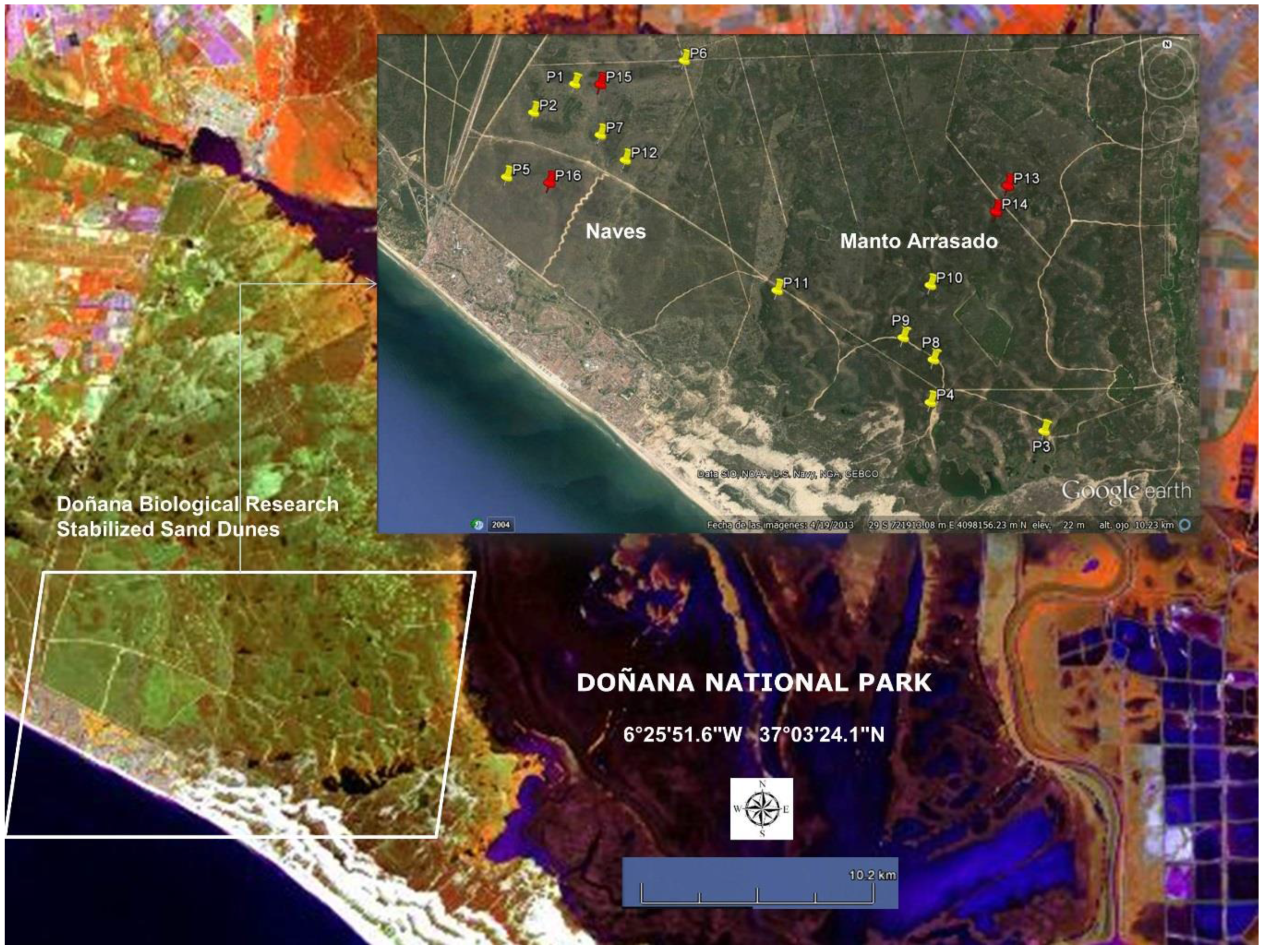
- (ii)
- In the stabilized sand dune ecosystem, micro-topography is the major factor conditioning the sampling stratification. A 10 m pixel digital elevation model and the DBR Ecological Map were used for the stratification of the study area. To select sites along the stratified areas, locations for plant spectral acquisition and LAI measurements were determined using maps, but the choice was constrained by proximity to pathways due to the great difficulty of accessing areas with dense vegetation. A total of 16 measurement sites were selected, 12 of them intended for the acquisition of spectral signatures, while in the four other sites spectral signatures were acquired together with LAI measurements. Figure 3 shows sampling sites distribution, eight of those were located in the Naves, and the other eight sites in Manto Arrasado.
- (iii)
- Two types of canopy spectral measurements with two different aims were recorded: type (I) in order to generate spectral libraries for the five dominant species, 30 individuals for every dominant species were non-randomly selected covering the LAI ranges presented in the stabilized sand dune ecosystems. These measurements were carried out in spectral signature and LAI measurement sites (red tacks in Figure 3) and the individuals were marked and measured in wet and dry seasons; type (II) in order to calculate the spectral variability among the most abundant shrub species, canopy spectral reflectance was also measured for the five dominant species and other abundant shrub species (Lavandula stoechas, Thymus mastichina, Cistus libanotis, Halimium commutatum, Phylirrea angustifilia). These measurements were carried out in spectral signature sites (yellow tacks in Figure 3) only in the dry season and for 30 randomly selected individuals in every species; damaged or individuals in early growing stages were avoided.

- (iv)
- Shrub species have a considerable woody part, which recommended the use of a spectroradiometer with a SWIR detector. The field spectroradiometer chosen was the ASD FieldSpec3 (Analytical Spectral Devices, Boulder, CO, USA), which measures incoming radiance using a fiber optic which is adaptable with a fore optic lens. It has a spectral range from 350 to 2500 nm with a 3 nm spectral resolution and a sampling interval of 1.4 nm in the VNIR spectral regions and 10 nm and 2 nm in the SWIR. Measurements were acquired directly with the fiber optic (FOV 25°) with no fore-optics mounted. The fiber was nadir-oriented and held 1 m above the canopy (GIFOV = 44 cm). For tall individuals a leader was used to maintain a constant distance between the fiber and canopy. Target and reference panel radiance were alternatively acquired and the instrument’s dark current was measured before each sampling. At least five files per plant, averaging five spectra per file, were recorded on a whole sweep of the canopy. During sweeping the pistol grip was continuously turned clockwise and counter-clockwise to minimize spectral misalignments of the ASD fiber [42]. Measurements were concentrated in two hours around noon. The field campaigns were always carried out under cloudless skies.
- (v)
- LAI measurements were carried out in some individuals at the same time as the reflectance spectral acquisitions. We used an indirect method and took hemispherical canopy pictures for each plant. These 180° pictures were always taken from beneath the canopy looking upwards with a NIKON FC-E8 fisheye lens adapted to a Nikon 4000 Coolpix digital camera. The pictures were always gathered at nearly sunset [53]. In this process, the Plant Area Index (PAI) which also includes non-photosynthetic elements, such as branches, was estimated instead of the LAI. The PAI was calculated by processing the corresponding hemispherical canopy picture with Hemiview® 2.1 (Delta-T Devices, Ltd., Cambridge, UK). This software estimates gap fraction over the entire picture and calculates the PAI. In Figure 3, the sites for the PAI measurements are indicated with red tacks.
- (vi)
- Spectral files acquired using ASD Fieldspec3 were imported to ASCII format using ViewSpec® software. Canopy reflectance per plant (five measurements) was calculated by dividing target and reference panel radiance. All collected spectra were parabolic-corrected for the spectroradiometer sensitivity drift at the junctions of the spectral regions of the three different detectors. No spectral polishing algorithm was applied.
- (vii)
- For each plant individual, an average reflectance spectral signature and standard deviation (SD) file was generated. Spectral reflectance at wavelengths of around 1400 nm, 1940 nm, and 2400 nm were excluded due to the presence of excessive noise caused by atmospheric water absorption. The output file was saved in the ENVI spectral library format (Exelis Visual Information Solutions, Inc., Boulder, CO, USA).
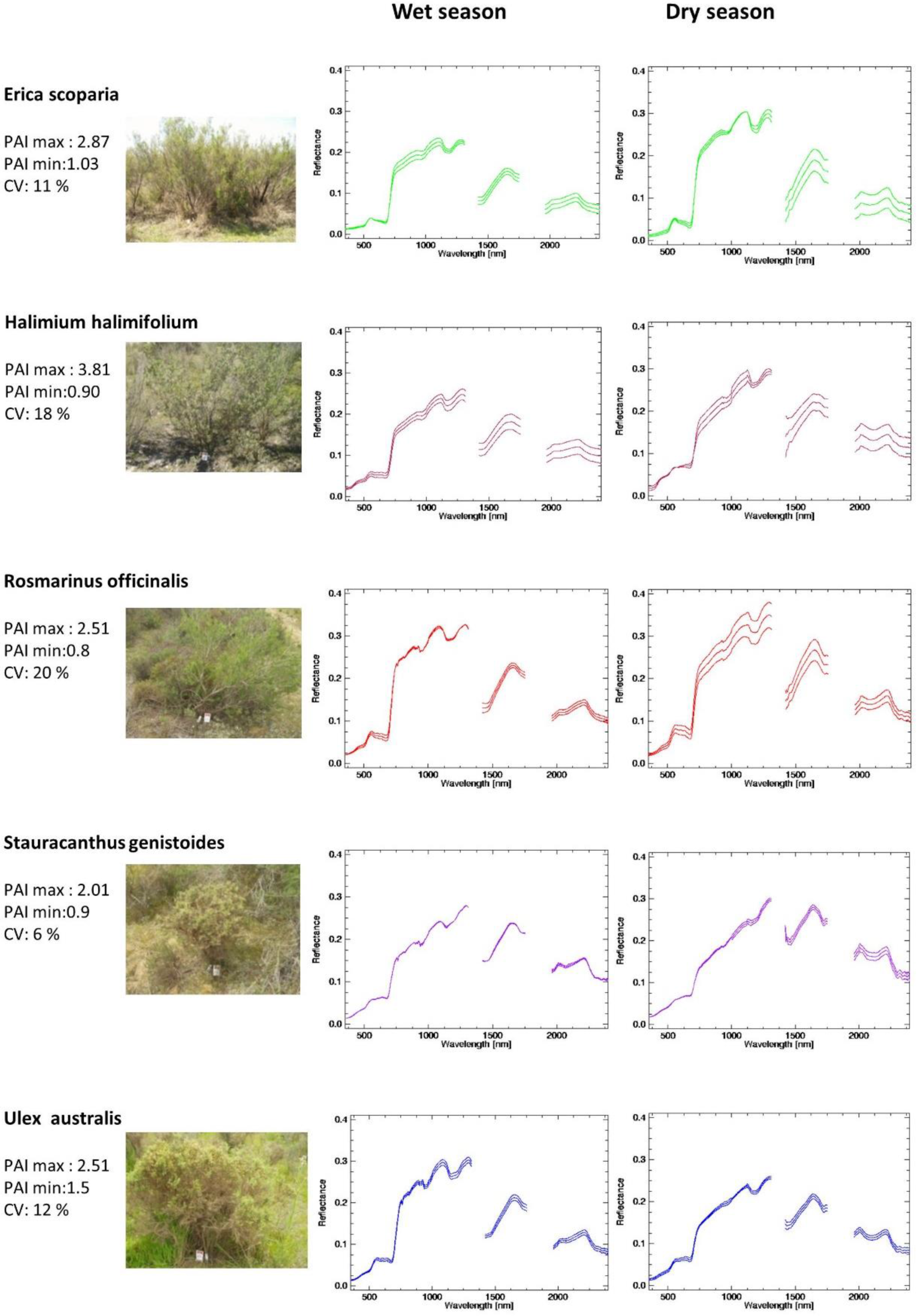
- (viii)
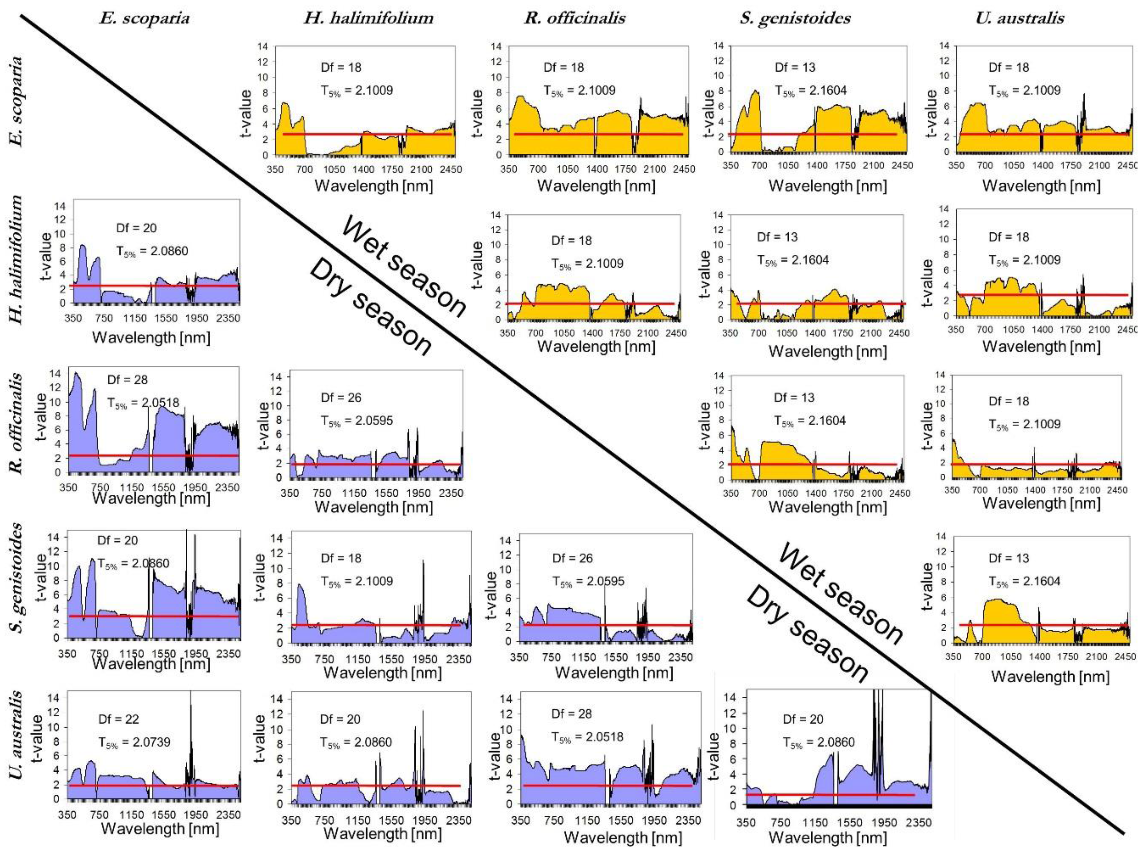
- Once the canopy reflectance spectra for every plant individual was calculated, the spectral library for the five dominant species were generated using the spectra from Type-I measurements. The species coefficient of variation (CV) in dry season was calculated using the spectra for which PAI was measured. CV was calculated for every wavelength and an averaged value was calculated for the entire spectral region. To determine the season when dominant species show greatest variability and most differences between each other, parametrical statistical tests were applied to compare species of Type-I measurement per season. A standard series of two-group t-tests were performed for every wavelength to test the null hypothesis that there were no significant differences between means. This test allows for the identification of the wavelength region where the species show higher spectral separability. Normality was previously explored and confirmed with the Kolmogorov–Smirnov normality test.
- (ix)
- Similarity indexes between species were calculated. In this case, global similarity methodologies were applied on Type-II measurements. Two deterministic algorithms were calculated using the original and continuum-removal algorithm applied to entire spectra. These two algorithms were the Spectral Similarity Value (SSV) [54] and SAM. SSV takes into account curve shapes by comparing correlation and separation calculated by Euclidean distance. By definition, the spectral similarity scale has a minimum of 0 and a maximum of the square root of 2. Low values in the similarity scale indicate similar spectra. SAM calculates the angular distance between two reflectance vectors across wavelengths, and is less sensitive to the amplitude of both spectra. Range values vary from 0 to π/2, where a lower SAM angle means a higher similarity between two spectra.
5. Results
5.1. Dominant Species Spectral Library

5.2. Intra-Species Variability

5.3. Inter-Species Similarity
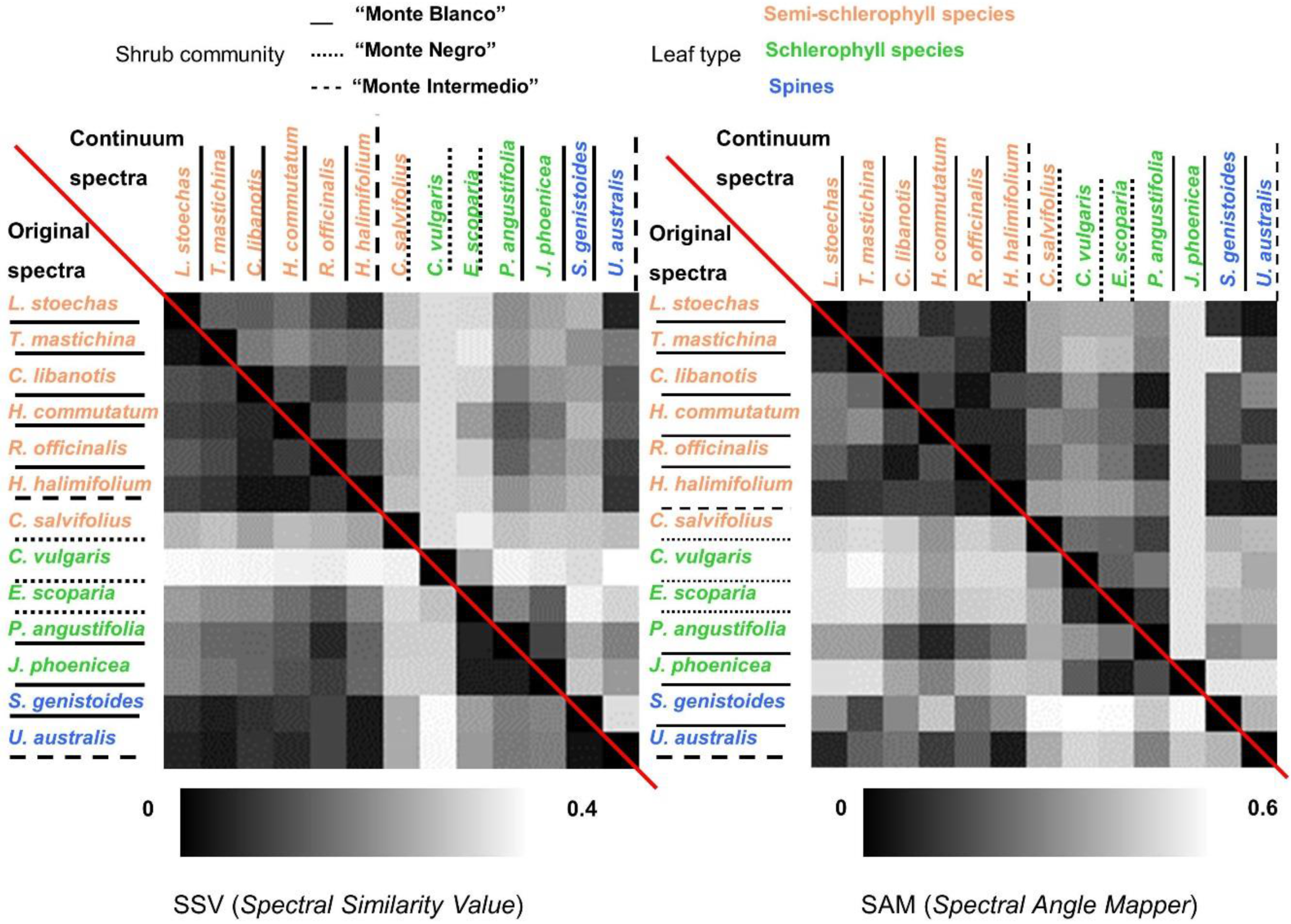
5.3.1. Leaf Type Comparison: within and between Leaf Type Groups
5.3.2. Within and between-Communities Species Comparison
5.3.3. Comparison within Dominant Species
6. Discussion
7. Conclusions
Acknowledgments
Author Contributions
Conflicts of Interest
References
- Schmeller, D.S. European species and habitat monitoring: where are we now? Biodivers. Conserv. 2008, 17, 3321–3326. [Google Scholar] [CrossRef]
- He, K.S.; Rocchini, D.; Neteler, M.; Nagendra, H. Benefits of hyperspectral remote sensing for tracking plant invasions. Divers. Distrib. 2011, 17, 381–392. [Google Scholar] [CrossRef]
- Ustin, S.; Zarco Tejada, P.; Jacquemoud, S.; Asner, G. Remote sensing of environment: State of the science and new directions. In Remote Sensing for Natural Resources Management and Environmental Monitoring. Manual of Remote Sensing, 3rd ed.; Ustin, S.L., Ed.; John Wiley & Sons, Inc.: Hoboken, NJ, USA, 2004; Volume 4, pp. 679–729. [Google Scholar]
- Schaepman, M.E.; Ustin, S.L.; Plaza, A.J.; Painter, T.H.; Verrelst, J.; Liang, S. Earth system science related imaging spectroscopy—An assessment. Remote Sens. Environ 2009, 113, 123–137. [Google Scholar] [CrossRef]
- Kaufmann, H.; Segl, K.; Kuester, T.; Rogass, C.; Foerster, S.; Wulf, H.; Hofer, S.; Sang, B.; Storch, T.; Mueller, A.; et al. The Environmental Mapping and Analysis Program (EnMAP)—Present status of preparatory phase. In Proceedings of the International Geoscience and Remote Sensing Symposium (IAGARSS’13), Melbourne, Australia, 21–26 July 2013.
- Romano, F.; Santini, F.; Simoniello, T.; Ananasso, C.; Corsini, G.; Cuomo, V. The PRISMA hyperspectral mission: Science activities and opportunities for agriculture and land monitoring. In Proceedings of the International Geoscience and Remote Sensing Symposium (IGARSS’13), Melbourne, Australia, 21–26 July 2013.
- Milton, E.J.; Schaepman, M.E.; Anderson, K.; Kneubühler, M.; Fox, N. Progress in field spectroscopy. Remote Sens. Environ. 2009, 113, 92–109. [Google Scholar] [CrossRef]
- Asner, G.P.; Jones, M.O.; Martin, R.E.; Knapp, D.E.; Hughes, R.F. Remote sensing of native and invasive species in Hawaiian rainforests. Remote Sens. Environ. 2008, 112, 1912–1926. [Google Scholar] [CrossRef]
- Lewis, M.M. A strategy for mapping arid vegetation associations with hyperspectral imagery. In Proceedings of Eleventh Australian Remote Sensing and Photogrammetry Conference, Brisbane, Australia, 2–6 September 2002; pp. 647–655.
- Asner, G.P. Biophysical and biochemical sources of variability in canopy reflectance. Remote Sens. Environ. 1998, 64, 234–253. [Google Scholar] [CrossRef]
- Clark, M.L.; Roberts, D.A. Species-level differences in hyperspectral metrics among tropical rainforest trees as determined by a tree-based classifier. Remote Sens. 2012, 4, 1820–1855. [Google Scholar] [CrossRef]
- Warner, T.A. Remote sensing analysis: From project design to implementation. In Manual of Geospatial Sciences, 2nd ed.; Bossler, J.D., McMaster, R.B., Rizos, C., Campbell, J.B., Eds.; Taylor and Francis: London, UK, 2010; Chapter 17; pp. 301–318. [Google Scholar]
- Manakos, I.; Manevski, K.; Petropoulos, G.P.; Elhag, M.; Kalaitzidis, C. Development of a spectral library for Mediterranean land cover types. In Proceedings of 30th EARSeL Symp.: Remote Sensing for Science, Education and Natural and Cultural Heritage, Paris, France, 31 May–3 June 2010; pp. 663–668.
- Zomer, R.J.; Trabucco, A.; Ustin, S.L. Building spectral libraries from wetlands land cover classification and hyperspectral remote sensing. J. Environ. Manag. 2008, 90, 2170–2177. [Google Scholar] [CrossRef] [PubMed]
- Ruby, J.G.; Fischer, R.L. Spectral signatures database for remote sensing applications. Proc. SPIE 2002, 4816, 156–163. [Google Scholar]
- Hueni, A.; Malthus, T.; Kneubuehler, M.; Schaepman, M. Data exchange between distributed spectral databases. Comput. Geosci. 2011, 37, 861–873. [Google Scholar] [CrossRef]
- Pfitzner, K.; Bollhöfer, A.; Esparon, A.; Bartolo, B.; Staben, G. Standardized spectra (400–2500 nm) and associated metadata: An example from northern tropical Australia. In Proceedings of IEEE International Geoscience and Remote Sensing Symposium, Honolulu, Hawaii, USA, 25–30 July 2010.
- Buddenbaum, H.; Stern, O.; Stellmes, M.; Stoffels, J.; Pueschel, P.; Hill, J.; Werner, W. Field Imaging spectroscopy of beech seedlings under dryness stress. Remote Sens. 2012, 4, 3721–3740. [Google Scholar] [CrossRef]
- Hruska, R.; Mitchell, J.; Anderson, M.; Glenn, N.F. Radiometric and geometric analysis of hyperspectral imagery acquired from an unmanned aerial vehicle. Remote Sens. 2012, 4, 2736–2752. [Google Scholar] [CrossRef]
- Nidamanuri, R.R.; Zbell, B. Use of field reflectance data for crop mapping using airborne hyperspectral image. ISPRS J. Photogramm. Remote Sens. 2011, 66, 683–691. [Google Scholar] [CrossRef]
- Hueni, A.; Nieke, J.; Schopfer, J.; Kneubühler, M.; Itten, K.I. The spectral database SPECCHIO for improved long-term usability and datasharing. Comput. Geosci. 2009, 35, 557–565. [Google Scholar] [CrossRef] [Green Version]
- Rasaiah, B.; Jones, S.; Bellman, C.; Malthus, T.J. Critical metadata for spectroscopy field campaigns. Remote Sens. 2014, 6, 3662–3680. [Google Scholar] [CrossRef]
- Jiménez, M.; González, M.; Amaro, A.; Fernández-Renau, A. Field spectroscopy metadata system based on ISO and OGC standards. ISPRS Int. J. Geo-Inf. 2014, 3, 1003–1022. [Google Scholar] [CrossRef]
- Nicodemus, F.E.; Richmond, J.C.; Hsia, J.J.; Ginsberg, I.W.; Limperis, T. Geometrical Considerations and Nomenclature for Reflectance; National Bureau of Standards, US Department of Commerce: Washington, DC, USA, 1977. [Google Scholar]
- Thenkabail, P.; Lyon, J.; Huete, A. Advances in hyperspectral remote sensing of vegetation and agricultural croplands. In Hyperspectral Remote Sensing of Vegetation; Thenkabail, P.S., Lyon, J.G., Huete, A., Eds.; CRC Press/Taylor and Francis Group: Boca Raton, FL, USA, 2011; pp. 3–36. [Google Scholar]
- Miao, X. Estimation of yellow starthistle abundance through CASI-2 hyperspectral imagery linear spectral mixture models. Remote Sens. Environ. 2006, 101, 329–341. [Google Scholar] [CrossRef]
- Möckel, T.; Dalmayne, J.; Prentice, H.C.; Eklundh, L.; Purschke, O.; Schmidtlein, S.; Hall, K. Classification of grassland successional stages using airborne hyperspectral imagery. Remote Sens. 2014, 6, 7732–7761. [Google Scholar] [CrossRef]
- Roberts, D.A.; Gardner, M.; Church, R.; Ustin, S.; Scheer, G.; Green, R.O. Mapping chaparral in the Santa Monica mountains using multiple endmember spectral mixture models. Remote Sens. Environ. 1998, 65, 267–279. [Google Scholar] [CrossRef]
- Manevski, K.; Manakosa, I.; Petropoulosa, P.; Kalaitzidis, C. Discrimination of common Mediterranean plant species using field spectroradiometry. Int. J. Appl. Earth Obs. Geoinf. 2011, 13, 922–933. [Google Scholar] [CrossRef]
- Silvestry, S.; Marani, M.; Marani, A. Hyperspectral remote sensing of salt marsh vegetation. Phys. Chem. Earth. 2003, 28, 15–25. [Google Scholar] [CrossRef]
- Kalacska, M. Ecological fingerprinting of ecosystem succession: Estimating secondary tropical dry forest structure and diversity using imaging Spectroscopy. Remote Sens. Environ. 2007, 108, 82–96. [Google Scholar] [CrossRef]
- Somers, B.; Asner, G.P. Hyperspectral time series analysis of native and invasive species in Hawaiian rainforests. Remote Sens. 2012, 4, 2510–2529. [Google Scholar] [CrossRef]
- Fyfe, S.K. Spatial and temporal variation in spectral reflectance: Are seagrass species spectrally distinct? Limnol. Oceanogr. 2003, 464–479. [Google Scholar] [CrossRef]
- SPECCHIO. Online Spectral Database. Available online: http://www.specchio.ch (accessed on 11 August 2015).
- Clark, R.N.; Roush, T.L. Reflectance spectroscopy: Quantitative analysis techniques for remote sensing applications. J. Geophys. Res. 1984, 89, 6329–6340. [Google Scholar] [CrossRef]
- Price, J.C. How unique are spectral signatures? Remote Sens. Environ. 1994, 49, 181–186. [Google Scholar] [CrossRef]
- Jacquemoud, S.; Verhoef, W.; Baret, F.; Bacour, C.; Zarco-Tejada, P.J.; Asner, G.P.; Francois, C.; Ustin, S.L. PROSPECT + SAIL models: A review of use for vegetation characterization. Remote Sens. Environ. 2009, 113, S56–S66. [Google Scholar] [CrossRef]
- Homayouni, S.; Roux, M. Hyperspectral Image analysis for material mapping using spectral matching. In Proceedings of ISPRS Congress 2004, Istanbul, Turkey, 12–23 July 2004.
- Kruse, F.A.; Lefkoff, A.B.; Boardman, J.B.; Heidebrecht, K.B.; Shapiro, A.T.; Barloon, P.J.; Goetz, A.F.H. The Spectral Image Processing System (SIPS)—Interactive visualization and analysis of imaging spectrometer data. Remote Sens. Environ. 1993, 44, 145–163. [Google Scholar] [CrossRef]
- International Organization for Standardization (ISO). Geographic Information—Metadata; International Organization for Standardization: Geneva, Switzerland, 2003. [Google Scholar]
- Mac Arthur, A.; Alonso, L.; Malthus, T.; Moreno, J. Spectroscopy field strategies and their effect on measurements of heterogeneous and homogeneous earth surfaces. In Proceedings of the 2013 Living Planet Symposium, Edinburgh, UK, 9–13 September 2013.
- Mac Arthur, A.; MacLellan, C.; Malthus, T.J. The fields of view and directional response functions of two field spectroradiometers. IEEE Trans. Geosci. Remote Sens. 2012, 50, 3892–3907. [Google Scholar] [CrossRef]
- Salisbury, J.W. Spectral Measurements Field Guide; Tech. Rep. ADA362372; Defense Technology Information Centre: Fort Belvoir, VA, USA, 1998. [Google Scholar]
- Jonkheere, I.; Fleck, S.; Nackaerts, K.; Muys, B.; Coppin, P.; Weiss, M.; Baret, F. Review of in-situ methods of leaf area index determination. Part I. Theories, sensors and hemispherical photography. Agric. For. Meteorol. 2004, 121, 19–35. [Google Scholar] [CrossRef]
- Gitelson, A.A. Nondestructive estimation of foliar pigment (chlorophylls, carotenoids, and anthocyanins) contents. In Hyperspectral Remote Sensing of Vegetation; Thenkabail, A., Lyon, P.S., Huete, J.G., Eds.; CRC Press: Boca Raton, FL, USA, 2011; pp. 141–166. [Google Scholar]
- Colombo, R.; Busetto, L.; Meroni, M.; Rossini, M.; Panigada, C. Optical remote sensing of vegetation water content. In Hyperspectral Remote Sensing of Vegetation; Thenkabail, A., Lyon, P.S., Huete, J.G., Eds.; CRC Press: Boca Raton, FL, USA, 2011; pp. 227–244. [Google Scholar]
- Schmidt, K.S.; Skidmore, A.K. Smoothing vegetation spectra with wavelets. Int. J. Remote Sens. 2004, 25, 1167–1184. [Google Scholar] [CrossRef]
- García Novo, F.; Marín Cabrera, C. Doñana: Agua y Biosfera; Ministerio de Medio Ambiente: Sevilla, España, 2005. [Google Scholar]
- Muñoz Reinoso, J.C.; García Novo, F. Multiscale control of vegetation patterns: The case of Doñana (SW Spain). Lands. Eco. 2005, 20, 51–61. [Google Scholar] [CrossRef]
- Zunzunegui, M.; Díaz Barradas, M.C.; Ain-Lhout, F.; Clavijo, A.; García Novo, F. To live or to survive in Doñana dunes: Adaptive responses of woody species under a Mediterranean climate. Plant Soil 2005, 273, 77–89. [Google Scholar] [CrossRef]
- Gratani, L.; Varone, L. Adaptive photosynthetic strategies of the Mediterranean maquis species according to their origin. Photosynthetica 2004, 42, 551–558. [Google Scholar] [CrossRef]
- Ain-Lhout, F. Seasonal differences in photochemical efficiency and chlorophyll and carotenoid contents in six Mediterranean shrub species under field conditions. Photosynthetica 2004, 42, 309–407. [Google Scholar] [CrossRef]
- Chen, J.M.; Cihlar, J. Quantifying the effect of canopy architecture on optical measurements of leaf area index using two gap size analysis methods. IEEE Trans. Geosci. Remote Sens. 1994, 33, 777–787. [Google Scholar] [CrossRef]
- Sweet, J.; Granahan, J.; Sharp, M. An objective standard for hyperspectral image quality. In Proceedings of AVIRIS Workshop, Jet Propulsion Laboratory, Pasadena, CA, USA, 23–25 February 2000.
- Jimenez, M.; Pou, A.; Díaz-Delgado, R. Cartografía de especies de matorral de la Reserva Biológica de Doñana mediante el sistema hiperespectral aeroportado INTA-AHS: Implicaciones en el seguimiento y estudio del matorral de Doñana. Revis. de Teledetec. 2011, 36, 98–102. [Google Scholar]
© 2015 by the authors; licensee MDPI, Basel, Switzerland. This article is an open access article distributed under the terms and conditions of the Creative Commons Attribution license (http://creativecommons.org/licenses/by/4.0/).
Share and Cite
Jiménez, M.; Díaz-Delgado, R. Towards a Standard Plant Species Spectral Library Protocol for Vegetation Mapping: A Case Study in the Shrubland of Doñana National Park. ISPRS Int. J. Geo-Inf. 2015, 4, 2472-2495. https://doi.org/10.3390/ijgi4042472
Jiménez M, Díaz-Delgado R. Towards a Standard Plant Species Spectral Library Protocol for Vegetation Mapping: A Case Study in the Shrubland of Doñana National Park. ISPRS International Journal of Geo-Information. 2015; 4(4):2472-2495. https://doi.org/10.3390/ijgi4042472
Chicago/Turabian StyleJiménez, Marcos, and Ricardo Díaz-Delgado. 2015. "Towards a Standard Plant Species Spectral Library Protocol for Vegetation Mapping: A Case Study in the Shrubland of Doñana National Park" ISPRS International Journal of Geo-Information 4, no. 4: 2472-2495. https://doi.org/10.3390/ijgi4042472
APA StyleJiménez, M., & Díaz-Delgado, R. (2015). Towards a Standard Plant Species Spectral Library Protocol for Vegetation Mapping: A Case Study in the Shrubland of Doñana National Park. ISPRS International Journal of Geo-Information, 4(4), 2472-2495. https://doi.org/10.3390/ijgi4042472