Article

Image Segmentation Parameter Optimization Considering Within- and Between-Segment Heterogeneity at Multiple Scale Levels: Test Case for Mapping Residential Areas Using Landsat Imagery
by
Brian A. Johnson
1,*,
Milben Bragais
2,
Isao Endo
1,
Damasa B. Magcale-Macandog
2 and
Paula Beatrice M. Macandog
2
1
Institute for Global Environmental Strategies, 2108-11 Kamiyamaguchi, Hayama, Kanagawa 240-0115, Japan
2
Institute of Biological Sciences, University of the Philippines Los Baños, College, Laguna 4031, Philippines
*
Author to whom correspondence should be addressed.
ISPRS Int. J. Geo-Inf. 2015, 4(4), 2292-2305; https://doi.org/10.3390/ijgi4042292
Submission received: 2 September 2015 / Revised: 15 October 2015 / Accepted: 15 October 2015 / Published: 27 October 2015

Abstract

:
Multi-scale/multi-level geographic object-based image analysis (MS-GEOBIA) methods are becoming widely-used in remote sensing because single-scale/single-level (SS-GEOBIA) methods are often unable to obtain an accurate segmentation and classification of all land use/land cover (LULC) types in an image. However, there have been few comparisons between SS-GEOBIA and MS-GEOBIA approaches for the purpose of mapping a specific LULC type, so it is not well understood which is more appropriate for this task. In addition, there are few methods for automating the selection of segmentation parameters for MS-GEOBIA, while manual selection (i.e., trial-and-error approach) of parameters can be quite challenging and time-consuming. In this study, we examined SS-GEOBIA and MS-GEOBIA approaches for extracting residential areas in Landsat 8 imagery, and compared naïve and parameter-optimized segmentation approaches to assess whether unsupervised segmentation parameter optimization (USPO) could improve the extraction of residential areas. Our main findings were: (i) the MS-GEOBIA approaches achieved higher classification accuracies than the SS-GEOBIA approach, and (ii) USPO resulted in more accurate MS-GEOBIA classification results while reducing the number of segmentation levels and classification variables considerably.

1. Introduction

Fine-scale population data is needed for assessing vulnerability to various natural hazards, e.g., for estimating the number of people living in a flood-prone area [1]. To obtain this fine-scale data, “dasymetric mapping” techniques are often used to downscale population counts and/or other demographic data from census units (e.g., block-group, neighborhood, city) to the scale of an ancillary data set [2]. A gridded map of residential (i.e., populated) and non-residential (i.e., unpopulated) areas is the ancillary data source for the most commonly-used dasymetric mapping method, the grid binary method [3], which involves evenly distributing the population (or other demographic statistics) of a census unit to residential areas within the census unit. Accurate and up-to-date residential/non-residential area maps are therefore important for supporting vulnerability assessments.
Residential areas can be extracted from remote sensing imagery, but because they tend to be spectrally heterogeneous, containing a mix of built-up land (which itself consists of many different surface materials) and vegetated land, it is difficult to accurately map them using traditional pixel-based classification methods which consider only the spectral properties of individual pixels [4]. Geographic object-based image analysis (GEOBIA) methods [5], on the other hand, can incorporate textural and contextual information in addition to spectral information for land use/land cover (LULC) classification [6], making them well-suited for mapping residential areas [7]. The first step in GEOBIA is image segmentation, a process that subdivides an image into relatively homogeneous regions (i.e., image segments). LULC classification is then carried out with segments as the base processing units rather than single pixels. Multi-scale/multi-level GEOBIA (MS-GEOBIA) approaches, which incorporate multiple segmentations of an image at different “scale” levels for LULC classification (i.e., different average segment sizes), often outperform single-scale/single-level GEOBIA (SS-GEOBIA) approaches when LULC features of interest differ in size and/or texture [8,9,10,11], as even a very accurate single-level segmentation will likely split some LULC features into multiple segments (i.e., oversegment) and/or group them together with other neighboring LULC features in a single segment (i.e., undersegment). Many MS-GEOBIA studies involve classifying different LULC types at each segmentation level [8,12,13,14,15], while few have compared SS-GEOBIA and MS-GEOBIA approaches for classifying a single LULC type of interest [16]. Residential areas vary in terms of both size (area of residential development) and texture (e.g., building sizes and building densities which vary by development), so a MS-GEOBIA approach may be more appropriate than SS-GEOBIA for mapping them.
Selection of parameters for image segmentation (i.e., parameters that determine the average size and/or shape of segments) can be time-consuming and subjective using visual analysis alone [17], particularly for MS-GEOBIA, as the number of possible combinations of segmentations to use for classification can become very large. For these reasons, automated segmentation parameter optimization (SPO) methods can be particularly useful for MS-GEOBIA. Unsupervised SPO (USPO) algorithms are becoming a popular type of SPO method in remote sensing, and they optimize segmentation parameters based on the spectral and textural properties of image segments. However, the impact of USPO on MS-GEOBIA classification has not been evaluated in detail, and most USPO methods can only be used for SS-GEOBIA.
In this study, we investigated whether an MS-GEOBIA approach and USPO could lead to more accurate mapping of residential areas in Landsat 8 imagery. To our knowledge, this is (1) the first study to compare the performance of SS-GEOBIA and MS-GEOBIA for mapping residential areas, and (2) the first study to evaluate the impact of USPO on MS-GEOBIA classification accuracy by comparing naïve and parameter-optimized classification results. In support of (2), we proposed a USPO method specifically for MS-GEOBIA.

2. Parameter Optimization for SS-GEOBIA and MS-GEOBIA

For both SS-GEOBIA and MS-GEOBIA, segmentation parameters need to be set prior to image segmentation, and the selection of these parameters can have a significant impact on image classification accuracy [18]. SPO methods can generally be divided into supervised SPO (SSPO) and USPO methods. SPO methods require ground-truth polygons of sample objects to be digitized, which can be time-consuming and somewhat subjective in terms of sample object selection (e.g., for MS-GEOBIA, selecting which sample objects to use for optimizing each segmentation level) and boundary delineation. USPO methods, on the other hand, are based solely on image statistics and do not require ground-truth polygons, so their main advantages are their higher levels of objectivity and automation [17]. Here, we focus only on the USPO methods.
Most USPO methods in remote sensing have the goal of identifying a segmentation which maximizes within-segment homogeneity and between-segment heterogeneity [19,20,21,22,23]. Both of these properties are desirable, as high within-segment homogeneity indicates that undersegmentation is not prevalent, while high between-segment heterogeneity indicates that oversegmentation is not prevalent (i.e., segments are spectrally discrete from their neighbors). The previous unsupervised methods that considered both of these properties were designed for SS-GEOBIA (to identify one optimal segmentation) and cannot be applied to MS-GEOBIA in their current forms.
To help solve this problem, we propose some modifications to an existing multi-band USPO method [20] to permit MS-GEOBIA implementation. The existing method measures within-segment homogeneity by the area-weighted variance (WV) of all the segments in a segmentation level [19] and between-segment heterogeneity using Global Moran’s I (MI) [24], a spatial autocorrelation metric which calculates the spectral similarity between segments and their neighbors and then aggregates the results. Lower WV values indicate segmentation levels with higher within-segment homogeneity (i.e., less undersegmentation), while lower MI values indicate segmentation levels with lower spectral similarity between neighboring segments (i.e., less oversegmentation). Here, the WV and MI values are both normalized to a 0–1 range by:
W V n o r m =   X m a x X X m a x X m i n
M I n o r m = X m a x X X m a x X m i n
where W V n o r m is the normalized WV value, M I n o r m is the normalized MI value, X is the WV (or MI) value of the current segmentation, and X m a x and X m i n are the maximum and minimum WV (or MI) values of all the generated segmentations. Higher W V n o r m and M I n o r m values indicate higher undersegmentation and oversegmentation “goodness”, respectively. W V n o r m and M I n o r m values are calculated for each spectral band and then averaged.
Various methods can be used to combine undersegmentation and oversegmentation goodness measures to calculate the “overall goodness” (OG) of each segmentation level, and several examples are given in Zhang et al. [17]. Here, we suggest combining them using the F-measure (F) [25] because a recent study on SSPO by Zhang et al. [26] found that F had greater sensitivity to excessive undersegmentation/oversegmentation than other commonly-used combination methods including addition and Euclidean distance. F is often used for assessing the accuracy of a specific class, and it takes into account false positives (using a “precision” metric) as well as false negatives (using a “recall” metric) to compute a single class-specific accuracy value. In [26], it was instead used to combine precision- and recall-based metrics representing oversegmentation and undersegmentation goodness, respectively, to compute an OG value for each segmentation. Based on this logic, in our study, OG calculated by F (OGf), can be given by:
O G f = ( 1 + a 2 ) M I n o r m   ×   W V n o r m a 2   ×   M I n o r m + W V n o r m
where a is a weight which controls the relative weights of W V n o r m and M I n o r m . For example, a = 1 indicates equal weighting for W V n o r m and M I n o r m , while a = 0.5 indicates half weighting for W V n o r m , and a = 2 indicates double weighting for W V n o r m . O G f values range from 0 to 1, with higher values indicating higher segmentation quality.
Previous USPO studies have used an equal weighting approach for combining undersegmentation and oversegmentation goodness metrics to identify a single optimal segmentation [19,20,21,23,27,28], but we propose that these USPO methods can be also be applied for MS-GEOBIA by adjusting the weights assigned to the undersegmentation and oversegmentation goodness metrics (e.g., by modifying the value of a in Equation (3)). For example, values of a > 1 in Equation (3) may be appropriate for selecting the parameters for finer segmentation levels (to ensure that smaller objects of interest or objects spectrally-similar to their surroundings are not undersegmented at these levels), while values of a < 1 may be more appropriate for selecting parameters for coarser segmentation levels (to ensure that larger/more heterogeneous objects of interest are not oversegmented at these levels). As a simple example, for a two-level GEOBIA approach, undersegmentation goodness ( W V n o r m ) could be given double weighting (a = 2) at segmentation level 1 and half weighting (a = 0.5) at scale level 2.

3. Methods

3.1. Study Area and Data

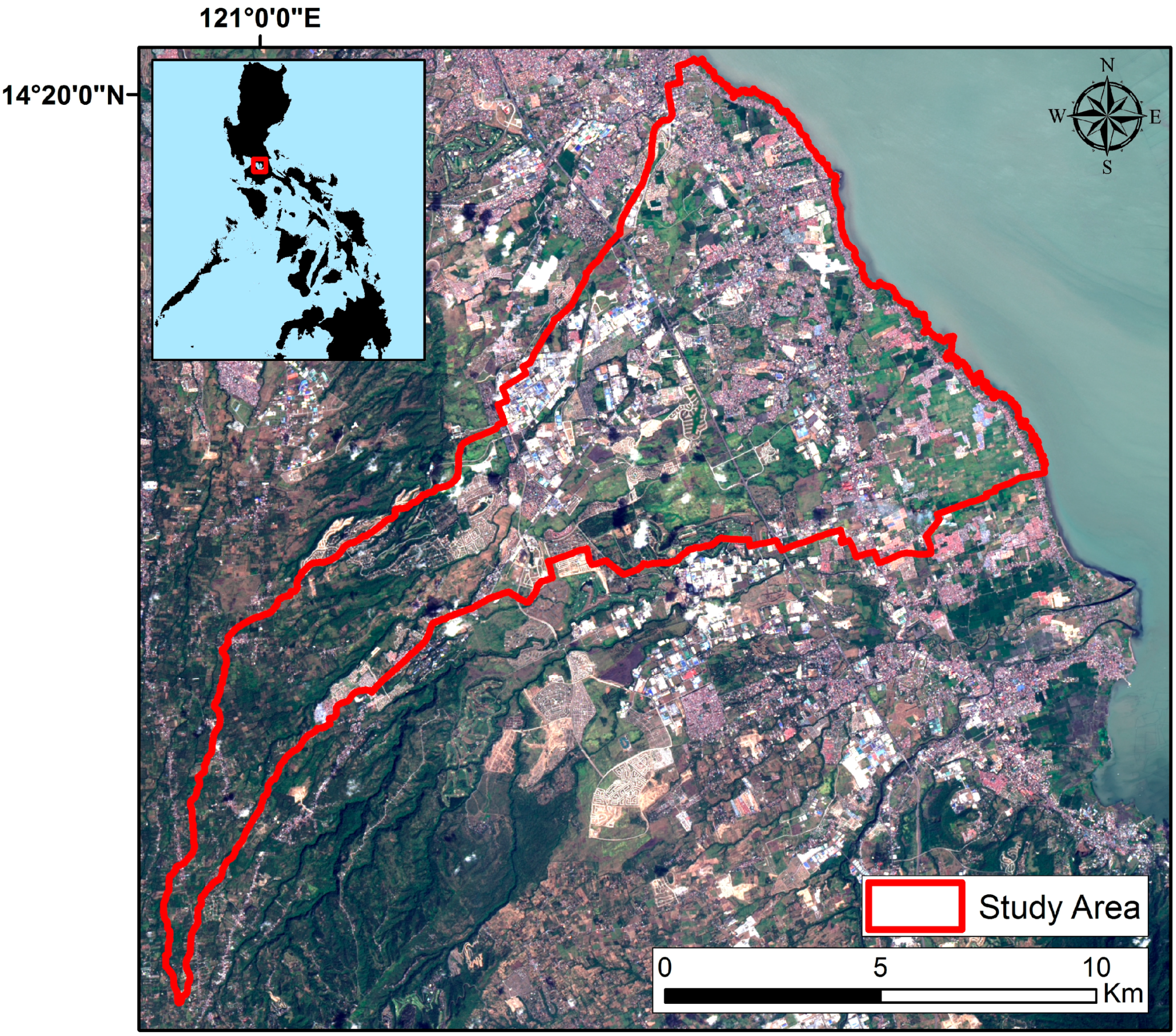
The Silang-Santa Rosa watershed of the Philippines was selected as the study site because it has been undergoing rapid urbanization in recent years, and the local government units needed a fine-scale map of residential areas to conduct flood vulnerability analysis. Landsat 8 imagery of the area, acquired 7 February 2014, was obtained from [29]. The residential areas in the study area consist mainly of detached single-family houses, with building sizes, lot sizes, and building/rooftop materials varying considerably in different developments. The other main LULC types in the watershed include agriculture, agroforestry (coconut plantations), broadleaf forest, idle grassland, light industry, and large commercial facilities (e.g., shopping malls). Figure 1 gives an overview of the study area.
Figure 1. Overview of study area and Landsat 8 satellite imagery (natural color composite).
Ijgi 04 02292 g001

3.2. Image Pansharpening

Since the residential areas did not have a unique spectral signature, and high resolution texture information can be useful for mapping them [7], we improved the spatial resolution of the original Landsat 8 multispectral image bands (bands 2–7) from 30 m to 15 m by pansharpening them using the 15 m panchromatic band (band 8) and the Bayesian Data Fusion algorithm (BDF) [30] included in the open-source software Monteverdi, version 2.0.6. BDF pansharpened images can achieve high spatial quality, which is useful for both image segmentation [31] and texture information extraction [7].

3.3. Image Segmentation Parameter Optimization

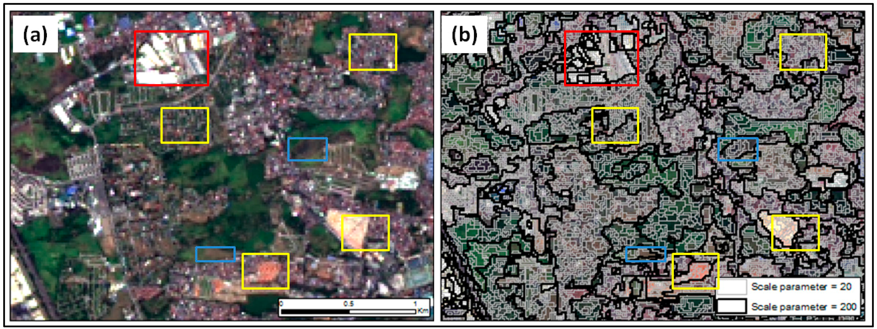
The pansharpened image was segmented in eCognition Developer 8.7 using the multiresolution segmentation algorithm, a region-merging technique with three parameters; a “scale parameter” (SP) which controls the maximum heterogeneity of image segments, a “color/shape” parameter which controls the relative influence of spectral information and shape information, and a “smoothness/compactness” parameter which controls the shape of image segments [14,32]. Here, as in many other GEOBIA studies [8,9,18,33,34], we varied the SP and left the other parameters at their default values. Segmentation was performed for SPs between 20 and 200 using a SP step size of 20. As shown in Figure 2, residential areas were clearly oversegmented at a SP of 20 and undersegmented at a SP of 200, so no SPs <20 or >200 were tested.
Figure 2. (a) Subset of the study area image. (b) segmentation with excessive oversegmentation (gray lines) and excessive undersegmentation (black lines) of residential areas. The yellow boxes show some examples of residential areas with different spectral properties. The red box (industrial area) and blue boxes (bare soil areas) show land use/land cover types with high spectral similarity to residential areas.
Ijgi 04 02292 g002
USPO was done for one-, two-, three-, and four-level segmentations to allow for a detailed comparison between the SS-GEOBIA and MS-GEOBIA approaches. OGf was calculated using the following weights for a:
  • a = 1 for SS-GEOBIA;
  • a = 2 and a = 0.50 for segmentation levels 1–2, respectively, for two-level GEOBIA;
  • a = 3, a = 1, and a = 0.33 for segmentation levels 1–3 for three-level GEOBIA; and
  • a = 4, a = 2, a = 0.50, and a = 0.25 for segmentation levels 1–4 for four-level GEOBIA.
These weights were selected to ensure that the selected segmentation levels differed from one another in terms of the within-/between-segment heterogeneity of image segments, and they are not intended to be scene-dependent (i.e., not optimized based on the specific image used). To minimize computation time for USPO, it was performed for a subset (524 × 307 pixels) of the study area, and the optimal parameters were then applied for segmenting the entire study area image (1550 × 1500 pixels). The subset contained the LULC types of interest in the larger study area (i.e., residential and various non-residential LULC types).

3.4. Image Classification

We digitized and labeled 70 “region of interest” (ROI) polygons of “residential” and “non-residential” (e.g., other impervious, agricultural, forested, and grassy land) LULC features using 50 cm resolution Astrium Pléiades imagery from 08 January 2014 (available in Google Earth). Image segments that intersected these ROI polygons were used as training segments for classification. The mean top-of-atmosphere reflectance (bands 2–7) and standard deviation (bands 2–7) values of image segments were used as spectral and textural classification variables, respectively. Two-hundred-twenty random points, generated using a stratified random sampling approach [35], were used for accuracy assessment, and points falling within training ROI polygons were re-generated to ensure independent training and validation data sets. The high resolution Pléiades imagery was also used to identify the reference LULC at each validation point. To assess classification accuracy, producer’s accuracy (PA) [35], user’s accuracy (UA) [35], and the F value for the “residential” class (Fclass) were calculated. Fclass is calculated similarly to O G f in Equation (3), with PA and UA replacing W V n o r m and M I n o r m , and using an a value of 1.0 (equal weighting of PA and UA, which is typical). F is often used for accuracy assessment when the focus is on a specific class because it is insensitive to differences in the number of validation samples per class (unlike overall accuracy, which is affected more by the majority class) [36].
All image classifications were done using the Random Forest algorithm (RF), an ensemble classification algorithm that performs multiple decision tree classifications using random subsets of the classification variables and training data, and does final class assignment by unweighted voting [37]. RF has two classification parameters; the number of variables to use for generating each decision tree (#v) and the number of decision trees to include in the ensemble (#t). Based on Breiman [37], #v was set to int(log2M + 1), where M is total number of classification variables, and #t was set to 500 based on the findings in Lawrence et al. [38]. In this study, all classifications were performed in the open-source data mining software package Weka 3.7.9 [39].
For the MS-GEOBIA classifications, spatial joins were performed to assign the spectral and textural attributes of segments in the coarser segmentation levels to the segments they contained in the finest segmentation level (possible since the segments at finer levels are nested within the segments at coarser levels), and these “multilevel spatial-context” attributes [40] were then included as additional classification variables for the finest-scale segments. For example, for the three-level classification, the reflectance and standard deviation values of the level 2–3 segments are assigned to the level 1 segments as additional classification variables. To assess the performance of USPO for classification purposes, several naïve classifications (i.e., without USPO) were also performed for comparison. For SS-GEOBIA, all of the non-optimal single-level segmentations were classified, and for MS-GEOBIA, a classification was performed using the classification variables from all of the segmentation levels (i.e., with multilevel spatial-context attributes from the SP40-SP200 segmentation levels assigned to the SP20 segments).

4. Results and Discussion

4.1. Impact of Parameter Optimization on Classification Accuracy

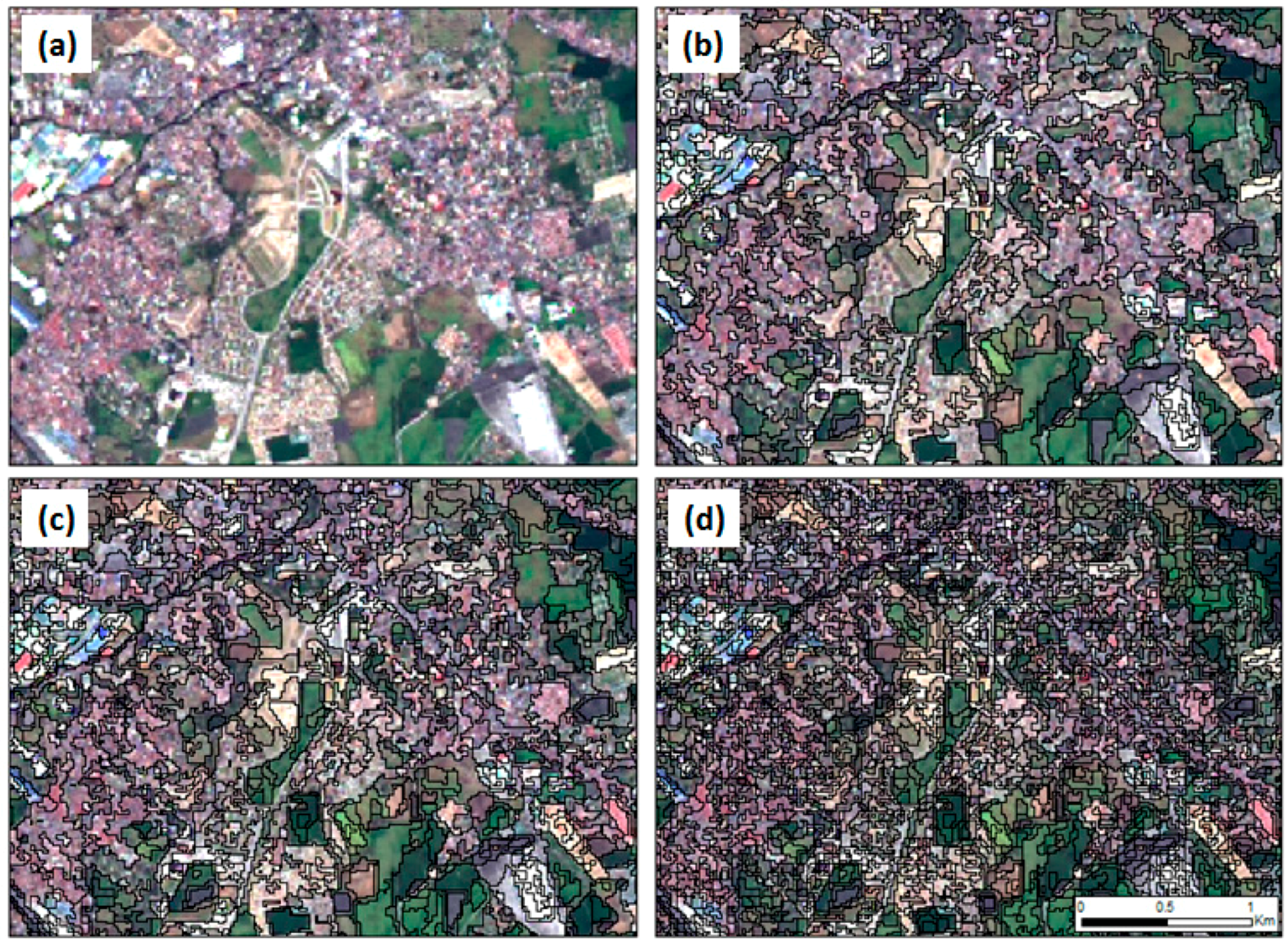
Table 1 shows the segmentations selected by USPO for SS-GEOBIA and MS-GEOBIA, and Table 2 shows the classification results for all segmentations. As can be seen in Table 2, USPO was effective for MS-GEOBIA, as the parameter-optimized MS-GEOBIA segmentations had Fclass values equal to (two-level classification) or greater than (three- and four- level classifications) that of the all-inclusive MS-GEOBIA classification, while also having fewer segmentation levels and classification variables. As an example of the multiple segmentation levels selected by USPO, Figure 3 shows the optimal segmentations selected for the three-level GEOBIA approach. In terms of residential area segmentation, the SP120 segmentation performed relatively well for segmenting large/spectrally-heterogeneous residential areas, but some smaller/more spectrally-homogeneous residential areas were undersegmented. The SP80 segmentation reduced undersegmentation of most residential areas but caused excessive oversegmentation of the larger/more heterogeneous residential areas. Finally, the SP40 segmentation caused oversegmentation of most residential areas, but was effective at detecting small vegetated patches (e.g., parks) located in residential areas.
Table 1. Optimal scale parameters (SP) for the single-scale/single-level geographic object-based image analysis (SS-GEOBIA) (one-level) and multi-scale/multi-level (MS)-GEOBIA (two-, three-, and four-level) approaches.
Number of Segmentation LevelsSP (Level 1)SP (Level 2)SP (Level 3)SP (Level 4)
180---
260100--
34080120-
44060100120
Table 2. Overall accuracy (OA), producer’s accuracy (PA), user’s accuracy (UA), and F-measure (Fclass) of the SS-GEOBIA and MS-GEOBIA approaches. Bold values show the most accurate results for each metric. The multiple SPs used for the MS-GEOBIA approaches are separated by the “+” sign.
SP(s)PA “Residential”UA “Residential”Fclass “Residential”
SS-GEOBIA200.8730.6860.768
400.8000.7210.759
600.9090.7350.813
800.8910.7210.797
1000.9270.6800.785
1200.9090.6850.781
1400.8910.7540.817
1600.9450.6930.800
1800.9090.6580.763
2000.9270.5860.718
MS-GEOBIA60 + 1000.9450.7220.819
40 + 80 + 1200.9450.7650.846
40 + 60 + 100 + 1200.9640.7460.841
All-inclusive0.9450.7220.819
USPO was also moderately effective for SS-GEOBIA, as the SP80 segmentation selected by USPO (Fclass = 0.797) outperformed more than half of the naïve segmentations. For comparison, the highest Fclass value was 0.817. The main limitation of the SS-GEOBIA parameter optimization approach for residential area mapping may have been its equal weighting of the undersegmentation and oversegmentation goodness metrics, as the residential areas were relatively larger and more spectrally-heterogeneous than the other LULC types in the study area. For this reason, in future studies, a higher weight could potentially be assigned to the oversegmentation goodness metric if the goal is only to extract the residential areas. The better performance of parameter-optimization for MS-GEOBIA was likely due to the higher weights assigned to the oversegmentation goodness metric in the coarser segmentation levels, which ensured that the residential areas were not oversegmented in at least one of the multiple segmentation levels used for classification. That being said, it is possible that other combinations of segmentation levels could lead to even higher MS-GEOBIA classification accuracies, as the number of possible combinations is very large (120 possible combinations for three-level GEOBIA in our study). It is unlikely and probably unrealistic to expect that a USPO approach will be able to always identify the best segmentation(s) to use for LULC classification, so USPO should be seen more as a way to produce generally satisfactory segmentation and classification results for SS-GEOBIA/MS-GEOBIA while requiring less time/less expert knowledge than manual trail-and-error selection of segmentation parameters. For reference, the OGf values of all segmentation levels and using all values of a are reported in Table 3.
Figure 3. (a) Subset of the study area image. Optimal segmentations for the three-level GEOBIA approach: (b) SP120 segmentation; (c) SP80 segmentation; (d) SP40 segmentation.
Ijgi 04 02292 g003
Table 3. OGf values of each segmentation level. Bold values show the segmentation level with the highest goodness for each a value (i.e., the values reported in Table 1).
One-Level GEOBIATwo-Level GEOBIAThree-Level GEOBIAFour-Level GEOBIA
SPOGf (a = 1)OGf (a = 2)OGf (a = 0.50)OGf (a = 3)OGf (a = 1)OGf (a = 0.33)OGf (a = 4)OGf (a = 2)OGf (a = 0.50)OGf (a = 0.25)
200.0000.0000.0000.0000.0000.0000.0000.0000.0000.000
400.3180.4650.2420.5500.3180.2240.5950.4650.2420.218
600.4670.5150.4270.5340.4670.4160.5420.5150.4270.411
800.4830.4510.5200.4420.4830.5340.4380.4510.5200.540
1000.4510.3850.5450.3670.4510.5860.3600.3850.5450.605
1200.3820.3000.5260.2800.3820.6030.2730.3000.5260.641
1400.3050.2260.4700.2080.3050.5740.2010.2260.4700.631
1600.2290.1610.3970.1460.2290.5260.1410.1610.3970.607
1800.1270.0840.2580.0760.1270.3920.0730.0840.2580.498
2000.0000.0000.0000.0000.0000.0000.0000.0000.0000.000

4.2. Comparison of SS-GEOBIA and MS-GEOBIA Classification Approaches
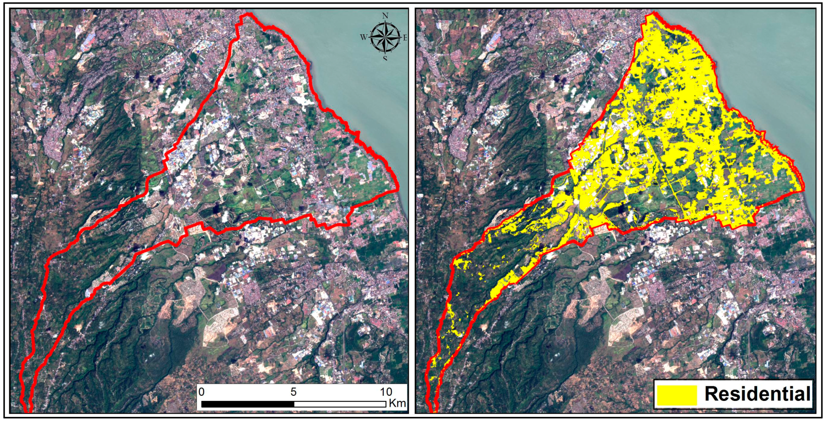
Comparing the SS-GEOBIA and MS-GEOBIA approaches, the MS-GEOBIA classifications outperformed all of the SS-GEOBIA classifications in terms of Fclass, demonstrating that multi-scale/multi-level information could improve the extraction of residential areas. Some of the finer segmentation levels (e.g., SP40) had relatively low classification accuracies when used alone for SS-GEOBIA classification, but contributed useful information for the MS-GEOBIA classifications. These findings indicate that a MS-GEOBIA classification approach can be beneficial even for mapping a single LULC type.
Figure 4. Study area image and the three-level MS-GEOBIA classification result.
Ijgi 04 02292 g004
The parameter-optimized three-level classification achieved the highest Fclass value in this study, and other studies have also suggested a three-level hierarchical approach for landscape analysis [41,42], so based on these suggestions and the results of this study, a three-level approach seems a reasonable choice for many applications. The three-level approach is also faster than an all-inclusive approach, as it requires less computation time for segmentation and spatial joining (since there are fewer segmentation levels) as well as for classification (since there are fewer classification variables). Our proposed methodology and a weights for three-level GEOBIA could thus also be useful for GEOBIA studies in other types of environments. The three-level GEOBIA classification result for the entire watershed is shown in Figure 4.

5. Conclusions

In this study, we evaluated the performance of single-scale/single-level (SS) and multi-scale/multi-level (MS) geographic object-based image analysis (GEOBIA) approaches for mapping a single land use/land cover (LULC) type; residential areas. Because manual trial-and-error selection of segmentation parameters for GEOBIA is a challenging and often time-consuming task, we also evaluated the effects of unsupervised segmentation parameter optimization (USPO) on classification accuracy, and as part of this effort we proposed a new USPO method for MS-GEOBIA which combines undersegmentation and oversegmentation “goodness” metrics using the F-measure and an adjustable weighting parameter (set based on the number of segmentation levels included for MS-GEOBIA).
We found that the MS-GEOBIA classification approaches (both “naïve” and parameter-optimized approaches) could more accurately extract residential areas than the SS-GEOBIA approach. We also found that USPO could lead to higher classification accuracy for MS-GEOBIA than a naïve (all segmentation levels inclusive) classification approach, as our parameter-optimized three-level and four-level classifications were more accurate than a naïve 10-level classification for mapping the “residential” LULC type (while the accuracy of the two-level classification matched that of the 10-level classification). The three-level classification achieved the highest classification accuracy in our study, and a three-level approach has also been recommended by other researchers for landscape analysis [41,42], so our proposed USPO approach could be particularly useful for selection of segmentation levels to include for three-level GEOBIA.
In future research, it could be useful to assess the performance of other USPO approaches for MS-GEOBIA, which are currently limited to considering either only undersegmentation goodness [42] or only oversegmentation goodness [43], for residential area mapping. It is also necessary to test the performance of our proposed MS-GEOBIA segmentation parameter optimization method for multi-class LULC classification in other urban and non-urban environments.

Acknowledgments

This paper is generally based upon outputs produced through a project on integrating climate change mitigation and adaptation, under the “Climate Change Resilient Low Carbon Society Network (CCR-LCSNet)” for the fiscal year 2014, commissioned work of the Japanese Ministry of the Environment.

Author Contributions

Brian Johnson performed the analysis and wrote the manuscript, Milben Bragais and Paula Macandog collected data and assisted with the analysis, Isao Endo, Brian Johnson, and Damasa Magcale-Macandog developed the concept for the study, and Isao Endo and Damasa Magcale-Macandog helped with drafting and revising the manuscript.

Conflicts of Interest

The authors declare no conflict of interest.

References

  1. Crowell, M.; Coulton, K.; Johnson, C.; Westcott, J.; Bellomo, D.; Edelman, S.; Hirsch, E. An estimate of the U.S. population living in 100-year coastal flood hazard areas. J. Coast. Res. 2010, 26, 201–211. [Google Scholar]
  2. Eicher, C.L.; Brewer, C.A. Dasymetric mapping and areal interpolation: Implementation and evaluation. Cartogr. Geogr. Inf. Sci. 2001, 28, 125–138. [Google Scholar] [CrossRef]
  3. Fisher, P.F.; Langford, M. Modeling sensitivity to accuracy in classified imagery: A study of areal interpolation by dasymetric mapping. Prof. Geogr. 1996, 48, 299–309. [Google Scholar] [CrossRef]
  4. Herold, M.; Scepan, J.; Clarke, K.C. The use of remote sensing and landscape metrics to describe structures and changes in urban land uses. Environ. Plan. A 2002, 34, 1443–1458. [Google Scholar] [CrossRef]
  5. Hay, G.J.; Castilla, G. Geographic object-based image analysis (GEOBIA): A new name for a new discipline. In Object-Based Image Analysis; Blaschke, T., Lang, S., Hay, G., Eds.; Springer: Heidelberg, Germany, 2008; pp. 75–89. [Google Scholar]
  6. Blaschke, T. Object based image analysis for remote sensing. ISPRS J. Photogramm. Remote Sens. 2010, 65, 2–16. [Google Scholar] [CrossRef]
  7. Herold, M.; Liu, X.; Clarke, K.C. Spatial metrics and image texture for mapping urban land use. Photogramm. Eng. Remote Sens. 2003, 69, 991–1001. [Google Scholar] [CrossRef]
  8. Kim, M.; Warner, T.A.; Madden, M.; Atkinson, D.S. Multi-scale GEOBIA with very high spatial resolution digital aerial imagery: Scale, texture and image objects. Int. J. Remote Sens. 2011, 32, 2825–2850. [Google Scholar] [CrossRef]
  9. Johnson, B.A.; Xie, Z. Classifying a high resolution image of an urban area using super-object information. ISPRS J. Photogramm. Remote Sens. 2013, 83, 40–49. [Google Scholar] [CrossRef]
  10. Waske, B.; van der Linden, S. Classifying multilevel imagery from SAR and optical sensors by decision fusion. IEEE Trans. Geosci. Remote Sens. 2008, 46, 1457–1466. [Google Scholar] [CrossRef]
  11. Johnson, B.A. High resolution urban land cover classification using a competitive multi-scale object-based approach. Remote Sens. Lett. 2013, 4, 131–140. [Google Scholar] [CrossRef]
  12. Myint, S.W.; Gober, P.; Brazel, A.; Grossman-Clarke, S.; Weng, Q. Per-pixel vs. object-based classification of urban land cover extraction using high spatial resolution imagery. Remote Sens. Environ. 2011, 115, 1145–1161. [Google Scholar] [CrossRef]
  13. Xie, Z.; Roberts, C.; Johnson, B. Object-based target search using remotely sensed data: A case study in detecting invasive exotic Australian Pine in south Florida. ISPRS J. Photogramm. Remote Sens. 2008, 63, 647–660. [Google Scholar] [CrossRef]
  14. Benz, U.C.; Hofmann, P.; Willhauck, G.; Lingenfelder, I.; Heynen, M. Multi-resolution, object-oriented fuzzy analysis of remote sensing data for GIS-ready information. ISPRS J. Photogramm. Remote Sens. 2004, 58, 239–258. [Google Scholar] [CrossRef]
  15. D’OLEIRE-Oltmanns, S.; Eisank, C.; Draguţ, L.; Blaschke, T. An object-based workflow to extract landforms at multiple scales from two distinct data types. IEEE Geosci. Remote Sens. Lett. 2013, 10, 947–951. [Google Scholar] [CrossRef]
  16. Johnson, B.A.; Tateishi, R.; Hoan, N.T. A hybrid pansharpening approach and multiscale object-based image analysis for mapping diseased pine and oak trees. Int. J. Remote Sens. 2013, 34, 6969–6982. [Google Scholar] [CrossRef]
  17. Zhang, H.; Fritts, J.E.; Goldman, S.A. Image segmentation evaluation: A survey of unsupervised methods. Comput. Vis. Image Underst. 2008, 110, 260–280. [Google Scholar] [CrossRef]
  18. Liu, D.; Xia, F. Assessing object-based classification: Advantages and limitations. Remote Sens. Lett. 2010, 1, 187–194. [Google Scholar] [CrossRef]
  19. Espindola, G.M.; Camara, G.; Reis, I.A.; Bins, L.S.; Monteiro, A.M. Parameter selection for region-growing image segmentation algorithms using spatial autocorrelation. Int. J. Remote Sens. 2006, 27, 3035–3040. [Google Scholar] [CrossRef]
  20. Johnson, B.A.; Xie, Z. Unsupervised image segmentation evaluation and refinement using a multi-scale approach. ISPRS J. Photogramm. Remote Sens. 2011, 66, 473–483. [Google Scholar] [CrossRef]
  21. Chen, J.; Deng, M.; Mei, X.; Chen, T.; Shao, Q.; Hong, L. Optimal segmentation of a high-resolution remote-sensing image guided by area and boundary. Int. J. Remote Sens. 2014, 35, 6914–6939. [Google Scholar] [CrossRef]
  22. Yue, A.; Yang, J.; Zhang, C.; Su, W.; Yun, W.; Zhu, D.; Liu, S.; Wang, Z. The optimal segmentation scale identification using multispectral WorldView-2 images. Sens. Lett. 2012, 10, 285–297. [Google Scholar] [CrossRef]
  23. Zhang, X.; Xiao, P.; Feng, X. An unsupervised evaluation method for remotely sensed imagery segmentation. IEEE Geosci. Remote Sens. Lett. 2012, 9, 156–160. [Google Scholar] [CrossRef]
  24. Fotheringham, A.; Brundson, C.; Charlton, M. Quantitative Geography: Perspectives on Spatial Analysis; SAGE Publications Ltd.: London, UK, 2000. [Google Scholar]
  25. Witten, I.H.; Frank, E.; Hall, M. Data Mining: Practical Machine Learning Tools and Techniques, 3rd ed.; Morgan Kaufmann: Burlington, MA, USA, 2011. [Google Scholar]
  26. Zhang, X.; Feng, X.; Xiao, P.; He, G.; Zhu, L. Segmentation quality evaluation using region-based precision and recall measures for remote sensing images. ISPRS J. Photogramm. Remote Sens. 2015, 102, 73–84. [Google Scholar] [CrossRef]
  27. Martha, T.R.; Kerle, N.; Westen, C.J.; van Jetten, V.; Kumar, K.V. Segment optimization and data-driven thresholding for knowledge-based landslide detection by object-based image analysis. IEEE Trans. Geosci. Remote Sens. 2011, 49, 4928–4943. [Google Scholar] [CrossRef]
  28. Ikokou, G.B.; Smit, J. A technique for optimal selection of segmentation scale parameters for object-oriented classification of urban scenes. S. Afr. J. Geomat. 2013, 2, 358–369. [Google Scholar]
  29. USGS EarthExplorer. Available online: http://earthexplorer.usgs.gov/ (accessed on 30 June 2015).
  30. Fasbender, D.; Radoux, J.; Bogaert, P. Bayesian data fusion for adaptable image pansharpening. IEEE Trans. Geosci. Remote Sens. 2008, 46, 1847–1857. [Google Scholar] [CrossRef]
  31. Johnson, B.A.; Tateishi, R.; Hoan, N.T. Satellite image pansharpening using a hybrid approach for object-based image analysis. ISPRS Int. J. Geo-Inf. 2012, 1, 228–241. [Google Scholar] [CrossRef]
  32. Baatz, M.; Schape, A. Multiresolution Segmentation—An Optimization Approach for High Quality Multi-Scale Image Segmentation. Available online: http://www.ecognition.com/sites/default/files/405_baatz_fp_12.pdf (accessed on 15 October 2015).
  33. Walker, J.S.; Blaschke, T. Object based land cover classification for the Phoenix metropolitan area: Optimization vs. transportability. Int. J. Remote Sens. 2008, 29, 2021–2040. [Google Scholar] [CrossRef]
  34. Drăguţ, L.; Tiede, D.; Levick, S.R. ESP: A tool to estimate scale parameter for multiresolution image segmentation of remotely sensed data. Int. J. Geogr. Inf. Sci. 2010, 24, 859–871. [Google Scholar] [CrossRef]
  35. Jensen, J.R. Introductory Digital Image Processing—A Remote Sensing Perspective, 3rd ed.; Pearson Prentice Hall: Upper Saddle River, NJ, USA, 2005. [Google Scholar]
  36. Sokolova, M.; Japkowicz, N.; Szpakowicz, S. Beyond accuracy, F-Score and ROC: A family of discriminant measures for performance evaluation. In AI 2006: Advances in Artificial Intelligence; Springer: Berlin, Geramny, 2006; pp. 1015–1021. [Google Scholar]
  37. Breiman, L. Random forests. Mach. Learn. 2001, 45, 5–32. [Google Scholar] [CrossRef]
  38. Lawrence, R.; Wood, S.; Sheley, R. Mapping invasive plants using hyperspectral imagery and breiman cutler classifications (RandomForest). Remote Sens. Environ. 2006, 100, 356–362. [Google Scholar] [CrossRef]
  39. Hall, M.; Frank, E.; Holmes, G.; Pfahringer, B.; Reutemann, P.; Witten, I.H. The WEKA data mining software: An update. ACM SIGKDD Explor. Newsl. 2009, 11, 10–18. [Google Scholar] [CrossRef]
  40. Bruzzone, L.; Carlin, L. A multilevel context-based system for classification of very high spatial resolution images. IEEE Trans. Geosci. Remote Sens. 2006, 44, 2587–2600. [Google Scholar] [CrossRef]
  41. Hay, G.J.; Marceau, D.J.; Bouchard, A. Modeling multi-scale landscape structure within a hierarchical scale-space framework. Int. Arch. Photogramm. Remote Sens. Spat. Inf. Sci. 2002, 34, 532–535. [Google Scholar]
  42. Drăguţ, L.; Csillik, O.; Eisank, C.; Tiede, D. Automated parameterisation for multi-scale image segmentation on multiple layers. ISPRS J. Photogramm. Remote Sens. 2014, 88, 119–127. [Google Scholar] [CrossRef] [PubMed]
  43. Meng, Y.; Lin, C.; Cui, W.; Yao, J. Scale selection based on Moran’s I for segmentation of high resolution remotely sensed images. In Proceedings of the 2014 IEEE International Geoscience and Remote Sensing Symposium (IGARRS), Quebec, QC, Canada, 13–18 July 2014; pp. 4895–4898.