Local Edge Matching for Seamless Adjacent Spatial Datasets with Sequence Alignment

Abstract

This study proposes a local edge matching method with a sequence alignment technique for adjacent spatial datasets. By assuming that the common boundary edges of the datasets are point strings, the proposed method obtains the sequence for point edit operations to align the edges by using the string matching algorithm with the following operations: (1) snapping two points from each string to their average position, (2) removing a point from one string and (3) removing a point from the other string. The costs for these operations are derived from the deformation of the involved line segments in terms of the angle and length changes. The corresponding point pairs are then considered point pairs for which the snapping operation is chosen in a sequence. Based on these pairs, a border area of adjacent spatial datasets can be partitioned into sub-border areas where distinctive matching and alignment processes can be performed.

1. Introduction

Edge matching between adjacent spatial datasets finds and removes the geometric differences of common boundary edges between adjacent spatial datasets [1,2,3,4]. There are two components in this task: feature matching to identify the corresponding point or edge pairs and map alignment to remove the differences in the identified pairs.

Because map alignment is performed with the corresponding point pairs, point feature matching is generally used in the field of geospatial information. For this reason, diverse point matching methods have been proposed. Beard and Chrisman proposed the Zipper algorithm, which finds the closest point pairs within a distance threshold and determines that these pairs are the corresponding point pairs [1]. This algorithm is simple and efficient; thus, it has been adopted in many studies [2,3,4,5]. However, one problem with this algorithm lies in estimating an appropriate threshold because even though the threshold is related to the positional accuracies of the spatial datasets involved, it is not clear how the accuracies are translated into a threshold value [6]. To address this problem, a statistical analysis of the sampled corresponding point pairs in the training data was applied. Lolonis [4] proposed a chi-square analysis on the positional differences of candidate corresponding point pairs and then discriminated mismatched pairs according to the level of statistical confidence. Masuyama [5] determined the threshold with a Monte-Carlo simulation-based analysis of the sampled pairs. Huh et al. [7] used a box-plot analysis on the sampled pairs because the analysis can discriminate proper and outlier values in the sampled pairs without any assumption of an underlying statistical distribution. Meanwhile, map alignment methods without the above feature matching were recently proposed [6,8]. They represent the geometric differences of adjacent spatial datasets as gaps and overlaps. The gaps and overlaps stand for erroneous areas where no spatial data coverage exists and where coverage from different datasets co-exists, respectively. These areas are decomposed into triangles by using computational geometry techniques such as a constrained Delaunay triangulation method. Then, each of the triangles [6] or divided parts of each of the triangles [8] is assigned to one of the spatial datasets and seamless common boundary edges without gaps and overlaps are obtained.

Although the above studies have presented successful results, additional improvements are necessary in feature matching to address locally auto-correlated positional differences. In the field of map conflation, which finds corresponding point pairs or corresponding objects between super-imposed spatial datasets, a transformation model such as an affine or rigid transformation model is applied to explain the auto-correlated positional differences. These types of differences also arise in the edge matching shown as sub-border areas in Figure 1. By considering the horizontal direction differences of the corresponding point pairs in sub-border area 1, (a₍₁₎, b₍₁₎), (a₍₂₎, b₍₂₎), (a₍₃₎, b₍₃₎) and (a₍₄₎, b₍₄₎) are proper corresponding point pairs. However, (a₍₃₎, b₍₂₎) and (a₍₅₎, b₍₄₎) are closest pairs and thus would be chosen for the corresponding point pairs when a general matching method is applied. Meanwhile, there are vertical direction differences for the corresponding point pairs in sub-border area 3. When there are many sub-border areas whose positional difference directions are distinctive, these differences cannot be explained by a single transformation model.

Moreover, this problem can be more severe when there are many road or river objects that are divided by boundaries of adjacent spatial datasets and are partially represented in each dataset. When the two datasets are constructed by the same mapping agency with the same mapping rule, divided spatial objects have the same attributes, including the name or identification code. In this case, these objects are found first and then the corresponding point pairs of each corresponding object pair can be easily found. When the two datasets are not constructed by the same mapping agency with the same mapping rule, only geometric properties such as distance or shape are available to find corresponding point pairs. However, feature matching with these geometric properties is vulnerable to the aforementioned problem in Figure 1. Moreover, this problem could not be addressed by a transformation model because the border area’s length is often more than several kilometres and a simple model cannot explain locally distinctive differences.

Figure 1. Positional differences between adjacent spatial datasets.

Figure 1. Positional differences between adjacent spatial datasets.

To address this problem, this study proposes a local edge matching method with sequence alignment by using a string matching algorithm. By assuming that the border boundary edges of two adjacent maps are point strings, the proposed method obtains the sequence for point edit operations to align the edges by using the following operations: (1) snapping two points from each string to their average position, (2) removing a point from one string and (3) removing a point from the other string. The costs for these operations are derived from the deformation of the involved line segments in terms of the angle and length changes. The optimal operation sequence with the minimum total cost is obtained by means of a dynamic programming optimization technique [9,10]. The corresponding point pairs are then considered point pairs for which the snapping operation is chosen in a sequence. Based on these pairs, a border area of adjacent spatial datasets can be partitioned into sub-border areas where distinctive matching and alignment processes can be performed.

The remainder of the paper is structured as follows. In the next section, the details of the proposed method are presented. In Section 3, the results of the proposed method are evaluated and discussed. The proposed method is applied to two cadastral maps of neighbouring local authorities. The result of the proposed method is compared with manually chosen corresponding point pairs and with a conventional distance threshold method. Finally, the conclusion is given in Section 4.

2. Proposed Method

The proposed method consists of four steps: Step 1. Extraction of point strings from adjacent spatial datasets, Step 2. String matching for extracted point strings, Step 3. Local map transformation and matching for disconnected line segments and Step 4. Local map alignment to remove gaps and overlaps as shown in Figure 2. The details for this method are as follows.

Figure 2. Workflow of the proposed method.

Figure 2. Workflow of the proposed method.

2.1. Extraction of Point Strings from Adjacent Spatial Datasets

This step is a preprocessing step to extract boundary point strings from spatial datasets. Technically, different data manipulations are necessary according to the data type of involved spatial datasets. In this study, there are two assumptions regarding spatial datasets. The first assumption is that these datasets are built and maintained by mapping agencies only for their own catchment areas, so that the boundaries of the datasets present a seamless spatial dataset after edge matching. The other assumption is that the datasets are composed of polygon objects that are mutually exclusive and collectively exhaustive, such as a cadastral map.

Currently, it is necessary to define a border area where point strings to be matched and aligned are extracted. This area is obtained as a union area of buffered boundaries for two spatial datasets (Figure 3c). With a buffer distance $Th$, each spatial dataset’s boundaries are extended (Figure 3a,b) and all line segments and points for these datasets within the union area are extracted. Then, line segments that are not for each dataset’s boundary edges are obtained as duplicate pairs because of the aforementioned assumptions (Figure 3d). These duplicate segments are removed and the remaining line segments are concatenated into polylines, which are represented as point strings (Figure 3e). Later, these removed line segments connected to these point strings are used for matching the disconnected line segments in Step 3.

Figure 3. Extraction of point strings from adjacent spatial datasets; (a) buffer zone of boundary of map A, (b) buffer zone of boundary of map B, (c) union area of buffer zones of boundaries of map A and B, (d) line segments extracted by union area, (e) point strings to be aligned.

Figure 3. Extraction of point strings from adjacent spatial datasets; (a) buffer zone of boundary of map A, (b) buffer zone of boundary of map B, (c) union area of buffer zones of boundaries of map A and B, (d) line segments extracted by union area, (e) point strings to be aligned.

It is notable to determine the order of the point strings. In general, the point order of a simple polygon is counter-clockwise. Similarly, end points for each point string are connected temporarily, and then the orders are determined to be counter-clockwise.

2.2. String Matching for Extracted Point Strings

2.2.1. Cost Function

The proposed method uses three types of point edit operations. The snapping operation $o\left(a_{\left(i\right)},b_{\left(j\right)}\to v\right)$ moves two points, one from each string, to their average position $v$, as shown in Figure 4a. The removing operation $o\left(a_{\left(i\right)}\to \varphi \right)$ or $o\left(b_{\left(j\right)}\to \varphi \right)$ removes a point of one string, as shown in Figure 4b. Because the removing operations remove the points of the boundaries, only point pairs for snapping operations remain and are used for subsequent edit operations. Thus, $p$ is the point of the average position of two points for the latest snapping operation.

Figure 4. Cost functions of string matching in this study; (a) snapping operation, (b) removing operation.

Figure 4. Cost functions of string matching in this study; (a) snapping operation, (b) removing operation.

These operations change the shapes of the boundary edges by moving or removing involved points. There have been studies to align boundaries for the corresponding object pairs with point edit operations [7,11,12,13]. These studies proposed various cost functions quantitatively to measure the change in the shape by finding the optimal point edit operation sequence with the minimum total cost. Among the cost functions, we choose the deformation energy model [7]. It measures the change in terms of the stretching and bending energy, as expressed by Equation (1).

$$E=E_{stretching}+E_{bending}=\lambda {\left(\Delta l\right)}^2+\left(1-\lambda \right){\left(\Delta \theta \right)}^2$$

(1)

Here, $\text{Δ}l$ and $\text{Δ}\theta$ are the length and angle differences caused by an operation, respectively, and $\text{λ}\left(0\le \text{λ}\le 1\right)$ is a coefficient for the weighted summarization of the stretching and bending energy.

In Figure 4a, the snapping operation $o\left(a_{\left(i\right)},b_{\left(j\right)}\to v\right)$ changes the lengths and angles of four boundary line segments. Thus, according to Equation 1, the cost of the snapping operation is determined by Equation (2).

$$\begin{array}{l}c\left(a_{(i)},b_{(j)}\to v\right)=\lambda \left\{{\left(l_{p,a(i)}-l_{p,v}\right)}^2+{\left(l_{a(i),a(i+1)}-l_{v,a(i+1)}\right)}^2+{\left(l_{p,b(j)}-l_{p,v}\right)}^2+{\left(l_{b(j),b(j+1)}-l_{v,b(j+1)}\right)}^2\right\}\\ +\left(1-\lambda \right)\left\{{{\theta }_p}^2+{{\theta }_{a(i+1)}}^2+{{\theta }_{p\text{'}}}^2+{{\theta }_{b(j+1)}}^2\right\}\end{array}$$

(2)

In this equation, $l_{x,y}$ is the length (meter) of a boundary line segment between points $x$ and $y$. ${\theta }_x$ is the angle change (degree) at point $x$ after an operation.

In Figure 4b, the removing operation $o\left(a_{\left(i\right)}\to \varphi \right)$ changes the lengths and angles of two line segments of one boundary. Thus, the cost of the removing operation is formulated as Equation (3).

$$c\left(a_{(i)}\to \varphi \right)=2\lambda \left\{{\left(\frac{l_{p,a(i)}+l_{a(i),a(i+1)}-l_{p,a(i+1)}}{2}\right)}^2\right\}+\left(1-\lambda \right)\left\{{{\theta }_p}^2+{{\theta }_{a(i+1)}}^2\right\}$$

(3)

The other removing operation $o\left(b_{\left(j\right)}\to \varphi \right)$ is similarly formulated.

2.2.2. String Matching to Find Corresponding Point Pairs

Given two point strings $A=\left[a_{\left(1\right)},a_{\left(2\right)},\cdots ,a_{\left(n\right)}\right]$ and $B=\left[b_{\left(1\right)},b_{\left(2\right)},\cdots ,b_{\left(m\right)}\right]$ whose sizes are $n$ and $m$, respectively, a string matching method calculates the total cost between $A$ and $B$, as described by Equation (4).

$$C\left(A,B\right)=\text{\hspace{0.17em}\hspace{0.17em}\hspace{0.17em}min\hspace{0.17em}}\left\{{\displaystyle \sum _O{c}_{(i)}|O=\left[o_{(1)},o_{(2)},\cdots ,o_{(N)}\right]}\right\}$$

(4)

Here, $o_{\left(i\right)}$ is one type of edit operation and $c_{\left(i\right)}$ is the cost of $o_{\left(i\right)}$. $N$ is the total number of edit operations. Given the two point strings and the cost functions, the optimal sequence $O$ is obtained by the dynamic programming technique shown in Figure 5 based on the following property of Equation (5) [14].

$$C\left(A_{<1,i>},B_{<1,j>}\right)=\text{\hspace{0.17em}\hspace{0.17em}\hspace{0.17em}min\hspace{0.17em}}\left\{\begin{array}{l}C\left(A_{<1,i-1>},B_{<1,j-1>}\right)+c\left(a_{(i)},b_{(j)}\to v|P\left(i-1,j-1\right)\right)\\ C\left(A_{<1,i-1>},B_{<1,j>}\right)+c\left(a_{(i)}\to \varphi |P\left(i-1,j\right)\right)\\ C\left(A_{<1,i>},B_{<1,j-1>}\right)+c\left(b_{(j)}\to \varphi |P\left(i,j-1\right)\right)\end{array}\right\}$$

(5)

Here, $A_{\langle 1,i\rangle }=\left[a_{\left(1\right)},a_{\left(2\right)},\cdots ,a_{\left(i\right)}\right]$ and $B_{\langle 1,j\rangle }=\left[b_{\left(1\right)},b_{\left(2\right)},\cdots ,b_{\left(j\right)}\right]$ denote two partial point strings from $a_{\left(1\right)}$ to $a_{\left(i\right)}$, and from $b_{\left(1\right)}$ to $b_{\left(j\right)}$, respectively. $\text{c}(\bullet |p)$ indicates the cost for a point edit operation whose point pair of the latest snapping operation is $p$. As explained earlier, the above cost functions need the point pairs for the latest snapping operation. To support this information when calculating $\text{C}\left(A_{\langle 1,i\rangle },B_{\langle 1,j\rangle }\right)$, matrix $P$ is constructed in Figure 5. A distance constraint for the snapping operation to improve the matching accuracy is added; the distance between the corresponding points is less than $Th$. This parameter is the same as the buffer distance in the previous step.

However, the point pairs for the snapping edit operations cannot be directly obtained from the total cost. They are obtained from an edit operation matrix $T$, where $T\left(i,j\right)$ denotes the latest chosen edit operation of $\text{C}\left(A_{\langle 1,i\rangle },B_{\langle 1,j\rangle }\right)$. From this matrix, the optimal edit sequence for $\text{C}\left(A_{\langle 1,i\rangle },B_{\langle 1,j\rangle }\right)$ can be obtained by using a backtracking analysis from $T\left(i,j\right)$. This finds the previously chosen edit operation among $\left(a_{\left(i\right)}\to \varphi \right)$ from $T\left(i-1,j\right)$, $o\left(b_{\left(j\right)}\to \varphi \right)$ from $T\left(i,j-1\right)$ and $o\left(a_{\left(i\right)},b_{\left(j\right)}\to v\right)$ from $T\left(i-1,j-1\right)$ [7]. Thus, starting from $T\left(n,m\right)$, the point edit operation sequence to $T\left(0,0\right)$ is traced and the corresponding point pairs are obtained as the pairs for which the snapping operations are chosen.

Figure 5. Pseudo code for string matching in this study.

Figure 5. Pseudo code for string matching in this study.

2.3. Local Map Transformation and Matching for Disconnected Line Segments

The point strings extracted in Step 1 are divided into sub-point strings and are locally aligned by a rigid transformation according to the average position of corresponding points as shown in Figure 6. Although the string matching in this study finds most of the corresponding point pairs between common boundaries of adjacent spatial datasets, it does not work well for points of disconnected lines segments as shown in Figure 6a. This is because the string matching in this study searches the edit sequence to align two point strings with the minimum cost. Generally, points on the disconnected line segments are incident to almost straight segments and their removing operation often causes a smaller amount of deformation compared with their snapping operation. Therefore, it often misses the corresponding point pairs of the disconnect line segments. To solve this problem, the mutually closest point pairs within a tolerance distance $tol$ are also chosen in post-processing as shown in Figure 6a. Meanwhile, there are no point pairs within $tol$ in Figure 6b,c.

Figure 6. Local map transformation of corresponding sub-point string pair; (a) two corresponding point pairs are found after transformation, (b,c) no additional corresponding point pairs are found and there remain spatial inconsistences after transformation.

Figure 6. Local map transformation of corresponding sub-point string pair; (a) two corresponding point pairs are found after transformation, (b,c) no additional corresponding point pairs are found and there remain spatial inconsistences after transformation.

2.4. Map Alignment to Remove Gap and Overlap

After the above map transformation, there are three types of geometric differences: linear difference (Figure 7a), triangle difference (Figure 7b) and polygonal difference (Figure 7c). The linear difference is a case when every point for the sub-point strings has its own corresponding points so that snapping these point pairs to their average positions removes their geometric differences. The triangle difference is a case when one sub-point string is a line segment and the other is a polyline with two line segments. In this case, an aligned boundary edge is obtained by connecting the snapped corresponding points via the centroid of the triangle.

Figure 7. Map alignment method for geometric difference case in this study; (a) linear difference, (b) triangle difference and (c) polygon difference.

Figure 7. Map alignment method for geometric difference case in this study; (a) linear difference, (b) triangle difference and (c) polygon difference.

The polygon difference is a complicated problem compared with the above two cases. In shape analysis, this difference is studied as a skeleton problem that finds a thin version of a shape that is equidistant to its boundaries. Among skeleton methods, a constrained Delaunay triangulation (CDT) method is applied to obtain an aligned boundary edge. CDT is a generalization of the Delaunay triangulation that forces certain line segments into the edges of triangulation. In this study, the aforementioned constraint is imposed on the line segments of the transformed boundary edge. Then, an aligned boundary edge is obtained by connecting snapped corresponding points via the mid-points of two internal edges of each triangle. The details for this CDT are explained in [15].

Sometimes, transformed corresponding sub-point strings intersect as shown in Figure 8. In this case, these strings are divided according to the intersection points and the above map alignment method is applied for each section by assuming that these intersection points are snapped corresponding points.

Figure 8. Polygon difference with intersection points of a transformed sub-point string pair.

Figure 8. Polygon difference with intersection points of a transformed sub-point string pair.

3. Experiment and Discussion

3.1. Dataset and Parameter Determination

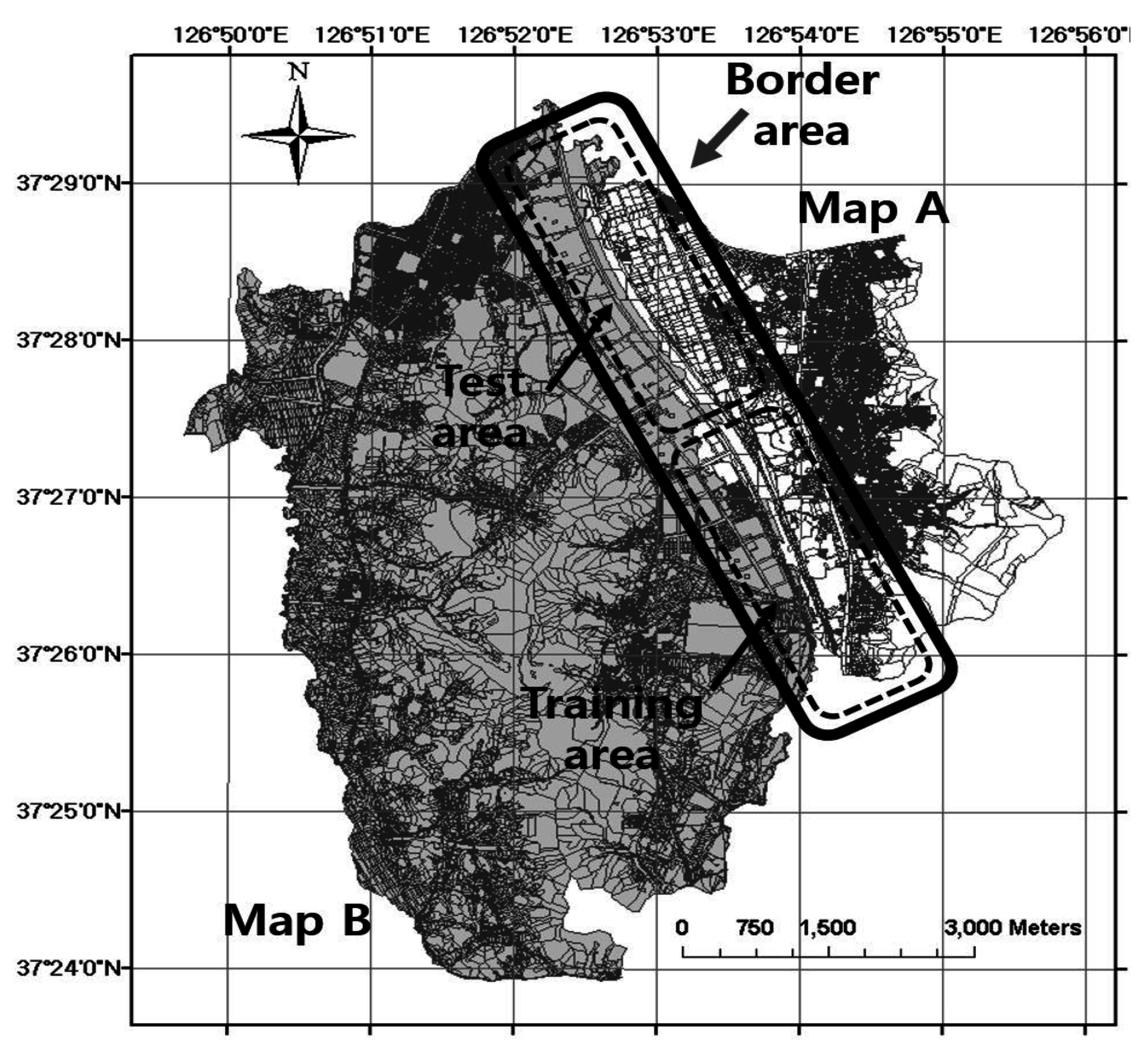
We applied the proposed method to two adjacent cadastral maps, as shown in Figure 9. Map A is a cadastral map of the Geum-Cheon district in Seoul city, and map B is a cadastral map of the Gwang-Myeong city in the Gyeong-gi province. The length of the border area is approximately 10 km. Because these maps are created by joining the respective legacy parcel maps and they are maintained independently by local authorities, irregular positional discrepancies arise between the boundary edges of the maps.

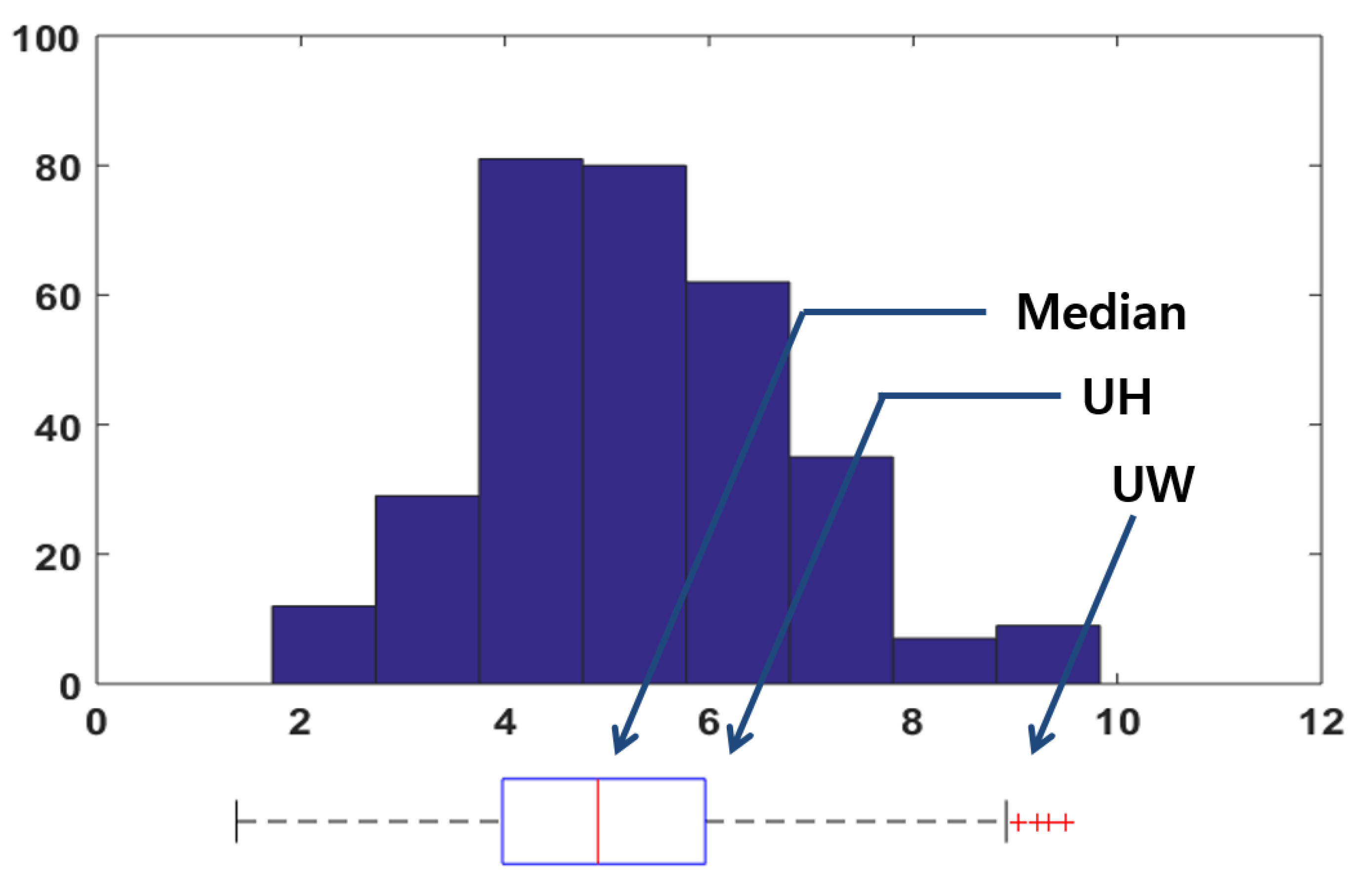
The proposed method has three parameters: $Th$, $\lambda$ and $tol$. Among them, $Th$ is determined by a statistical analysis of 351 corresponding point pairs in the training area of Figure 9. We apply the boxplot method [16] to determine $Th$ because the threshold should be a feasible upper limit of the lengths for the corresponding point pairs. The method begins by finding the median of the training data and then doing the same for each of the halves. These upper and lower quartiles define the centre box and are often referred to as the upper hinge ($UH$) and lower hinge ($LH$), respectively. The upper inner fence ($UIF$) is defined as an upper fence of the box that is extended by 1.5 times the length of the box towards the maximum, and the upper whisker ($UW$) is defined as the farthest observation inside the $UIF$, as expressed by Equations (6) and (7), respectively, and as used for $Th$. $UW$ is used for $Th$, and it has a value of 8.89 m as calculated from the pairs in the training data, as shown in Figure 10.

$$UIF=UH+1.5\cdot \left(UH-LH\right)$$

(6)

$$UW=\text{\hspace{0.17em}\hspace{0.17em}\hspace{0.17em}max\hspace{0.17em}}\left(x|x<UIF\right)$$

(7)

Figure 9. Two adjacent cadastral maps (map A and map B) for the experiments.

Figure 9. Two adjacent cadastral maps (map A and map B) for the experiments.

Figure 10. A histogram and boxplot analysis of manually chosen corresponding point pairs.

Figure 10. A histogram and boxplot analysis of manually chosen corresponding point pairs.

Meanwhile, the remaining parameters $\lambda$ and $tol$ cannot be directly trained by this analysis. Thus, various values of the parameters are evaluated and then the optimal parameters with the highest level of matching accuracy are obtained. We used three types of measures for the accuracy: precision, recall and the F-measure. Precision refers to the ratio of correctly found pairs over the total number of found pairs and recall denotes the ratio of correctly found pairs to the total number of correct pairs. The F-measure is defined by Equation (8). In this equation, $P$ and $R$ represent precision and recall, respectively.

$$F-Measure=\frac{2\cdot P\cdot R}{P+R}$$

(8)

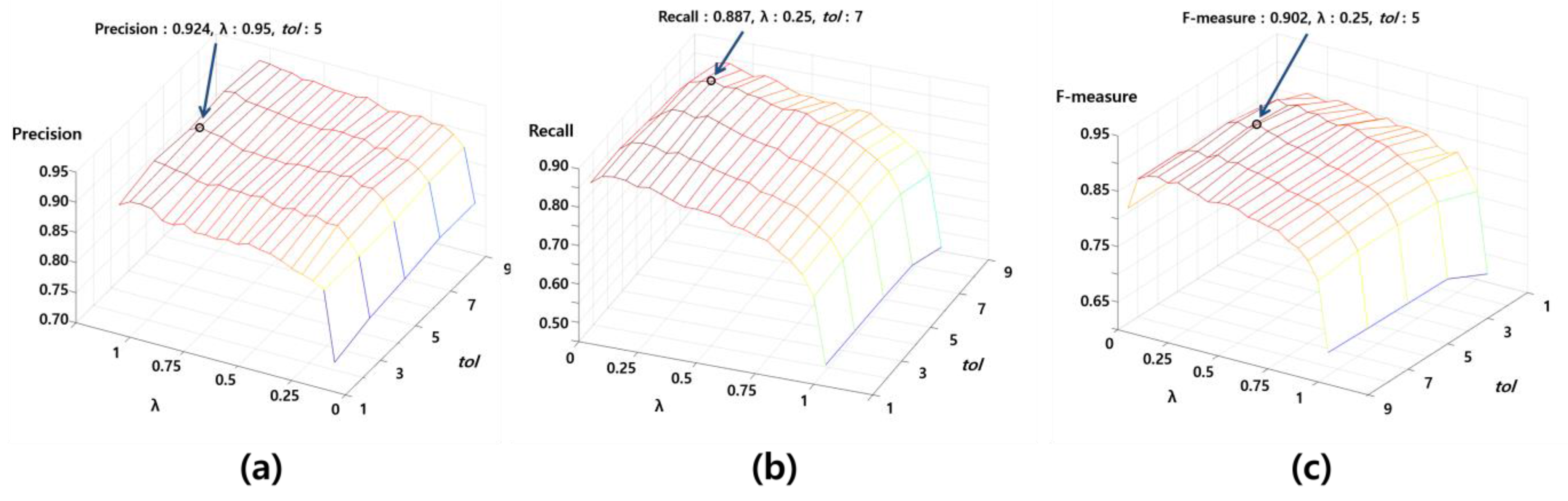
We applied 21 candidate $\lambda$s from 0 to 1 with 0.05 intervals and five candidate $tol$s from 1 m to 9 m with 2 m intervals. The highest precision (0.924) was obtained when $\lambda$ and $tol$ were 0.95 and 5 m, respectively, as shown in Figure 11a. In addition, the highest recall (0.887) was obtained when $\lambda$ and $tol$ were 0.25 and 7 m, respectively, as shown in Figure 11b. According to $\lambda$, precision and recall presented a trade-off relationship. When $\lambda$ increased and became closer to one, the degree of precision increased. Meanwhile, when $\lambda$ decreased and became closer to zero, the degree of recall increased. Thus, $\lambda$ serves as a matching threshold for the proposed method. In general, a tighter threshold presents a smaller number of matching pairs with higher precision and lower recall, whereas a looser threshold presents a larger number of matching pairs with lower precision and higher recall. In this study, the proposed method uses the snapping and removing edit operations. In addition, one of the operations that presents the minimum total cost is chosen for a given point. Accordingly, a matching result with high precision and low recall according to a large $\lambda$ indicates an increase in the cost of the snapping operation. Meanwhile, a matching result with low precision and high recall according to a small $\lambda$ indicates a decrease in the cost of the snapping operation. Compared with $\lambda$, $tol$ does not have a meaningful effect on the matching performance. As a result, the highest F-measure (0.902) was obtained when $\lambda$ and $tol$ were 0.25 and 5 m, respectively, as shown in Figure 11c.

Figure 11. Accuracy evaluations of the proposed method according to the two parameters $\lambda$ and $tol$: (a) precision, (b) recall and (c) the F-measure.

Figure 11. Accuracy evaluations of the proposed method according to the two parameters $\lambda$ and $tol$: (a) precision, (b) recall and (c) the F-measure.

3.2. Result and Discussion

To compare the performance and find the corresponding point pairs for edge matching, a statistical evaluation of the proposed method and a distance threshold method is performed in the test area. As shown in Table 1, precision, recall and F-measure values of the distance threshold method with Th of 8.89 m were 0.761, 0.927 and 0.835, respectively. Meanwhile, the proposed method with the parameters determined in the previous section showed higher precision and F-measure values; however, they also showed a lower recall value. These findings indicate that the proposed method has a tighter matching criterion and that the overall matching result of the proposed method was better than that of the conventional distance threshold method in terms of the F-measures.

Table 1. The statistical evaluation of the proposed method and a distance threshold method in the test area in Figure 9.

	The Proposed Method with Th: 8.89 m, λ:0.25 and tol: 5 m	A Distance Threshold Method with Th: 8.89 m
Precision	0.912	0.761
Recall	0.895	0.927
F-measure	0.903	0.835

Table 1. The statistical evaluation of the proposed method and a distance threshold method in the test area in Figure 9.

	The Proposed Method with Th: 8.89 m, λ:0.25 and tol: 5 m	A Distance Threshold Method with Th: 8.89 m
Precision	0.912	0.761
Recall	0.895	0.927
F-measure	0.903	0.835

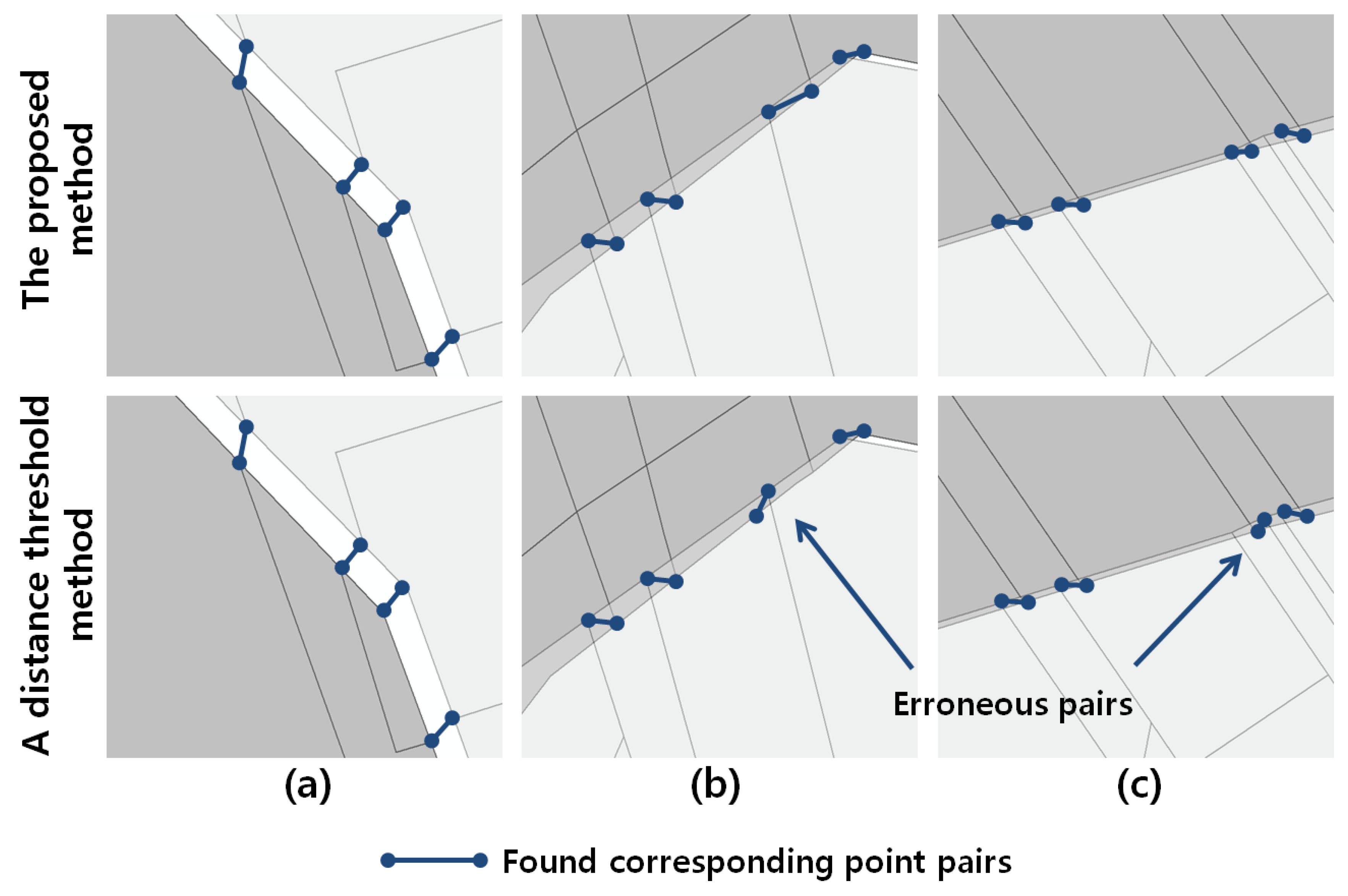
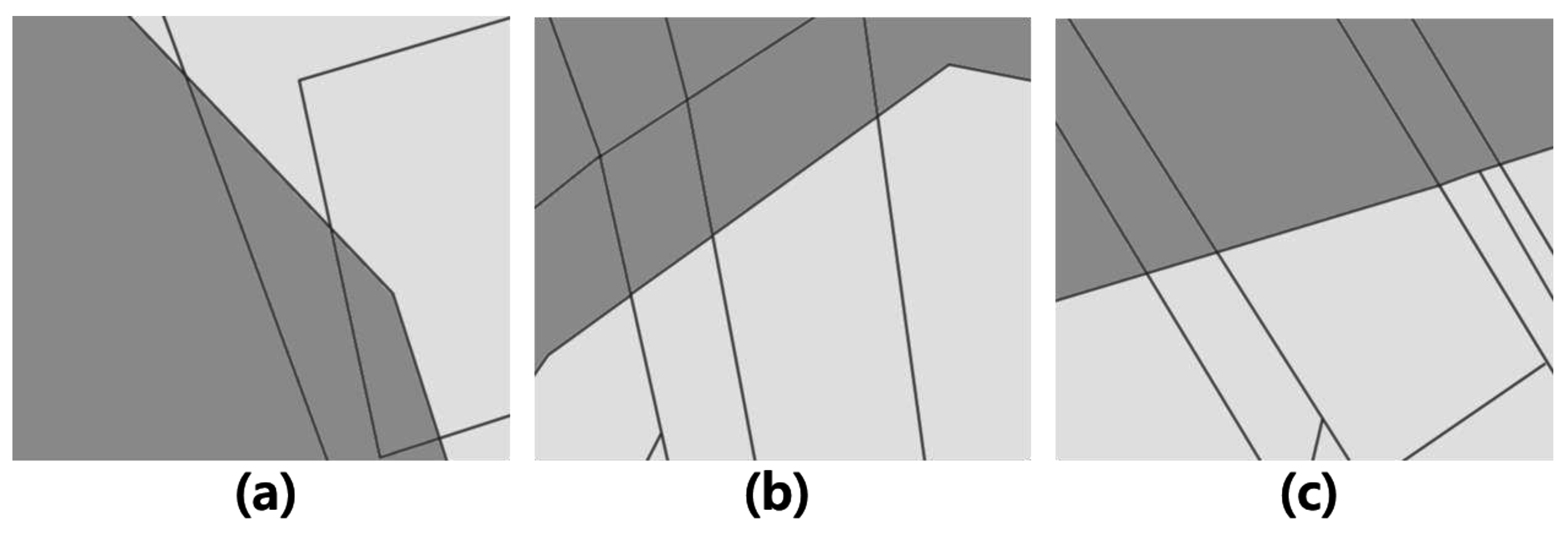
A higher precision for the proposed method was obtained especially from points on disconnected line segments, as shown in Figure 12b,c. When the distances between these points are sufficient compared with the positional discrepancies between adjacent maps, as shown in Figure 12a, the two methods presented nearly the same results. However, the distances for the erroneous point pairs are coincidently shorter than those of true point pairs, as shown in Figure 12b, which shows that the distance threshold method was vulnerable to this problem and presented an inaccurate result with low precision. This problem became even more severe for the points on parallel disconnected line segments, which describe the roads as shown in Figure 12c. Occasionally, the widths of these roads are not sufficient compared with the positional discrepancies between the maps. Therefore, many erroneous point pairs can be obtained by the distance threshold method because the closest points are simply chosen for the pairs regardless of the neighbouring auto-correlated positional discrepancies. Meanwhile, the proposed method performs a matching process by considering these discrepancies; hence, it presents an improved matching performance in terms of precision. Figure 13 is the result of map alignment with these corresponding point pairs.

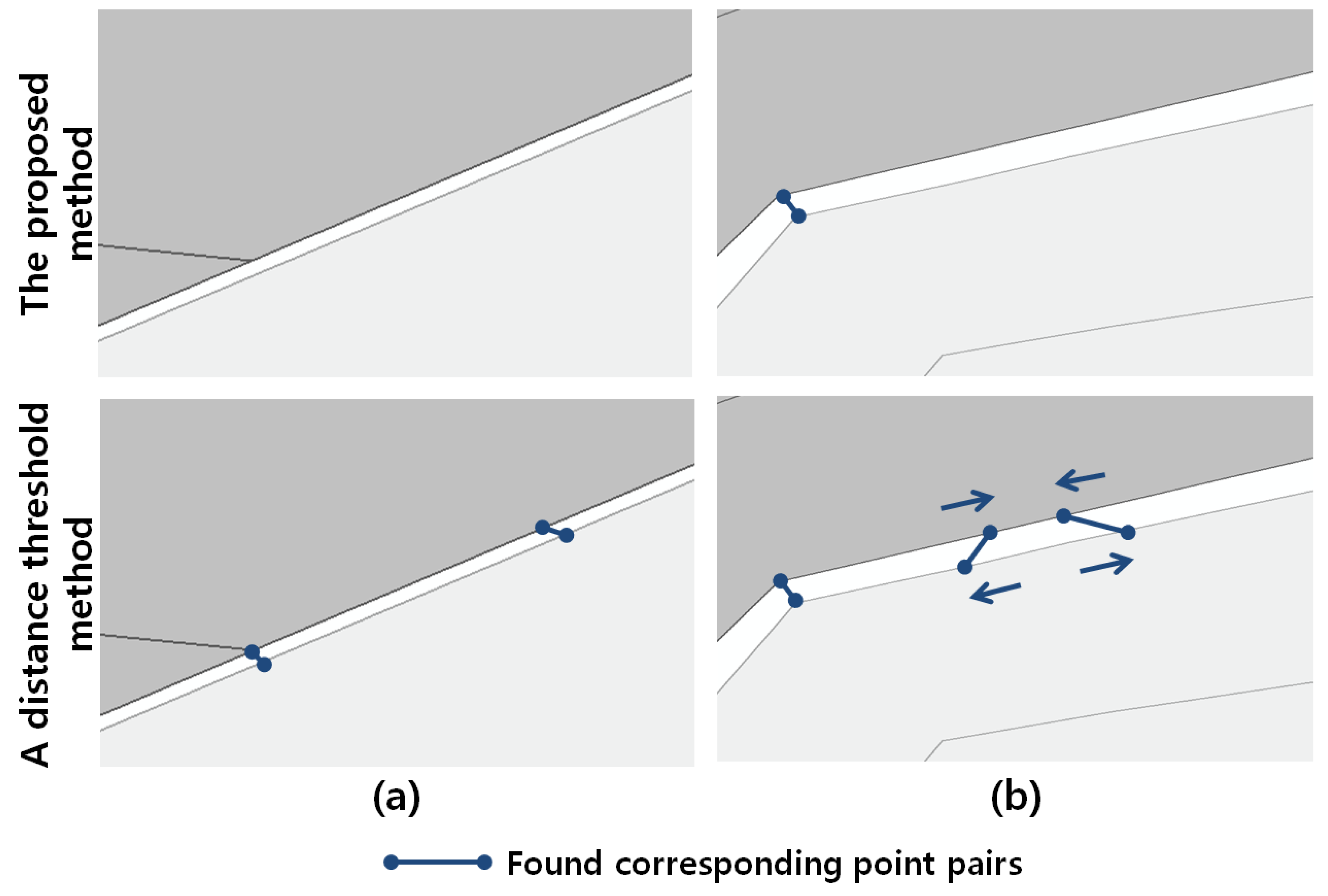
Compared with the higher degree of precision, the proposed method presented lower recall, as shown in Table 1. This occurred because it tends to choose corresponding point pairs between salient corner points rather than those on nearly straight line segments, as shown in Figure 14a. The proposed method determines corresponding point pairs as the point pairs for which the snapping operation is chosen in the optimal sequence with which two point strings are aligned at the minimum total cost. In general, the removing operation of a salient corner point causes a considerable amount of shape deformation on the line segments involved, which results in a larger edit operation cost than that of the snapping operation. This relationship is opposite for the points connected by nearly straight line segments. Thus, as shown in the previous figures, the proposed method accurately found the corresponding point pairs between salient corner areas with a higher degree of recall accuracy. However, except for those disconnected line segments, the corresponding point pairs between points connected by nearly straight line segments were not sufficiently found because the choices in removing operations for them present a lower cost. This property prevents irregular stretching or shrinking of the neighbouring border areas, as shown in Figure 14b. The proposed method found the corresponding point pairs between salient corner areas by allowing gradual map alignments along the border area to be obtained. However, when all of the mutually closest points are used, the map alignment result by itself could be abrupt, which decreases the overall performance. Based on the above comparisons to the manually chosen corresponding point pairs and the matching property, the proposed method is superior to previous distance threshold methods.

Figure 12. Comparison of corresponding point pairs found by the proposed method and the distance threshold method; (a) both methods find correct pairs, (b,c) the proposed method finds correct pairs of disconnected line segments between two maps meanwhile the distance threshold methods finds erroneous pairs.

Figure 12. Comparison of corresponding point pairs found by the proposed method and the distance threshold method; (a) both methods find correct pairs, (b,c) the proposed method finds correct pairs of disconnected line segments between two maps meanwhile the distance threshold methods finds erroneous pairs.

Figure 13. Map alignment to remove gap and overlap of Figure 12; (a) alignment result of Figure 12a, (b) alignment result of Figure 12b, (c) alignment result of Figure 12c.

Figure 13. Map alignment to remove gap and overlap of Figure 12; (a) alignment result of Figure 12a, (b) alignment result of Figure 12b, (c) alignment result of Figure 12c.

Additionally, it is necessary to discuss the effect of point string order. In Section 2.1, the orders were determined to be counter-clockwise. However, according to the order of whether it is counter-clockwise or clockwise, matching results for the corresponding point pairs can be different. Although both results are nearly the same, this cannot be explained at this stage and further research is necessary.

Figure 14. Comparison of corresponding point pairs found by the proposed method and the distance threshold method for straight line segments; (a) the proposed method does not find corresponding point pairs between points on nearly straight line segments meanwhile the distance threshold method finds correct pairs, (b) the distance threshold method finds corresponding point pairs which result irregular stretching or shrinking after map alignment meanwhile the proposed method does not cause such problem.

Figure 14. Comparison of corresponding point pairs found by the proposed method and the distance threshold method for straight line segments; (a) the proposed method does not find corresponding point pairs between points on nearly straight line segments meanwhile the distance threshold method finds correct pairs, (b) the distance threshold method finds corresponding point pairs which result irregular stretching or shrinking after map alignment meanwhile the proposed method does not cause such problem.

4. Conclusions

This paper proposed a new method to find corresponding point pairs for common boundary edge matching between adjacent spatial datasets by using a string matching technique with three types of point edit operations. These three operations snapped two points of the strings to their average position, removed a point of one string, and removed a point of the other string. Unlike previous distance threshold methods, the proposed method can consider local auto-correlated positional discrepancies because the choice in edit operation changes the geometries of the boundary line segments involved, after which the changed geometries affect the remaining points’ edit costs. Thus, the proposed method presented an improved matching performance compared with a previous method especially for the precision measure. This demonstrates that the proposed method finds more robust corresponding point pairs. However, it found fewer pairs from true corresponding point pairs than the previous method because according to the proposed cost functions, the costs of removing points connected by nearly straight line segments are generally lower than the costs of snapping the points. For this reason, the proposed method tends to find corresponding pairs between salient corner points and not between points connected by nearly straight line segments. However, this property results in gradual map alignments along the border area by preventing the irregular stretching or shrinking of neighbouring borders. As a result, the proposed local edge matching method showed an improved ability to find corresponding point pairs for seamless adjacent spatial datasets.

References

1. Beard, M.; Chrisman, N. Zipper: A localized approach to edge matching. Am. Cartogr. 1988, 15, 163–172. [Google Scholar] [CrossRef]
2. Coren, I.; Doytsher, Y. Cartographic edge matching: Mapping the problem towards a computer based solution. In Proceedings of the 1998 ACSM annual convention, Baltimore, MD, USA, 28 February–5 March 1998.
3. Gregory, I.; Ell, P. Error sensitive historical GIS: Identifying areal interpolation errors in timeseries data. Int. J. Geogr. Inf. Sci. 2006, 20, 135–152. [Google Scholar] [CrossRef]
4. Lolonis, P. A Chi-square statistic for checking satisfactory edge matching of maps and diagrams that depict adjacent areas. In Proceedings of FIG XXII International Congress, Washington, DC, USA, 19–26 April 2002.
5. Masuyama, A. Methods for detecting apparent differences between spatial tessellations at different time points. Int. J. Geogr. Inf. Sci. 2006, 20, 633–648. [Google Scholar] [CrossRef]
6. Ledoux, H.; Ohori, K. Edge-matching polygons with a constrained triangulation. In Proceedings of Symposium GIS Ostrava 2011, Ostrava, Czech, 24–26 January 2011; pp. 377–390.
7. Huh, Y.; Yu, K.; Heo, J. Detecting conjugate-point pairs for map alignment between two polygon datasets. Environ. Urban Syst. 2011, 35, 250–262. [Google Scholar] [CrossRef]
8. Cho, S; Punithan, M.; Gim, J.; Huh, Y. Tagging-the-triangle algorithm for partitioning features with inconsistent boundaries. Int. J. Geogr. Inf. Sci. 2014, 28, 2533–2550. [Google Scholar]
9. Kruskal, J.B. An overview of sequence comparison: Time warps, string edits, and macromolecules. SIAM Rev. 1983, 25, 201–237. [Google Scholar] [CrossRef]
10. Kaygin, S.; Bulut, M. Shape recognition using attributed string matching with polygon vertices as the primitives. Pattern Recognit. Lett. 2002, 23, 287–294. [Google Scholar] [CrossRef]
11. Maître, H.; Wu, Y. Improving dynamic programming to solve image registration. Pattern Recognit. 1987, 20, 443–462. [Google Scholar] [CrossRef]
12. Wang, C.; Stefanidis, A.; Croitoru, A.; Agouris, P. Map registration of image sequences using linear feature. Photogramm. Engin. Remote Sens. 2008, 74, 25–38. [Google Scholar] [CrossRef]
13. Huh, Y.; Yang, S.; Ga, C.; Yu, K.; Shi, W. Line segment confidence region-based string matching method for map conflation. ISPRS J. Photogramm. Remote Sens. 2013, 78, 69–84. [Google Scholar] [CrossRef]
14. Bunke, H.; Buhler, U. Applications of approximate string matching to 2D shape recognition. Pattern Recognit. 1993, 26, 1797–1812. [Google Scholar] [CrossRef]
15. Zou, J.J.; Chang, H.H.; Yan, H. Shape skeletonization by identifying discrete local symmetries. Pattern Recognit. 2001, 34, 1895–1905. [Google Scholar] [CrossRef]
16. Reimann, C.; Filzmoser, P.; Garrett, R.G. Background and threshold: Critical comparison of methods of determination. Sci. Total Environ. 2005, 345, 1–16. [Google Scholar] [CrossRef] [PubMed]