1. Introduction
The Web Map Service standard (WMS, [
1]), published by the Open Geospatial Consortium and standardized by ISO as ISO19128:2005 [
2], has been one of the most successful standards enabling the interoperability of geographic information. It allows clients to request georeferenced map images representing a wide variety of data sources, together with accompanying metadata. The standard is implemented in a wide range of open-source and commercial software, including GeoServer, MapServer, ArcGIS Server, Cadcorp SIS and ncWMS [
3] (see
http://www.opengeospatial.org/resource/products/compliant for a list of certified compliant software). An overview of the standard can be found in
Section 5.1 below. WMS is used as the visualization standard in many spatial data infrastructures such as INSPIRE [
4] and the Global Earth Observation System of Systems (GEOSS) [
5].
A common concern with Spatial Data Infrastructures (SDIs) in general, is that the user is frequently not provided with information regarding the quality of the underlying data. This is particularly important in the field of scientific data, in which the user often wishes to know about the uncertainty of the data. Although a number of methods are in use for visualizing uncertain data (such as those suggested by the INTAMAP project for visualizing uncertainty of interpolated maps [
6], some examples for mapping uncertainty of weather ensemble data [
7,
8] and several others described in [
9]) these are mostly not supported by WMS implementations, or are not supported in a standardized, consistent fashion; furthermore the relevant symbology standards (e.g., Symbology Encoding (SE), [
10]) do not provide the required flexibility to accommodate these more complex visualization types, particularly for raster data. Some solutions for using WMS and SE in uncertainty visualization for vector data are given in [
11], which focuses on use cases in spatial planning.
In this paper we describe a new profile of WMS for data quality (WMS-Q), which provides a number of mechanisms for using WMS to communicate data quality at a number of levels, from the dataset level to the level of individual samples (pixels). WMS-Q is entirely compatible with the current version of the WMS standard (1.3.0) and considers a number of underlying data types (including continuous and categorical data).
Section 2 introduces the concept of “data quality”,
Section 3 clarifies the terminology we will use in the paper,
Section 4 explores current means of representing data quality,
Section 5 describes the design of WMS-Q,
Section 6 briefly describes some current implementations of the profile,
Section 7 describes how WMS-Q has been integrated into a “quality-aware” SDI, and finally
Section 8 identifies areas of future work.
2. What is “Data Quality”?
Data quality is a concept that is difficult to define precisely. It means different things to different communities and it is sometimes confused with the amount of information. It is defined by the ISO 8402:1994 [
12] standard as the “totality of characteristics of a product that bear on its ability to satisfy stated or implied needs”. In the geospatial domain, it includes many measures including spatial accuracy, temporal accuracy, consistency, completeness, scope and attribute accuracy. There is a general consensus that quality is a
subjective concept and each user defines a dataset as having good quality when it fulfils his expectations, that is, it
fits his purpose. Unfortunately, data producers cannot anticipate the expectations of all future users. Thus, in practice they try to quantify some aspects by comparing the dataset with other reference sources that are accepted to be correct and provide a numeric quantification of the discrepancies in terms of uncertainty metrics and error statistics. Alternatively, they create a specification for their product, and for each dataset, they provide a confirmation of the product specifications conformity [
13]. When these approaches are applied to the data, a quality indicator [
14] is generated and attached to the metadata.
Data quality can be applied to different components of the data: spatial (e.g., positional accuracy), temporal (temporal accuracy), thematic (e.g., completeness, thematic accuracy, classification correctness,
etc.) [
14,
15,
16]. Some aspects covered by this paper apply to all of the above but the focus is on thematic accuracy.
3. Terminology Used in This Paper
Different communities use different terms to represent similar concepts, or the same term for different concepts. The WMS-Q profile can be applied in many different communities, including Earth Observation, climate science, meteorology, oceanography, terrestrial studies and more. Therefore we must carefully define the terms we use in this paper, which may be different from common usage in particular communities:
Dataset: The term
dataset is used in its most general sense of “a logical collection of data”. The information in a dataset may be recorded physically in a single file or a set of files and may represent a single snapshot in time, or time-evolving information. The choice of how to group data into datasets is highly community-specific; typically, data providers will decide how to group information into logical units that make sense to them and their users. Discovery metadata [
17,
18] is typically generated at the dataset level.
Variable: A variable is a measured quantity, such as temperature, velocity or a land use classification. It can be observed or calculated. In this paper we use “variable” to represent the concept; the values and their uncertainty are recorded in fields (see below).
Sample: A sample is an individual measurement or observation of a single variable. A pixel in an Earth Observation image, or a grid cell in the results of a numerical simulation, may contain several samples, one for each variable that is recorded in that pixel or cell.
Component: If the values of a variable within a dataset are uncertain, then each sample of this variable comprises more than one piece of information (for example, components could be the “most likely” value of the variable and the upper and lower confidence range representing its uncertainty). Each piece of information is known as a
component. Different ways of expressing uncertainty are described in
Section 4.3 below.
Field: A field is a collection of values of a single component. Typically this will be recorded in a data file as a multidimensional array of scalar (numeric) values.
We illustrate these concepts through two examples.
Example 1: The Sea Surface Temperature
dataset from the European Space Agency’s Climate Change Initiative (CCI-SST, [
19]) provides measurements of two
variables: sea surface temperature and sea ice area fraction, recorded on a global grid at 1/20 degree (~5 km) resolution. The
sample measurements of both variables are uncertain and therefore the values of each variable are expressed as two
components, one representing the mean value and one representing its variance. The dataset therefore contains four scalar
fields (two for each variable).
Example 2: The Landcover Classification of Landsat Barcelona-Girona scenes [
20]
dataset provides information on the land cover of that region of Catalonia, derived from satellite imagery. Each
sample (
i.e., pixel) within the dataset contains the best estimate of the land cover type (expressed as a classification code), some alternative classification values plus several measures of confidence that the classification is correct. The dataset therefore contains one
variable (land cover type) expressed as a number of scalar
fields: some categorical (classifications) and some continuous (confidence measures).
5. Design of WMS-Q
5.1. Overview of WMS
We briefly describe here the main relevant features of the WMS standard (version 1.3.0), in order to aid understanding of the WMS-Q extensions we describe in the sections below.
The data provided by a WMS server are divided into Layers, which represent the basic units of information. The server provides metadata about these Layers through a machine-readable service metadata document (also called the “Capabilities” document) that can be requested by clients through the GetCapabilities operation. All Layers have a human-readable Title field. Further metadata can be provided through external documents (both human-readable and machine-readable), which are linked to Layers in the service metadata document through the MetadataURL tag.
Georeferenced images (maps) of the Layers are requested through the
GetMap operation. There are two ways of controlling the appearance of a map image. The simplest method is for the server to advertise fixed
Styles, each of which is identified by a name that can be requested in the
GetMap request. A more sophisticated method can be provided using a WMS server that is enabled with the
Styled Layer Descriptor (SLD) [
33] extension. In this case, the client has much closer control over the appearance of the requested map image by sending the server an XML document encoded using the
Symbology Encoding (SE) standard. Such a server is often referred to as an
SLD/SE-enabled WMS server.
The WMS standard permits Layers to be arbitrarily nested within a service metadata document. Layers that have a <Name> property are
displayable (which means that they can be requested in a GetMap operation). WMS permits any Layer to be displayable, even if that Layer contains child Layers. Layers that are not displayable do not have a <Name> and are usually used as a grouping mechanism for child Layers. A WMS service metadata document therefore contains a hierarchy of Layers. The WMS standard specifies rules (Table 7 in [
1]) that govern the inheritance of properties of parent Layers by child Layers; these rules are important to the design of WMS-Q: see
Section 5.6.
The GetFeatureInfo operation allows a WMS client to retrieve more information about a specified pixel in a map image. The WMS standard does not specify a particular format for the information that is returned by the server and so implementations can differ widely in their behaviour.
5.2. Design Goals for WMS-Q
The design goals of the WMS-Q profile were:
To maintain compatibility with version 1.3.0 of the WMS standard. In other words, WMS-Q aims to be a profile of WMS, not an extension. Therefore, instead of adding new functionalities, it provides a set of rules on how to use the existing mechanisms permitted by the WMS standard to convey dataset, sample and variable level quality. In this way, standard WMS clients will be able to read information from a WMS-Q.
To re-use existing general methods for expressing data quality, where appropriate (e.g., UncertML, see
Section 4.3 above), but to avoid methods that are highly specific to particular communities.
To be independent of any particular format or convention for data or metadata storage.
To focus on conveying the thematic accuracy of both categorical and continuous raster data (including its uncertainty), but allow techniques to be more widely applicable in future (e.g., to vector data).
5.3. Identification of Conformance to WMS-Q
In WMS 1.3 and previous versions, there is no standard mechanism at present for advertising to clients that a WMS service instance conforms to a particular profile. In WMS-Q we use a Keyword at the top level of the service metadata document, with the value “WMS-Q” in the vocabulary “
http://www.geoviqua.org/def/doc/conventions/vocabulary”. Sample Capabilities documents illustrating this are referenced in
Section 5.6.
5.4. Dataset-Level Quality
In WMS-Q, datasets (see “Terminology”, above) are represented by Layers that are not displayable, but act as containers for child layers representing variables. These Layers can be arbitrarily nested within other non-displayable ones, as chosen by the data provider, to impose a logical structure. (In this case the non-displayable Layers act as “folders” and typically appear as such in the legend or the layer list in WMS client software.)
Data quality is expressed at the Dataset level by associating the relevant Layer with a MetadataURL that points to a suitable, standardized metadata document (e.g., an ISO19115 dataset descriptor). However, we recommend that data quality information be associated more precisely at the Variable level where possible.
5.5. Variable-Level Quality
In WMS-Q, Variables are represented by Layers that are immediate children of Layers that represent Datasets. Quality information at this level is provided, as with Dataset-level information, by external documents linked through MetadataURL tags. The linked ISO19115 data metadata documents will have one or more DQ_DataQuality elements reporting overall quality indicators represented by estimators or statistical summaries (e.g. root-mean-square errors or confusion matrices). Since a ISO19115 document can be used to convey several DQ_DataQuality elements, it is important to keep a link of each DQ_DataQuality to the original WMS-Q layer. This can be achieved using the sub-elements of the MD_Scope, and document level = “layer” and levelDescription = layer name. Then a linkage of a MD_Distribution can be used to describe the link to the WMS service as a whole.
If the Variable does not contain sample-level quality information, then the Layer representing the Variable will be displayable and therefore the client can request map images of the Variable. If the Variable does contain sample-level quality information, its corresponding Layer must be non-displayable, acting only as a container for child Layers that represent the
components of the samples, as will explained in the next section. This Layer contains the Keyword “qualityCollection” from the “
http://qualityml.geoviqua.org/1.0/” vocabulary. It may also contain Keywords from other vocabularies—for example, if the uncertainty of the Variable at the sample level is expressed using a set of summary statistics (see
Section 4.3 above), the Layer may be tagged with the Keyword “statisticsCollection” from the UncertML vocabulary.
5.6. Sample-Level Quality
If the Variable contains sample-level quality information all sample components of a Variable are represented as direct children of the Variable’s Layer (at the bottom level of the hierarchy, i.e., each component is a leaf node in the tree of Layers). These child Layers are displayable and are given Keyword tags that describe the semantics of the component, using terms from vocabularies such as QualityML or UncertML where possible.
Although sometimes it is convenient to visualize these components (child Layers) individually, it is often highly desirable for a WMS client to be able to display a single map image that represents the variable as whole, perhaps by overlaying contours of some uncertainty metric (e.g., variance) over a raster image representing the mean field (see
Figure 1). In some cases, this effect can be achieved by requesting separate images from the server (one for each component) and composing them on the client. However, this method does not work for some methods of visualizing data quality (for example, bivariate colour maps, see below). For this reason, WMS-Q servers provide an extra displayable Layer as a sibling of the other child Layers that represent components. This “special” child Layer represents the Variable as a whole and is given the Keyword “qualityComposition”. It is the first Layer to be listed as a direct child of the Layer representing the Variable (in this case it can also have a metadata document describing its quality attached in the MetadataURL as above). It is intended that clients regard this “special” child Layer as a sensible default portrayal of the uncertain variable.
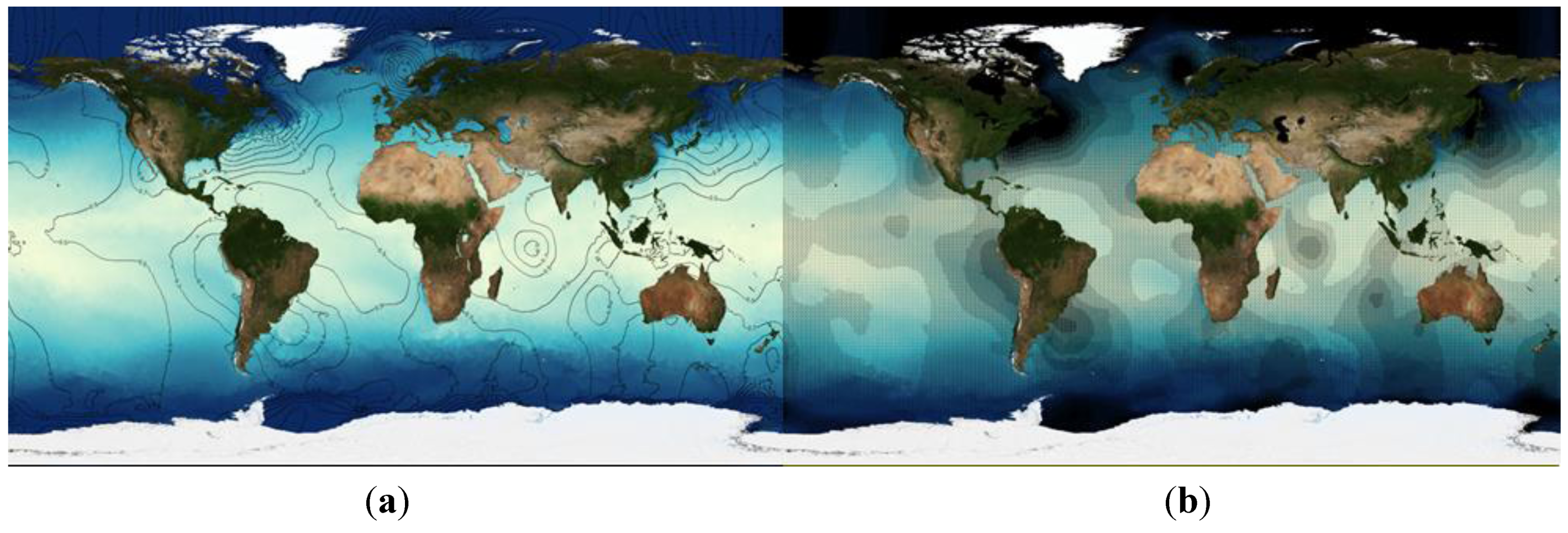
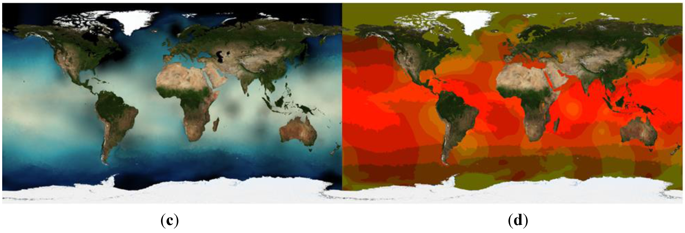
Figure 1.
Sample visualisations of sea surface temperature and its uncertainty from the Sea Surface Temperature dataset from the European Space Agency’s Climate Change Initiative (CCI-SST) dataset [
19], generated by the ncWMS-Q software (see
Section 6.1) using the proposed extensions to the Symbology Encoding (SE) specification (see
Section 5.8). From top left: (
a) temperature encoded as lightness of colour, with overlain contours of its uncertainty (variance); (
b) uncertainty represented through successive levels of stippling, with denser stippling representing high uncertainty; (
c) uncertainty represented as black shading; (
d) use of a bivariate colour map, with temperature encoded as brightness and uncertainty encoded as colour saturation.
Note that early drafts of WMS-Q attempted to achieve the same goal using a displayable Layer at the variable level, which was allowed to contain children representing its components. However, the WMS standard states that all Styles are inherited by child Layers. It would be inappropriate for Styles that are suitable for whole variables (probably defining compositions of components) to be inherited by Layers representing individual components (for example, a style that plots contours of uncertainty on top of a colour-mapped field would not be suitable for portraying a single component). Because of this, the Layer representing the variable cannot be displayable, therefore we make the Layer representing the whole Variable a displayable child, allowing it to contain a different set of Styles from its individual components.
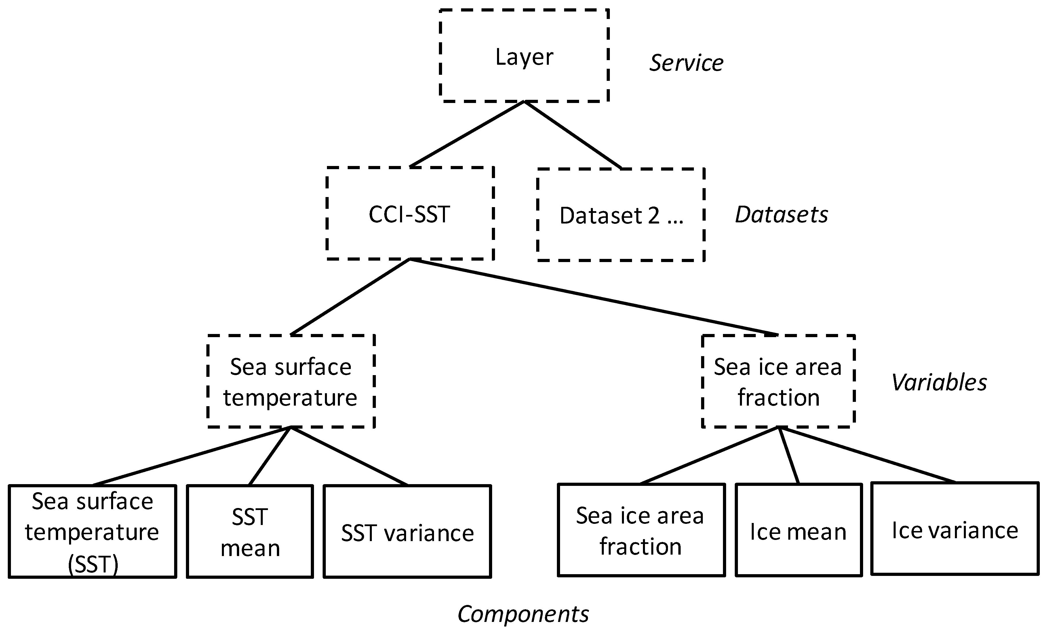
Example 1: In the CCI-SST dataset described in
Section 3 above, there is a “sea surface temperature” variable. The uncertainty of each sample is expressed using two components representing respectively the mean and variance of the variable. This is expressed in WMS-Q using a non-displayable Layer representing the variable, which is tagged with the “qualityCollection” and “statisticsCollection” Keywords. This Layer has three children: the first child represents the variable as a whole, and provides styles that enable the client to visualize the mean and variance together in a single image (e.g., using contours of variance overlain on a colour-mapped image). The remaining two children represent the mean and variance components respectively, and are tagged with Keywords containing the terms “mean” and “variance” from the UncertML vocabulary. This is represented in graphical form in
Figure 2. The complete WMS-Q service metadata document can be retrieved using this link:
http://ncwms.geoviqua.org/wms?SERVICE=WMS&REQUEST=GetCapabilities&VERSION=1.3.0&DATASET=cci-sst. A demo client showing the data can be found here:
http://ncwms.geoviqua.org/godiva2.html.
Figure 2.
Schematic representation of the structure of Layers in a particular “quality-enabled” profile of Web Map Service (WMS-Q) service instance, illustrating the Service-Dataset-Variable-Component hierarchy. Each box is a Layer in the tree: blue boxes represent non-displayable Layers, whereas orange boxes represent displayable Layers. The derivation of this hierarchy is given in
Section 5.5.
Example 2: We consider the “Landcover Classification” variable derived from Landsat in the Spanish National research project DinaCliVe. The classification method applied here combines common remote sensing classification techniques with the cadastre parcels and forces that each complete parcel is considered as a unity allowing statistical treatment of the pixels inside [
20]. The variable and its uncertainty are expressed at the sample level using several components. Some of them are categorical components such as the class with the most presence in the parcel and the second and third class present in that parcel. Some other components are continuous such as fidelity, representativity, promiscuity, entropy,
etc. (see
http://qualityml.geoviqua.org for their definition). The variable layer has several children: the first child represents the component that most users will want to see: the class with the most presence in the parcel. This is tagged with the Keyword
http://qualityml.geoviqua.org/1.0/values. The remaining classes help the user to understand the variability of the classification in the parcel and the confidence of the classification. All of them are tagged with the Keywords containing the right terms coming from the QualityML vocabulary. The complete WMS-Q service metadata document can be retrieved using this link:
http://www.ogc.uab.cat/cgi-bin/GeoViQUA/WMSQ/MiraMon.cgi?SERVICE=WMS&VERSION=1.3.0&REQUEST=GetCapabilities. A demo client showing the data can be found here:
http://wms-q-demo.geoviqua.org/geoviqua/wmsq/.
5.7. Behaviour of GetFeatureInfo
As mentioned in
Section 5.1 above, the WMS standard does not specify the data returned by the server in response to a GetFeatureInfo request. In WMS-Q, if GetFeatureInfo is requested for a layer that represents a Variable as a whole, we recommend that the server responds with a graphical or structured textual representation of the probability distribution function of the value of the variable at the requested point, if possible. If this is not possible, the server should respond with a document containing the values of each of the sample components at that point. This aspect of WMS-Q has not so far completely defined and will be refined in future versions.
5.8. Extensions to the Symbology Encoding Standard
There are a number of ways of portraying uncertainties in raster data, either as continuous or categorical fields. A full description of all options is beyond the scope of this paper, but common strategies include:
Portraying the “best estimate” as a colour-mapped image, overlain with contours showing a measure of data uncertainty (top left of
Figure 1).
As above, but uncertainty is represented through varying levels of stippling or texture (top right of
Figure 1), as used in the Assessment Reports of the Intergovernmental Panel on Climate Change (e.g., [
34]).
As above, with uncertainty represented using black shading, the opacity of which increases with data uncertainty (bottom left of
Figure 1).
Using a bivariate colour map (e.g., [
35]) in which the colour of a pixel is a function of two variables, the “best estimate” and the uncertainty (bottom right of
Figure 1).
Using glyphs (
i.e., small icons), the shape, size or colour of which can be mapped to different components of an uncertain variable. A special case of this is the use of “confidence triangles” (e.g., [
36]), which visualize the estimated spread of data by dividing the image into squares, each of which is divided into two triangles. The lower triangle is assigned a colour representing the lower bound of the variable, and the upper triangle is coloured according to the upper bound of the variable. The contrast in colours between the two triangles gives a visual estimate of the uncertainty.
The current version of the SE standard allows for only a limited number of means of visualizing raster data using the RasterSymbolizer. Data values can be mapped to pixel colours and the opacity of the image as a whole can be altered. Other functions in SE are oriented around optical remote sensing imagery (with assumed red, green and blue channels) or digital elevation models. Contours, stippling, bivariate colour maps or glyphs are not supported in SE. We therefore propose extensions to SE to support these portrayal types. For reasons of space, a full description of the implementation of these new styles is beyond the scope of this paper, but are described in a draft document at
http://www.geoviqua.org/Docs/03_ncWMS_Styling_Specification_1.0.pdf and are implemented in the ncWMS-Q software (see
Section 6.1 below and a test client at
http://ncwms.geoviqua.org/sldtest.html).
Clients can request that map images be generated using these new styles by crafting a SLD document using these new styles and passing it to the server. Alternatively, a server may offer named styles that implement these new styles, for convenience and simplicity (at the expense of some flexibility).
5.9. Mixing “Quality-Enabled” Data with “Non-Quality-Enabled” Data
In WMS-Q, not all Layers will necessarily have quality information (at the variable or sample level or either) attached. It is permissible to mix “quality-enabled” and “regular” layers in the same WMS service instance. The presence of MetadataURL links to metadata documents with quality indicators and the special keywords “qualityCollection”, “qualityComposition” or other keywords in the UncertML or QualityML vocabulary allow the client to detect the quality-enabled layers in a WMS service.
7. Integration of WMS-Q in a Quality Enabled Spatial Data Infrastructure
WMS-Q was developed in the context of the GeoViQua project (
http://www.geoviqua.org), which also developed several other components of a “quality-enabled” SDI. Although these components were originally designed and developed as enhancements to the Global Earth Observation System of Systems (GEOSS), they are more widely applicable.
Data cataloguing and discovery was implemented by enhancing the Discover and Access Broker (DAB) to produce a quality-enabled version (DAB-Q,
http://essi-lab.eu/do/view/GIcat). This harvests the WMS-Q service metadata (“Capabilities”) documents and maps the different Layers there present into ISO 19115 documents, which form the basis of the data catalogue. Those metadata ISO documents can be then used in the GEO Portal (
http://www.geoportal.org) to find datasets which are quality enabled. Thus, when a WMS-Q enabled dataset is found in a search, in addition to all the current links presented, links to the different variables and their quality components are given to the user.
A prototype to discover datasets with certain statistical properties was implemented, allowing searches that are aware of the dataset quality (for example, standard deviation less than 1 meter). The final port of this quality enhanced implementation to the GEO Portal search engine is to be done.
8. Discussion and Future Work
This paper introduces WMS-Q, a profile of the WMS standard that provides a mechanism for communicating data quality. The essential features of the profile are:
Communication of data quality at the level of datasets, variables and individual samples
Re-use of concepts from related standards and vocabularies, including UncertML and QualityML, using the WMS Keyword tag to communicate the quality and uncertainty of a measured variable.
Full compatibility with version 1.3.0 of the WMS standard.
Extensions to the SE specification to give greater control over visualizations of uncertain components.
This profile was developed in the first version as an OGC public engineering report [
39]. However, during further test in the GeoViQua project, some problems in the document were detected and solved. The results of these modifications were presented here and also in the WMS Standards Working Group that is now considering it as a possible OGC standard profile.
We have presented examples of use of the profile for two raster datasets: one representing continuous data (sea surface temperature) and one representing categorical data (land use classification). Further extensions to the SE specification could be devised in order to support more ways of visualizing uncertainty, such as the “uncertainty ribbons” and “graduated glyphs” described in [
7]. Some extensions to vector data was also tested in the GeoViQua project and will be investigated in future work, building on approaches such as those described in [
11].
Parallel work has extended these concepts to the Web Map Tile Service (WMTS) standard and will be described in future publications. WMTS was developed reusing many concepts of WMS but with scalability and performance in mind. Both have the concept of Layers and both deliver maps as a result. An important difference that is important for applying this profile is that layer nesting cannot be done in WMTS. Instead, the concept of themes was introduced, decoupling the layer definition from the layer interdependencies. A theme is defined as a tree structure that can contain other themes that can represent variables and layer references that can represent uncertainty components. This way, a quality theme can be defined to describe the sample quality components relation for a variable.
This paper focuses in discovery standards but many concepts could be reused in data access standards and services, such as the Web Coverage Service (WCS) standard. The version 2 [
40] of this standard has adopted a modular approach that allows for better extensibility. In WCS, GMLCOV [
41] (a GML application schema for coverages) is used to describe coverage offerings and it could be profiled to accurately identify uncertain variables and the components that convey them at the sample level. In addition, WCS operations could be extended to request the necessary quality and uncertainty components.
Recently, we have started to collaborate with weather forecasting agencies including MeteoFrance, the UK MetOffice, KNMI, DWD, ECMWF and AFWA, who are working together on a WMS best practice way to better communicate probability of forecasts resulting model ensembles, through WMS. These organizations are already providing WMS services and they have implemented their own solutions. By considering each ensemble result as a statistical sample and derived products as statistical probability distributions, we recognized the relevance of WMS-Q as a solution for ensemble standardization. We expect that the results of these discussions can converge in the use of an improved version of WMS-Q that fulfils the requirements of the weather and ocean forecasting community.


 ,
, 