Abstract
Expanding traditional time geography, this study examines personal exposure to air pollution and personal pollutant intake, and defines personal health danger zones by accounting for individual level space-time behavior. A 3D personal air pollution and health risk map is constructed to visualize individual space-time path, personal Air Quality Indexes (AQIs), and personal health danger zones. Personal air pollution exposure level and its variation through space and time is measured by a portable air pollutant sensor coupled with a portable GPS unit. Personal pollutant intake is estimated by accounting for air pollutant concentration in immediate surroundings, individual’s biophysical characteristics, and individual’s space-time activities. Personal air pollution danger zones are defined by comparing personal pollutant intake with air quality standard; these zones are particular space-time-activity segments along an individual’s space-time path. Being able to identify personal air pollution danger zones can help plan for proper actions aiming at controlling health impacts from air pollution. As a case study, this paper reports on an examination and visualization of an individual’s two-day ozone exposure, intake and danger zones in Houston, Texas.
1. Introduction
Air pollution refers to the contamination of the atmosphere that may lead to adverse health effects to human beings, animals, plants, and environments [1]. The U.S. Environmental Protection Agency (EPA) has set National Ambient Air Quality Standards (NAAQS) for six common air pollutants (i.e., criteria pollutants), including particulate matter (PM), ground-level ozone (O3), carbon monoxide (CO), sulfur oxide (SOx), nitrogen oxide (NOx), and lead. If the levels of one or more pollutants are higher than the EPA standards, the air quality is considered bad and may cause severe health effects. PM and ground-level O3 are the most widespread health threats to human beings. High air pollution exposure can cause an increase in morbidity and mortality rates; recent evidences revealed that accumulated exposure to low air pollution can also produce severe health effects, including death, disability, and illness [2].
This study focuses on examining the spatial-temporal dynamic patterns of personal air pollution exposure and intake by using an extended time geography approach and 3D geovisualization. This paper is developed to address three inter-mingled questions—What is the air pollution level in the ambient air? What is an individual’s exposure to polluted air when personal spatiotemporal trajectory and activities are considered? And what are an individual’s personal health danger zones due to air pollution?
1.1. AQI for Ambient Air Quality and Individual Health Impact
Air quality index (AQI) indicates the degree of air pollution and the potential health effects from air pollution. It is a tool designed to help the public understand the local air quality and the adverse health effects of ambient air [3]. AQI is reported as a positive number, and its standard varies across different nations. The U.S. EPA calculates AQI based the concentration of major air pollutants, i.e., ground-level O3, PM2.5, PM10, carbon monoxide (CO), nitrogen dioxide (NO2), and nitrogen oxide (NOx) [4]. AQI is reported following a six-color scheme from green to maroon, corresponding to good air quality to hazardous air quality, respectively (Table 1) [5].

Table 1.
The U.S. AQI standard (Source: EPA 2009).
| AQI | Health Concern | Color | Explanation |
|---|---|---|---|
| 0–50 | Good | Green | Clean air, no health risk |
| 51–100 | Moderate | Yellow | Light air pollution, little health risk |
| 101–150 | Unhealthy for sensitive groups (USG) | Orange | Only sensitive groups are affected |
| 151–200 | Unhealthy | Red | Unhealthy air for everyone |
| 201–300 | Very Unhealthy | Purple | Serious health effects for everyone |
| 301–500 | Hazardous | Maroon | Severe adverse health effects, even death |
Air pollutants concentrations are measured at many locations, local and nation-wide. Separate AQI is calculated for each pollutant using the standard EPA formula below:
where I is the AQI value for a pollutant of concern, C is the air pollutant concentration, Bh is the high break point (≥C) for the concentration of the pollutant, Bl is the low break point (≤C) for the concentration of the same pollutant, Ih is the high AQI limit corresponding to Bh, Il is the low AQI limit corresponding to Bl. Note that, given an air pollutant, EPA has defined the threshold concentration values of Bh, Bl, and the corresponding AQI values of Ih and Il to reflect the health impacts of the pollutant [5]. The highest AQI value during a day is recorded as the AQI of that day. The hourly reports for local and national AQI (such as PM2.5, O3, and PM2.5-O3 combined) are updated and published through multiple channels [6,7].
AQI maps show air quality across a mapping area by using the AQI six-color scheme (as Table 1). These maps are usually used for AQI reporting and forecasting. For example, a public web site—WWW.AIRNOW.GOV—provides near real-time hourly AQI maps for the U.S. and AQI readings for major U.S. cities. Figure 1 shows one such map.

Figure 1.
A U.S. national PM2.5-O3 combined AQI map (Source: AIRNow 2011).
Figure 1.
A U.S. national PM2.5-O3 combined AQI map (Source: AIRNow 2011).
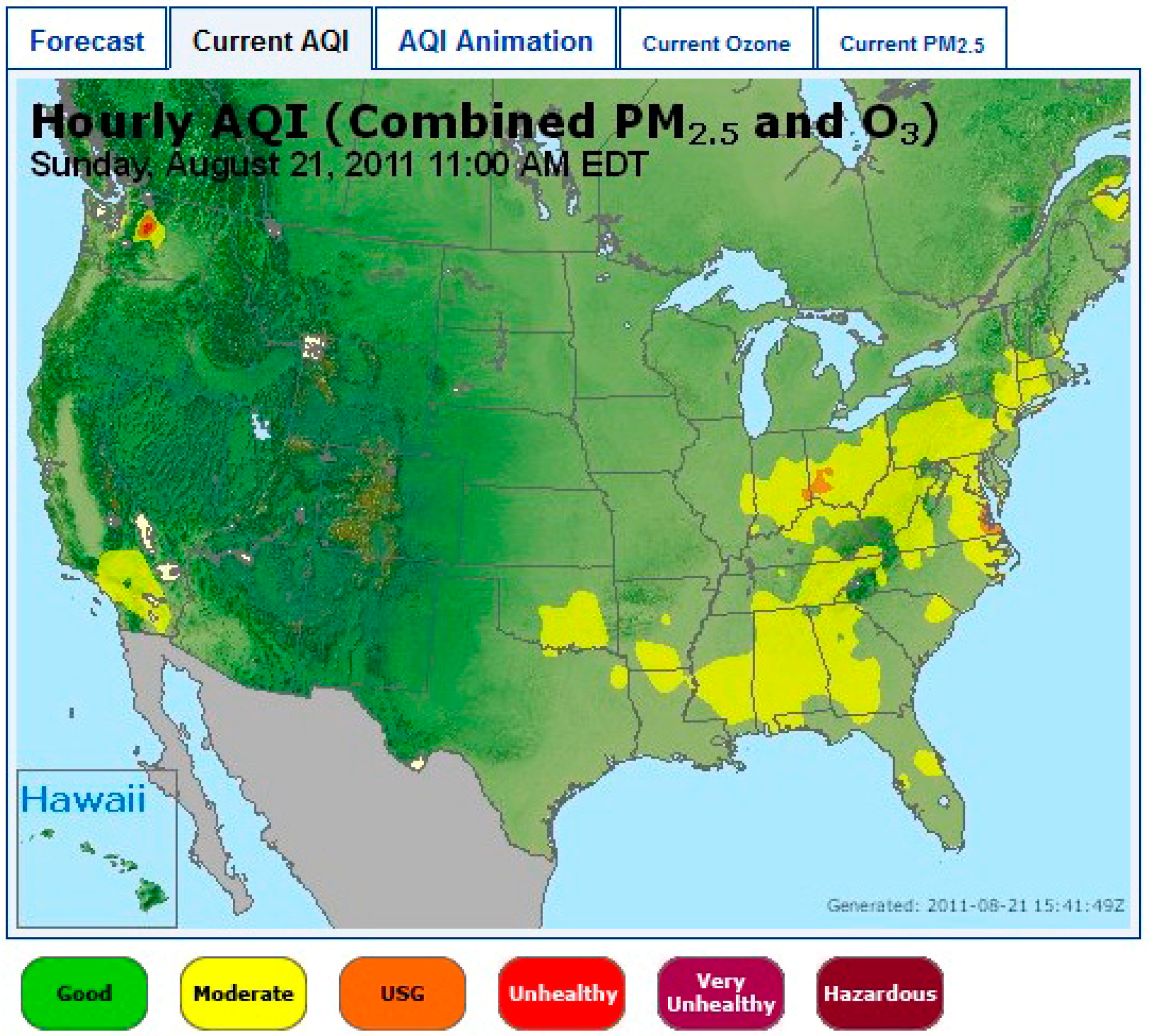
AQI maps provide a good visualization of air quality and its variation across the mapping area. However, it is very limited for assessing air quality and its adverse health effects for individual human beings. The limitation is related to both the spatial and the temporal resolution of the AQI values. First, most AQI maps show AQIs on a city, township, or county level. To derive directly from these maps the health implication for individuals is subject to ecological fallacy. As Kwan [8] pointed out, there is a clear rising need for the assessment of health effects to gear away from deriving environmental effects on the individual level from an aggregated neighborhood level and to move towards assessing the health effects on a personal level. There has emerged in the past few years a number of studies and research projects that piloted the exploration of assessing individual level health effects of air pollution, although most of them are limited in both space and time scales partially due to the technical challenges related to sensors and data collection [9]. Second, AQI maps are 2D maps that reflect the spatial variation of air quality and its health effects at one specific time point or as an average over a period of time. However, air quality and its health effects are present continuously through time. The traditional AQI values and maps lack the capability to assist continuous assessment of air quality and health effects.
The traditional AQI is further limited for personal level health effects assessment due to its negligence of the individual characteristics, including individual’s activities and biophysical characteristics. The health implication of air pollution is as much an individual level impact as it is for the general population. While an elevated concentration of a certain pollutant may impact human beings’ health condition in a similar way, the adverse health effect on an individual is more a function of the type and patterns of the activities an individual conducts and his/her physical and biological characteristics. Therefore, as dynamic as the spatiotemporal patterns of air pollution and thus AQI value, individuals can benefit greatly from an individualized health effects assessment that specifically reflects the patterns and sequences of individual level space-time trajectory and activities.
1.2. Personal Exposure to and Intake of Polluted Air
Human exposure to air pollution occurs when contacting with air contaminants in a place and at a time [10,11]. Personal exposure can be measured either directly (e.g., personal sampling and biological marker measurement) or indirectly (e.g., ambient measurement/modeling and survey) [12]. Among the different measurement methods, personal sampling has a high accuracy. It is often used to collect data on air pollutant concentration in an individual’s immediate surroundings, personal exposure frequency, and exposure duration. Personal exposure to air pollution is an accumulated process that is related to not only air pollutant concentration but also the periods of time and sequence of locations of exposure.
Personal air pollutant intake directly contributes to the health effects at individual level. It is related to a series of environment-human interaction processes, including human contacting with the air pollutants, the concentration of the pollutants over space and time, and the absorption of the pollutants by human body. Among the different absorption ways, inhalation is the major means for air pollutants to enter human body [13]. Inhalation rate varies across individuals; it changes for the same individual across different situations. Besides, health effects of air pollution are related to both air pollutant exposure and individual level biophysical characteristics [14]. Table 2 was adapted from Holmes [15]; it reports on the air inhalation rate when the different types of physical activities and the different population groups are considered. Equation 2 explains how air pollutant intake can be estimated by considering pollutant concentration, individual inhalation rate, and individual exposure time and place:
where AIp indicates personal air pollutant intake (inhalation dose), C(t,l) is air pollutant concentration at time t and location l, R(t,l) is the real-time inhalation rate, dt is the time span (t1 to t2) of exposure, and dl is the location unit that collectively make the whole spatial trajectory (l1, l2).
Table 2.
Individual average air intake volume per minute (adapted from Holmes 1994 [15]).
| Group | Staying/Sleeping/In Car | Walking | Running/Cycling | Playing/Light Physical Labor | ||||
|---|---|---|---|---|---|---|---|---|
| Speed | Air Volume | Speed | Air Volume | Speed | Air Volume | Speed | Air Volume | |
| Children | 24 | 5–10 | 1–5 | 12.5–17.5 | 5–24 | 30–35 | <2 | 15–20 |
| Adult females | 24 | 5–10 | 1–5 | 17.5–22.5 | 5–24 | 45-50 | <2 | 15–20 |
| Adult males | 24 | 7.5–12.5 | 1–7 | 25–35 | 7–24 | 55–60 | <2 | 20–30 |
Unit: Speed (km/h), Air volume (liter)
2. Time Geography and Individual Space-Time Behavior Analysis
Individual space-time behavior refers to an individual’s movements and activities through time and across space. There are several aspects for describing individual space-time behavior, such as travel type, space-time trajectory, stops, duration, speed, and sequence [16]. Two groups of quantitative methods are commonly employed for individual space-time behavior analysis. One group takes a holistic view to analyze the trajectories or activity types, such as the approach by location sequence alignment [17]. The other group focuses on a certain aspect of individual behavior, such as the travel distance from major employment centers [18]. As pointed out in literature [16], many quantitative analyses of individual space-time behavior are limited because they rely on a series of isolated events to describe continuous space-time behavior. In other words, discrete spatial variables (e.g., dividing space into several homogeneous zones) and temporal variables (e.g., using hourly average activity instead of real-time activity) are used, and these discrete variables may lead to errors and are subject to issues such as the Modifiable Areal Unit Problem (MAUP) [8]. Therefore, most studies failed to reflect the full picture of individual space-time behavior (and the environment effects of these behavior) due to the limitation of the spatial and temporal analysis scheme.
Swedish geographer Torsten Hägerstrand developed the conceptual framework of time geography in the late 1960s. According to Hägerstrand [19], individual space-time behavior is always limited by a series of constraints of space and time, including authority constraints, capability constraints, and coupling constraints. Under these constraints, an individual travels through a 3D space-time cube, i.e., a two-dimensional space and a one-dimensional time. The 3D travel trajectory in this cube is called a space-time path (Figure 2). Space-time prism [19] was developed to define an individual’s travel possibility across space and through time. The concept of space-time prism was introduced into Geographic Information System (GIS) by Miller [20] more than two decades later to examine the spatiotemporal accessibility of individuals.
According to time geography, spatiotemporal events are presented through three components—theme, location, and time; these components are measured, controlled, and fixed respectively, to form different combinations [21]. For example, in a regional air pollution map, location is fixed, time is controlled, and theme (i.e., pollution) is measured. However, due to the limitation in information and visualization technologies as well as that in computation power, Hägerstrand’s time geography has been mostly a framework for a long time. Individual space-time behavior has been studied at relatively coarse spatial scales and discrete time slices until recently. The visualization has been mostly 2D-maps showing distribution across space at selected time points.
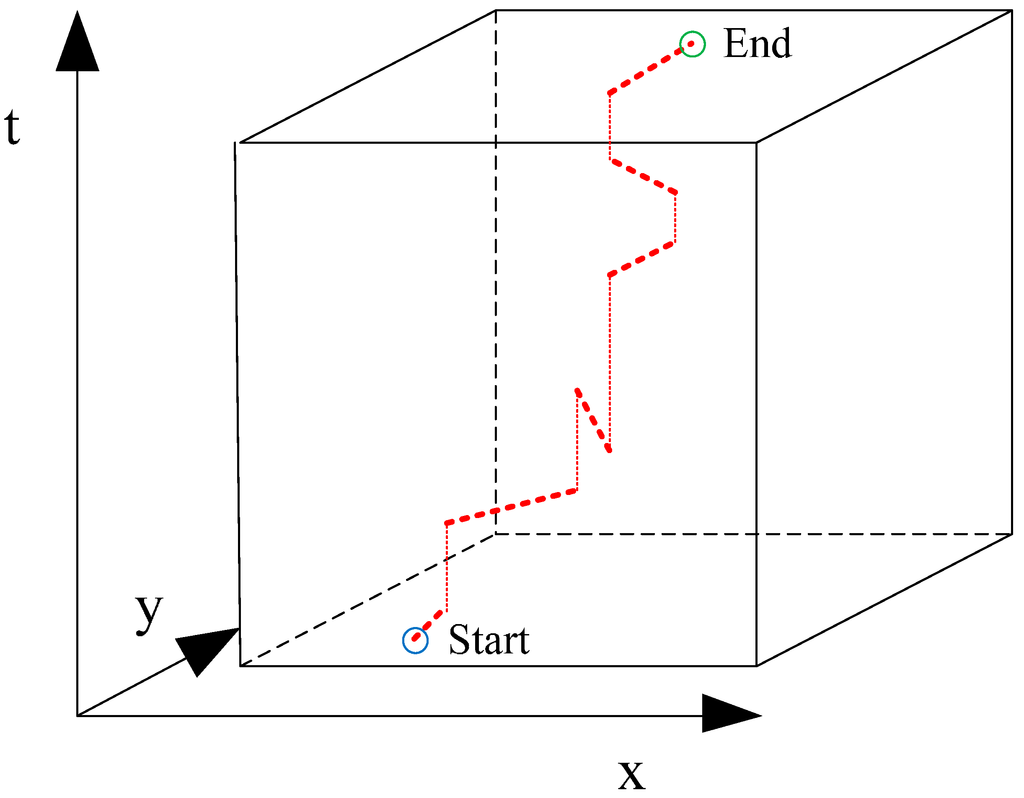
Figure 2.
A space-time path in a time geography space-time cube.
Figure 2.
A space-time path in a time geography space-time cube.

With the development in GIS and visualization technologies in the 21st century, important progresses were made to profile individual space-time behavior using GIS-based 3D modeling and visualization. For example, Kwan [22] explored the activity-travel behavior of more than 10,000 individuals in Portland, Oregon. The space-time behaviors of these individuals were mapped using a GIS-based 3D geovisualization where individual space-time paths was integrated with the base map. Shaw and Yu [23] believe that individual’s daily activity and travel behavior are highly influenced by modern Information and Communication Technologies (ICT), and therefore the virtual space makes a significant component for an individual’s living space. They developed individual space-time path maps that integrate individual’s virtual activities (such as teleconference and mobile phone calls) with his/her physical activities (such as working, commuting trips, and meeting). Chen et al. [24] developed an ArcGIS space-time extension—Activity Pattern Analyst (APA) to visualize and analyze individual space-time behavior aiming at exploring the hidden aggregate patterns in large spatiotemporal datasets.
In the last ten years or so, development in hand-held Global Position System (GPS) and that in ICT (especially mobile and wireless communication technologies) have greatly enhanced the advancement in pervasive location acquisition [25]. This made the data collection for individual level space-time trajectory more practical and benefited the space-time analysis of individual behavior. Hägerstrand’s space-time cube was implemented by recent studies for both visualization (e.g., [26]) and analysis (e.g., [27,28]) of individual’s space-time trajectories. Rossmo et al. [29] analyzed the travel patterns of 19 parolees and mapped their 3D space-time paths using GeoTime software; their individual space-time trajectory data were collected by portable GPS units. However, these studies examined individual-level space-time behavior by focusing mostly on an individual’s space-time trajectory while considering away the dynamics of individual-environment interaction and environmental exposure. A trajectory is described as a collection of tri-tuples, I (xi, yi, ti). The environment impacts along the trajectory are either overlooked or treated as constant. This approach is limited for modeling the dynamic nature of the interaction between an individual and the environment, which is critical for understanding individual-level environment exposure and the related health effects. The dynamics of an individual’s exposure to air pollution as one moves along a spatiotemporal trajectory must be properly accounted for in order to accurately assess the health effects of air pollution on an individual.
There is a lack in literature to connect an individual’s spatiotemporal trajectory (i.e., space-time path in Hägerstrand’s space-time cube) with the changing nature of his/her environment exposure in general and air pollution exposure in particular. To the authors’ knowledge, the only study that has explicitly developed the traditional time geography space-time cube to include a description of the environment dynamics was Fang and Lu [30]. Hägerstrand’s space-time cube was extended to an air pollution cube of space-time in this study where the base 2D map shows the air pollution concentration and variation across space and the third-dimension shows the progress of time along which the spatial distribution of air pollution concentration changes. Following Fang and Lu [30], we propose that an individual’s interaction with environment along a particular space-time path through a space-time cube can be modeled as a collection of qua-tuples, I (xi, yi, ti, Ei), where Ei represents the environmental exposure of an individual at i, a particular space-time position. For air pollution and personal health effect study, Ei is defined collectively by the air pollutant concentration, personal pollutant intake, and personal physical activity and biophysical characteristics. The dynamics of Ei determines the continuous change of the health effects of air pollution for a person given his/her space-time behavior in the study area and during the study period.
The study reported below seeks to expand the traditional space-time path in time geography to account for the dynamics of environment exposure of an individual through space and time. Using data from portable GPS and air pollution sensors, this study presents an approach to measure individual-level air pollution exposure by considering an individual’s space-time behavior. The study further seeks to assess individual-level health effects by defining individual-level air pollution danger zones to reflect the violation of EPA’s air quality standards.
3. An Experiment in Houston
On 27 and 28 December 2010, an adult male volunteer traveled in Houston, Texas and collected two essential data sets and some supplementary data. The first data set was real-time air pollution level data, particularly ozone (O3) concentration level. A BW GasAlert Extreme single gas detector (O3) with 10 ppb increments was used as the air pollutant sampler. This sampler was carried by the data collector to record pollutant concentration data at his immediate surroundings. The second data set was individual space-time trajectory data. A Garmin eTrex Vista H handheld GPS navigator was used to record travel data (i.e., travel trajectories, travel speeds, and stops). Both instruments were set to collect data at a 10-s interval. The volunteer also maintained a travel diary describing the location and nature of activities during the data collection period.
The volunteer’s space-time travel data was processed using ArcScene in ArcGIS software package. Figure 3 is an ArcScene generated 3D map showing the individual’s space-time path as laid on top of a Houston base map. The vertical dimension (z) represents the two-day travel time; the horizontal dimensions (x, y) represent the space of Houston, Texas. The real-time O3 concentration data for the individual’s immediate surroundings was downloaded from the portable sensors. The real-time AQI values along the individual’s space-time path were calculated following Equation (1). The real-time personal O3 intake rates were computed using Equation (2) by considering the real-time ambient O3 concentration data, individual physical activities (as recorded in travel diary), and physical activity-related air intake rate (as listed in Table 1). When the real-time personal O3 intake volume during a unit time was higher than EPA air quality standards, the person was determined to be in an air pollution danger zone.

Figure 3.
The space-time path of the volunteer in Houston, Texas on 27 and 28 December 2010.
Figure 3.
The space-time path of the volunteer in Houston, Texas on 27 and 28 December 2010.
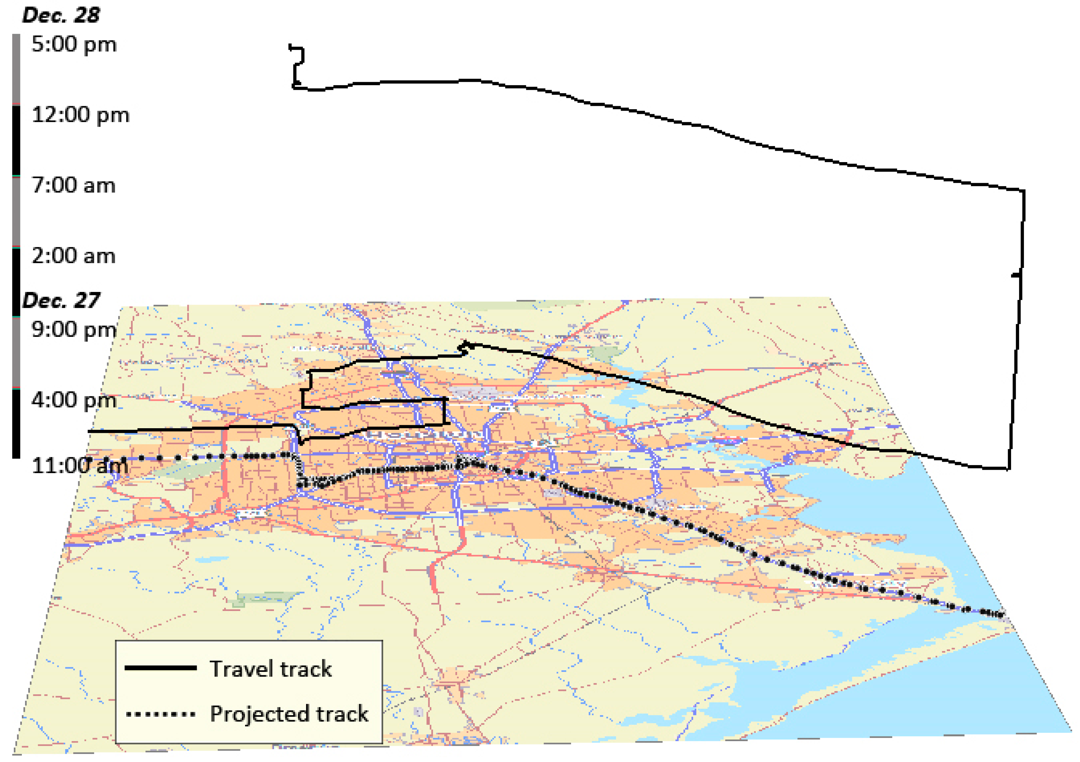
The recorded O3 concentration values ranged from 20 ppb to 80 ppb on 27 and 28 December 2010. During the afternoon of 27 December, the measured O3 concentration values varied a lot. By connecting to the GPS data and the travel diary, it was found that O3 concentration was mostly at medium level when the volunteer traveled on major roads (e.g., Interstate Highway 10, Interstate Highway 45, and W Sam Houston Parkway S); O3 concentration was low when the volunteer traveled on minor roads or stayed indoors (e.g., shopping and rest). This indicates that O3 concentration level is closely related to traffic emissions in urban Houston. During the night of 27 December and the morning of 28 December, the O3 concentration level remained low and stable. The volunteer stayed inside mostly during this time period except for a 40-min outdoor morning exercise, which included jogging and walking. When the volunteer traveled through the city of Houston along highways during midday on 28 December, the O3 concentration was recorded as being relatively high. It was low in the afternoon of 28 December, during which time the volunteer traveled short distances while conducting a variety of activities, including staying, walking, and running.
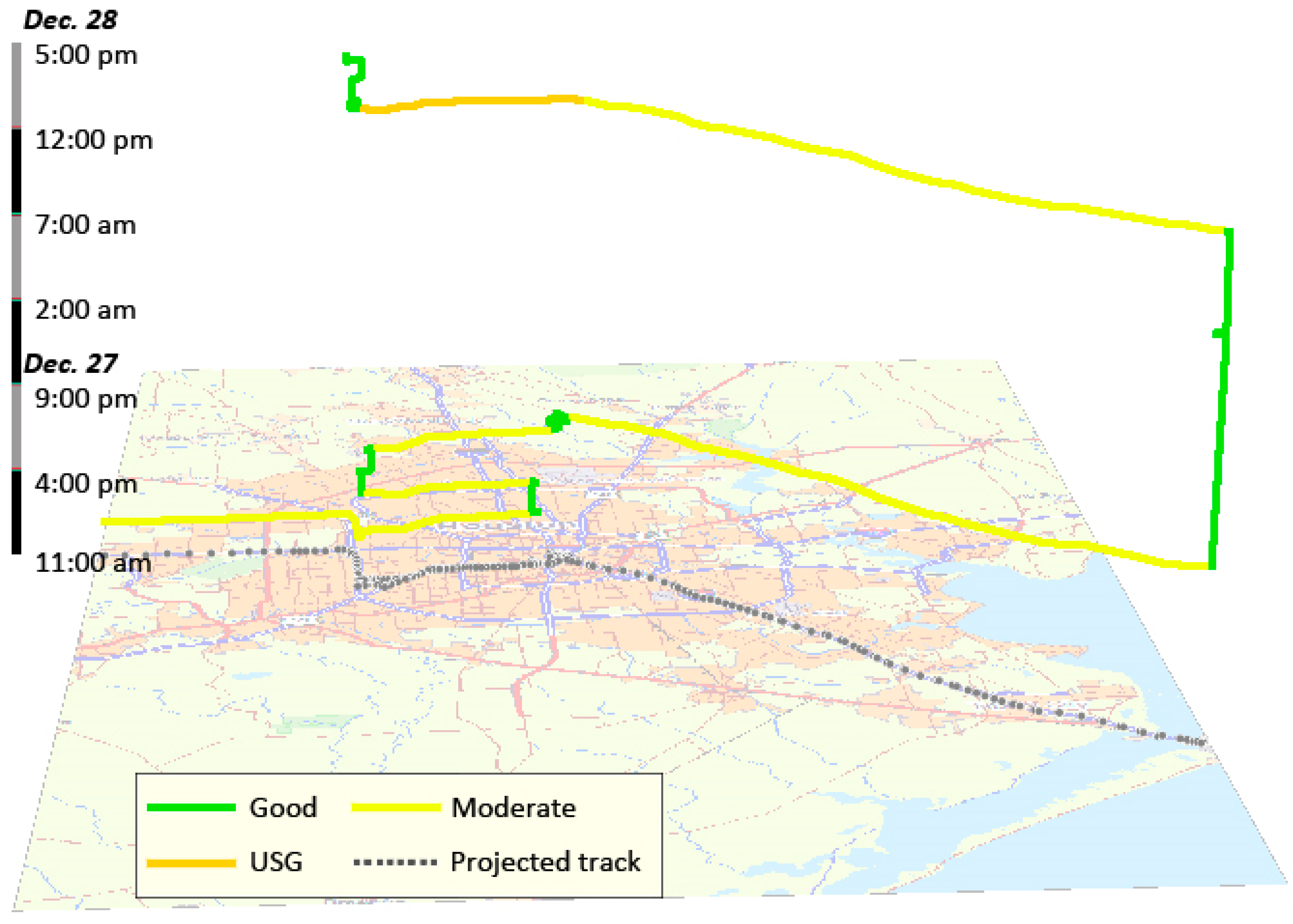
Using the recorded O3 concentration data, real-time AQI values were calculated for the volunteer throughout the study period. Following the U.S. AQI standard (see Table 1), different colors are used to visualize the volunteer’s real-time personal AQIs. In Figure 4, green indicates good air quality (AQI range: 0–50), yellow indicates moderate air quality (AQI range: 51–100), and orange indicates that the air quality is unhealthy for sensitive groups (USG) (AQI range: 101–150). The continuous AQI values and its color scheme is an important individual property that is uniquely associated with the volunteer’s space-time trajectory. As discussed in the previous section, this aspect can be represented as the Ei for the individual’s space-time path that is made up of instances I (xi, yi,, ti, Ei). Figure 4 is a visualization of the dynamic individual-environment interaction along the space-time path of the volunteer; particularly, his real-time AQI along the space-time path is visualized together with his position in the space-time cube.

Figure 4.
The volunteer’s space-time path with personal AQIs in Houston, Texas on 27 and 28 December 2010.
Figure 4.
The volunteer’s space-time path with personal AQIs in Houston, Texas on 27 and 28 December 2010.
The volunteer’s real-time personal O3 exposure (i.e., O3 concentration in immediate surroundings), real-time AQIs, and real-time O3 intake rates are plotted together in Figure 5. Note that the three measures were plotted to be compatible along the y-axis for visualization purpose. As AQIs are directly related to O3 concentration, the variation of the volunteer’s real-time personal AQIs is similar to that of the concentration of O3. However, there may be a big difference between the pollution concentration level (i.e., concentration of O3) and the pollutant intake level (i.e., O3 intake rate), as shown in Figure 5 for the mid-afternoon on 27 December. The nature of individual activities during this time is the major cause for this difference. Given a pollutant concentration level, the different types of activities required different levels of air intake, leading to different pollutant intake levels. This clearly shows the importance of understanding the dynamics of individual-environment interaction along a space-time path, which is the Ei in the qua-tuples of I (xi, yi, ti, Ei).
Figure 5 shows that the volunteer’s O3 intake rates were higher and more unstable during the daytime. The volunteer visited different places and conducted different types of daytime activities, including walking, running, and staying. These activities changed his breathing rate and resulted in increased and changing levels of O3 intake. During the nighttime, the volunteer stayed indoor with low-level physical activities, leading to low and stable O3 intake rates.

Figure 5.
The volunteer’s real-time air pollution exposure, intake, and AQI values during the 27–28 December 2010 data period in Houston, Texas. (a) O3 intake rate (10−8 L/min); (b) AQI; (c) measured O3 concentration (ppb).
Figure 5.
The volunteer’s real-time air pollution exposure, intake, and AQI values during the 27–28 December 2010 data period in Houston, Texas. (a) O3 intake rate (10−8 L/min); (b) AQI; (c) measured O3 concentration (ppb).
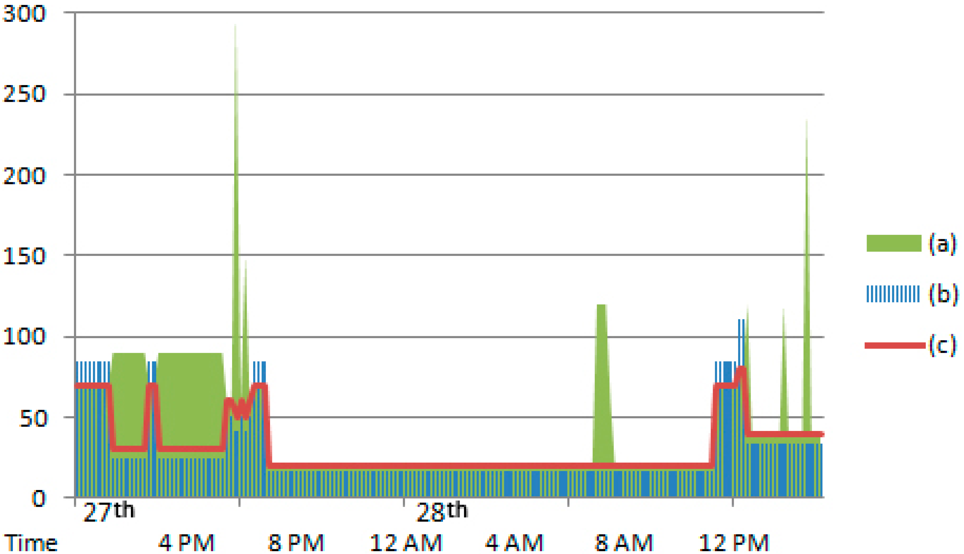
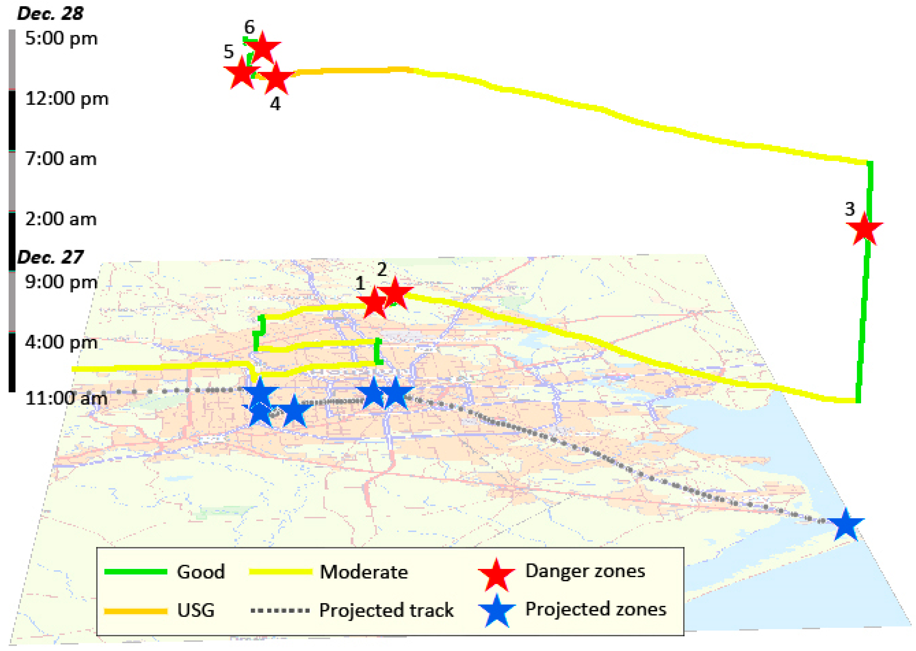
A total of six peaks of O3 intake rate (i.e., intake rates > 10−6 L/min) can be identified from Figure 5. Two peaks were occurred in the afternoon of 27 December, one peak in the morning of 28 December, one peak in the noon of December 28, and two peaks in the afternoon of December 28. By cross-referencing GPS trajectory data, the six peaks can be registered to specific positions in the space-time cube. Figure 6 highlights these corresponding six nodes as the high O3 intake danger zones along the volunteer’s space-time path. These zones signify the dangerous health risk segments in the individual’s space-time behavior during the study period. Note that some of these danger zones fall onto the space-time segments where AQIs were not good, but others fall onto AQI safe segments along the volunteer’s space-time path. The air quality at zone 1 and 2 was moderate (AQI color: yellow); the air quality at zone 3, 5, and 6 was good (AQI color: green); the air quality at zone 4 was unhealthy for sensitive groups (USG) (AQI color: orange). This manifests that even if the air quality is good, strenuous exercise may lead to inhalation of excessive air pollutants, and therefore exposure an individual to dangerous level of pollutant intake. On the other hand, when air pollutant concentration is relatively high and AQI is not good, maintaining inactive or less active physical activities so a minimum amount of pollutant entering into one’s body may be an effective measure for alleviating the adverse health effects of air pollution.
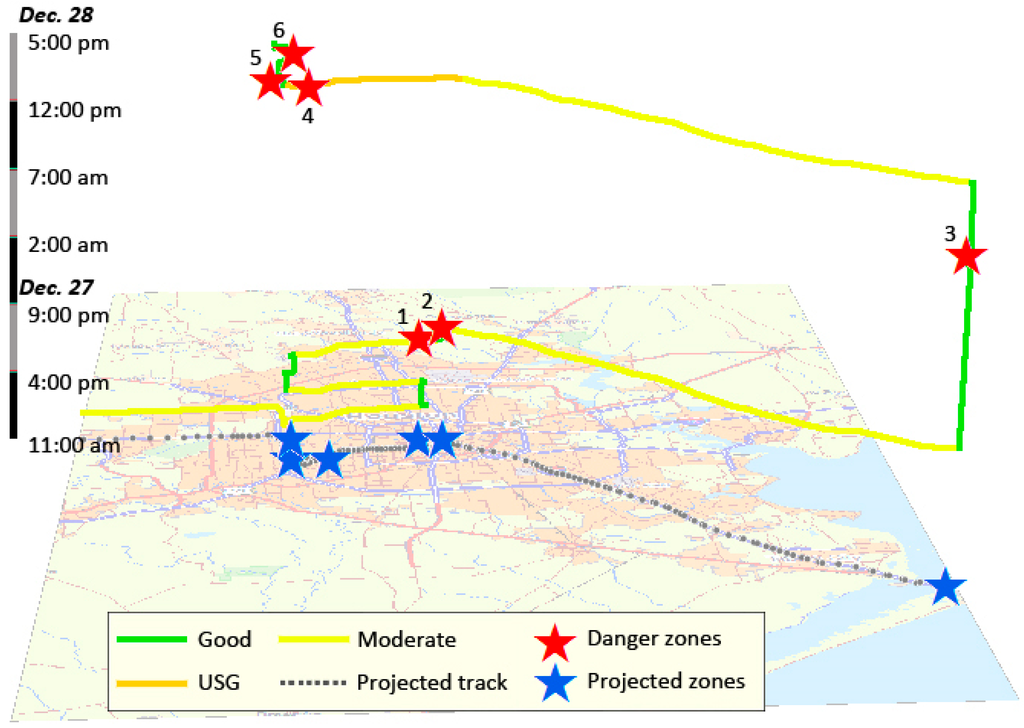
Figure 6.
The personal air pollution danger zones for the volunteer in Houston, Texas on 27 and 28 December 2010.
Figure 6.
The personal air pollution danger zones for the volunteer in Houston, Texas on 27 and 28 December 2010.
4. Conclusions and Discussion
To assess personal health effects of air pollution, two steps are essential: to quantify personal ambient air pollution concentration, exposure duration and pollutant intake, and to evaluate the related personal health effects by considering personal space-time behavior. This paper showcases how an individual-level assessment of air pollution exposure and health effects can be evaluated through systematically integrating personal level data collection, space-time modeling, and geovisualization technologies. First, space-time trajectory information must be added to air pollution data in order to depict where, when, and how much an individual is exposed to air pollution. Real-time air pollution concentration data can be collected with ease using a portable air pollutant sensor. But they cannot be linked directly to personal space-time behavior. To solve this problem, the individual space-time trajectory data was collected by a portable GPS unit and was linked to air pollution data. Second, a 3D modeling and visualization approach was developed based on time geography framework to model a space-time cube, a space-time path within the cube, and the dynamics of individual-environment interaction along the path. The environment variation within a space-time cube and the dynamics of individual-environment interaction along a space-time path are not accounted for by the traditional time geography. This study models the space-time path as a collection of qua-tuples, I (xi, yi, ti, Ei), where Ei represents environmental exposure at space-time point i. In the case of air pollution and individual health effect, the environmental exposure can be defined by the air pollutant concentration level and the pollutant intake rate (which is related to personal behavior and individual physical situation) along the space-time path. The approach of qua-tuples in space-time cube illustrates an effective measure to address the uncertain geography context problem (UGCoP) as identified by Kwan [31]. Third, based on the above two advancements, the proposed approach in this paper assesses personal level health effects of air pollution by considering air pollutant intake of an individual, which is determined by air pollution concentration, personal space-time trajectory, and personal activities throughout the trajectory. Air pollutant concentration levels in an individual’s immediate surroundings were converted to space-time path AQI values (Figure 4); air pollutant intake was estimated using information from personal travel diary (Figure 5); personal air pollution health danger zones (Figure 6) were identified by considering air pollution and personal space-time behavior.
An individual’s air pollution exposure changes through space and time, and it changes differently from his/her pollutant intake. In the case study, the O3 concentration level for the volunteer’s ambient air showed some regularity. When the volunteer drove along major roads, the O3 concentration was medium to high level; when he stayed inside and walked/jogged in shopping/residential areas, the concentration remained low. This pattern may suggest the important role of traffic emission to elevated O3 levels. Compared to O3 concentration, the volunteer’s O3 intake rates varies largely (i.e., ranging from 2 × 10⁻⁷ L/min to 30 × 10−7 L/min). Figure 5 and Figure 6 revealed that the volunteer’s O3 intake had six peaks, indicating air pollution health danger zones. Five of the danger zones (zone 1, 2, 4, 5, and 6) are in the downtown area of Houston and one (zone 3) in Galveston, Texas. The downtown danger zones mostly highlight the volunteer’s walking activities, and the Galveston danger zone represents the volunteer’s running activity. The health danger zones represent the space-time-behavior segments along an individual’s space-time trajectory where his/her personal health impact from air pollution was high. It is very important to understand that these danger zones may not fully agree with the personal AQI color zones. This is because AQI reflects concentration of pollutant in the ambient air, but the health danger zones are tailored to reflect the health effect from pollutant intake. Even though the pollutant concentration may not be as high, certain space-time activities may create personal danger zones due to the need for significantly elevated air intake.
The contributions of this study are mostly three-folds. First, time geography was extended to account for the dynamics of individual-environment interaction and was used as the framework for investigating the continuous change of personal exposure to and intake of air pollutant over space and time. Second, 3D maps were used to visualize personal exposure conditions. The 3D geovisualization modeled not only an individual’s space-time path but also the changing dynamics of real-time personal AQI. Third, personal air pollution danger zones are defined and visualized along the personal space-time path to connect personal space-time behavior with personal health effects. Applying this approach to a future prediction of air pollution scenario, one can model personal air pollution danger zones for an individual’s real or planned spatiotemporal activity trajectories. This can be used to assist an individual in selecting a spatiotemporal activity trajectory with the minimum adverse health effects. Therefore, the approach reported in this paper has a great potential in helping alleviate the adverse health effects of air pollution through managing individual-level space-time activities.
However, some limitations from the study should be noticed. First, the data accuracy for the empirical study in the paper is limited due to sensor precision. The increment of the portable O3 sampler was limited to 10 ppb, and any variation below this level was not detectable by the sensor. Second, the volunteer’s pollutant intake was estimated based on the past empirical findings about general population’s air inhalation rate. Future research should consider using portable breath sensor that can automatically and accurately record an individual’s breathe rate. Last, the limitation of the data collection means used in the reported pilot study must be recognized. It is impractical to expect the general public to carry both a GPS and a pollutant sensor while conducting daily activities. As pointed out by Fang and Lu [9], the research on real-time assessment of personal air pollution exposure and health effects are limited by the availability of sensors that can genuinely integrate location-detection and air pollutant sampling technologies. This technological limitation has been one major restriction for most of on-going or not-fully-implemented projects seeking to link air sensor to GPS (such as those reviewed in [19]). The focus of this paper is on the integration, analysis, and visualization of the related data for the purpose of analyzing personal health effects and health danger zones from air pollution. It is by no means the purpose of this study to showcase a GIS and air sensor integrated data collection approach.
This study pilots the investigation of personal air pollution exposure and intake, aiming at evaluating personal health effects of air pollution. Although only O3 was investigated by the empirical study, the approach can be extended to other pollutants when proper sensors are available and health standard related AQIs are defined. Our next step of work will include continuous search for and design of an improved data collection means to support extending the individual-level health effects analysis and health danger zone modeling to the general public in order to serve people with varied backgrounds and different space-time behavior patterns.
Author Contributions
Yongmei Lu led the design of the research. Tianfang Bernie Fang conducted the fieldwork and data processing. Both authors contributed to the writing of the paper. Yongmei Lu finalized the manuscript for submission.
Conflicts of Interest
The authors declare no conflict of interest.
References
- EPA. Air Pollutants. Available online: http://www.epa.gov/ebtpages/airairpollutants.html (accessed on 21 August 2011).
- Ostro, B.; Lipsett, M.; Reynolds, P.; Goldberg, D.; Hertz, A.; Garcia, C.; Henderson, K.D.; Bernstein, L. Long-term exposure to constituents of fine particulate air pollution and mortality: Results from the california teachers study. Environ. Health Perspect. 2010, 118, 363–369. [Google Scholar] [CrossRef] [PubMed]
- EPA. Air Quality Index—A Guide to Air Quality and Your Health; U.S. Environmental Protection Agency, Office of Air Quality Planning and Stadards, Outreach and Information Division: Research Triangle Park, NC, USA, 2014.
- EPA. What is Air Pollution? Available online http://www.epa.gov/airnow/airaware/day1.html (accessed on 21 August 2011).
- EPA. Technical Assistance Document for the Reporting of Daily Air Quality—The Air Quality Index (AQI); U.S. Environmental Protection Agency: Research Triangle Park, NC, USA, 2012.
- AIRNow. Local Air Quality Conditions and Forecasts. Available online: http://www.airnow.gov/index.cfm?action=airnow.main (accessed on 21 August 2011).
- EPA. Air Quality Index Report. Available online: http://iaspub.epa.gov/airsdata/adaqs.aqi?geotype=st&geocode=TX&geoinfo=st~TX~Texas&year=2008&sumtype=co&fld=gname&fld=gcode&fld=stabbr&fld=regn&rpp=25 (accessed on 21 August 2011).
- Kwan, M.P. From place-based to people-based exposure measures. Soc. Sci. Med. 2009, 69, 1311–1313. [Google Scholar] [CrossRef] [PubMed]
- Fang, T.B.; Lu, Y. Personal real-time air pollution exposure assessment methods promoted by information technological advances. Ann. GIS 2012, 18, 279–288. [Google Scholar] [CrossRef]
- Duan, N. Models for human exposure to air pollution. Environ. Int. 1982, 8, 305–309. [Google Scholar] [CrossRef]
- Lioy, P.J. Assessing total human exposure to contaminants. Environ. Sci. Technol. 1990, 24, 938–945. [Google Scholar] [CrossRef]
- Monn, C. Exposure assessment of air pollutants: A review on spatial heterogeneity and indoor/outdoor/personal exposure to suspended particulate matter, nitrogen dioxide and ozone. Atmos. Environ. 2001, 35, 1–32. [Google Scholar] [CrossRef]
- Weisel, C.P. Assessing exposure to air toxics relative to asthma. Environ. Health Perspect. 2002, 110 (Suppl. 4), 527–537. [Google Scholar] [CrossRef] [PubMed]
- Silverman, R.A.; Ito, K. Age-related association of fine particles and ozone with severe acute asthma in New York City. J. Allergy Clin. Immunol. 2010, 125, 367–373 e5. [Google Scholar] [CrossRef] [PubMed]
- Holmes, J.R. How much air do we breathe? In Measurement of Breathing Rate and Volume in Routinely Performed Activites; Adams, W.C., Ed.; National Technical Information Service: Springfield, VA, USA, 1994. [Google Scholar]
- Kwan, M.-P.; Ren, F. Analysis of human space-time behavior: Geovisualization and geocomputational approaches. In Understanding Dynamics of Geographic Domains; Hornsby, K., Yuan, M, Eds.; CRC Press: Boca Raton, FL, USA, 2008; pp. 93–113. [Google Scholar]
- Shoval, N.; Isaacson, M. Sequence alignment as a method for human activity analysis in space and time. Ann. Assoc. Am. Geogr. 2007, 97, 282–297. [Google Scholar] [CrossRef]
- Weber, J. Individual accessibility and distance from major employment centers: An examination using space-time measures. J. Geogr. Syst. 2003, 5, 51–70. [Google Scholar] [CrossRef]
- Hägerstrand, T. What about people in regional science. Pap. Reg. Sci. Assoc. 1970, 24, 1–12. [Google Scholar] [CrossRef]
- Miller, H. Modeling accessibility using space-time prism concepts within geographic information systems. Int. J. Geogr. Inf. Syst. 1991, 5, 287–301. [Google Scholar] [CrossRef]
- Langran, G.; Chrisman, N. A framework for temporal geographic information. Cartographica 1988, 25, 1–14. [Google Scholar] [CrossRef]
- Kwan, M.-P. Interactive geovisualization of activity-travel patterns using three-dimensional geographical information systems: A methodological exploration with a large data set. Transp. Res. Part C: Emerg. Technol. 2000, 8, 185–203. [Google Scholar] [CrossRef]
- Shaw, S.-L.; Yu, H. A GIS-based time-geographic approach of studying individual activities and interactions in a hybrid physical-virtual space. J. Transp. Geogr. 2009, 17, 141–149. [Google Scholar] [CrossRef]
- Chen, J.; Shaw, S.-L.; Yu, H.; Lu, F.; Chai, Y.; Jia, Q. Exploratory data analysis of activity diary data: A space-time GIS approach. J. Transp. Geogr. 2011, 19, 394–404. [Google Scholar] [CrossRef]
- Lu, Y.; Liu, Y. Pervasive location acquisition technologies: Opportunities and challenges for geospatial studies. Comput. Environ. Urban Syst. 2012, 36, 105–108. [Google Scholar] [CrossRef]
- Kraak, M.J. The space-time-cube revisited from a geovisualization perspective. In Proceedings of the Twenty-First International Cartographic Conference (ICC), Durban, South Africa, 10–16 August 2003; pp. 1988–1996.
- Gatalsky, P.; Andrienko, N.; Andrienko, G. Interactive analysis of event data using spacetime cube. In Proceedings of the Eighth International Conference on Information Visualization, London, UK, 14–16 July 2004; pp. 145–152.
- Demšar, U.; Virrantaus, K. Space-time density of trajectories: Exploring spatiotemporal patterns in movement data. Int. J. Geogr. Inf. Sci. 2010, 24, 1527–1542. [Google Scholar] [CrossRef]
- Rossmo, K.; Lu, Y.; Fang, T.B. Spatial-temporal crime paths. In Patterns, Prevention, and Geometry of Crime; Andresen, M.A., Kinney, J.B., Eds.; Routledge: Cullompton, UK, 2012. [Google Scholar]
- Fang, T.B.; Lu, Y. Constructing a near real-time space-time cube to depict urban ambient air pollution scenario. Trans. GIS 2011, 15, 635–649. [Google Scholar] [CrossRef]
- Kwan, M.-P. The uncertain geographic context problem. Ann. Assoc. Am. Geogr. 2012, 102, 958–968. [Google Scholar] [CrossRef]
© 2014 by the authors; licensee MDPI, Basel, Switzerland. This article is an open access article distributed under the terms and conditions of the Creative Commons Attribution license (http://creativecommons.org/licenses/by/4.0/).