Geo-Based Statistical Models for Vulnerability Prediction of Highway Network Segments

Abstract

This study describes four statistical models—Poisson; Negative Binomial; Zero-Inflated Poisson; and Zero-Inflated Negative Binomial—which were devised in order to examine traffic accidents and estimate the best probability estimating model in terms of future risk assessment at interurban road sections. The study was conducted on four sets of fixed-length sections of the road network: 500, 750, 1000, and 1500 m. The contribution of transportation and spatial parameters as predictors of road accident rates was evaluated for all four data sets separately. In addition, the Empirical Bayes method was applied. This method uses historical accidents information, allowing regression to the mean phenomenon so as to improve model results. The study was performed using Geographic Information System (GIS) software. Other analyses, such as statistical analyses combined with spatial parameters, interactions, and examination of other geographical areas, were also performed. The results showed that the short road sections data sets of 500 and 750 m yielded the most stable models. This allows focused treatment on short sections of the road network as a way to save resources (enforcement; education and information; finance) and potentially gain maximum benefit at minimum investment. It was found that the significant parameters affecting accident rates are: curvature of the road section; the region and traffic volume. An interaction between the region and traffic volume was also found.

1. Introduction

According to the World Health Organization, 600,000 people die and 15 million are injured every year in traffic accidents [1]. According to U.S. Department of Transportation’s (USDOT’s), motor vehicle crashes are the leading causes of death for people aged 1 to 33. Societal economic losses from these crashes are huge, estimated by the National Highway Traffic Safety Administration to exceed $230 billion in 2000 [2]. In Israel, the number of casualties from traffic accidents is higher than the total number of casualties in all Israeli wars [3].

Road accidents and their spatial dispersion, including counting and probability estimation models, have received increasing research attention in recent decades. This is due to their high cost and importance to society in terms of physical, mental and economic aspects. Many studies have examined various factors contributing to road accidents in attempt to formulate explanatory variables from different fields: vehicle fleet (distribution of fleet by category and age); routes (road length; distribution of lengths by road classes); exposure (kilometrage; kilometrage by road classes; kilometrage by road users; passengers’ kilometrage by mode of transport; passengers’ kilometrage by age and gender; traffic flow by road classes); population (population by age and gender; license holders by age and gender; percentage of novice drivers; density); meteorology (temperature; levels of precipitation; sunlight; ice); traffic safety (alcohol consumption; seat belt wearing rates; speed; helmet wearing rates; air bag equipment rates; speed limitations; minimum age for driving; safety interventions (safety policies); economics (household income; household final private consumption; consumption prices; wages; gross national product; unemployment; industrial production; active population; gas prices; gas consumption); economics and traffic safety (national expenditures in road engineering; national expenditures in road investment; national expenditures in road safety actions; national expenditures in road police); miscellaneous (costs of accidents; education level; criminal level; suicides; strikes) [1,4,5,6,7,8,9,10,11,12,13,14,15,16].

Traffic volume, as measured by Annual Average Daily Traffic (AADT), is one of the most often cited exposure measures and explanatory variables. Researchers have studied it in depth in recent decades using a variety of methods. As AADT was supposed to have a linear effect, the first and most obvious approach used to study it, was that of the linear regression models. Standard models used least squares techniques, sometimes with a log-log or a quadratic formulation to achieve a better fit. The linear formulation came under debate, with its interpretation and statistical assumptions being questioned. As an alternative method, the Poisson and Negative Binomial regression models were developed. These were considered more advanced due to the assumed Poisson distribution of road accident counts [17].

It is important to realize that a traditional application of the Poisson or negative binomial distribution alone does not address the possibility that more than one underlying process may be influencing crash frequencies. For instance, if the study segments are collected randomly, a preponderance of zero-crash observations will appear in the data because crashes are rare events. This over-representation of zero-crash observations in the data may erroneously suggest overdispersion in the data even though the Poisson distribution is actually otherwise correct [13]. Thus, the Zero Inflated Poisson regression model allows overdispersion in the data due to excess zeros when compared to the classic Poisson regression model [18].

Speed is one of the most investigated variable in road accidents studies. The author of [19] examined the effect of extreme speeds, road environment and geometry on traffic speed and accidents. During the research, prediction models for European Union roads were built. He stated, that much research has been done on this subject, but opinions still seem to differ among scholars as to whether the mean speed or speed variance affects accidents and if so to what extent. The authors of [15] raised it explicitly. They found that the accident rate rose in accordance with increasing speed on non-major roads. Yet, on main roads, it was found that the path width, the density of nodes and traffic, had higher correlations with the accident rate.

One of the greatest problems with the statistical modeling is the lack of variables linked directly with road infrastructure (except for national expenditures or investments in road engineering). Yet, it is commonly agreed that the design and maintenance of roads are not negligible in the accident process. Improvements and safety engineering are usually supposed to be included in the model trend without any explicit variable [1]. The authors of [17,18] were among the first who investigated the relationship between vehicle types and physical road characteristics using both linear and non-linear models. In their research, they examined the relationships between physical variables of the road (e.g., segment length, curvature, shoulder width and slope), transportation variables (e.g., traffic volume, truck travel), and the number of accidents involving trucks within a particular section. Upon testing the Poisson distribution models, their study revealed that when incorporated into very short road sections (<80 m), linear model accuracy was corrupted. Parameters such as traffic volume, curvature, and slope were found to have a positive correlation with traffic accidents involving trucks. Later on, few studies have combined physical parameters of the road in the model, such as [20].

The authors of [2,5,6,21,22] were among the first that incorporated the capabilities of Geographic Information System (GIS) with Road Safety Analysis. The author of [3] for example, developed a unique software package (Arc\Info-based) for road safety analysis. GIS offer advanced solutions for both area-wide and location-oriented investigations. It also enables making complex analyses and in-depth investigations relatively easy.

As mentioned above, previous studies did not study variables linked with road infrastructure, geometry and geospatial data, which can be extracted relatively in a simple way using Geographic Information Systems (GIS). In addition, the assumption was that if the models will produce significant results for the short road sections datasets, it will allow allocating resources in a focused and economical way, contrasting the way in which those are treated today. Therefore, the goal of the research was to develop a GIS-based prediction model for the assessment of traffic accidents in highway short segments. Using spatial and traffic-based parameters, the research focused on the following issues:

• Lengths varying: can we acquire significant predictive models for short road segments (500 m). If so, target treatment on road sections, in terms of infrastructure and enforcement can be recommended.
• Significant variables: Given the traffic and spatial data on a highway segment, what are the most significant variables affecting the rate of accidents for that segment?
• Interactions between variables: Is there an interaction between the following variables: (a) Area and segment curvature: Does curvature have a different effect on the number of accidents in different areas? (b) Area and slope: Can we determine a different expected number of accidents for slopes in different areas? (c) Traffic volume and area (AADT): Is the effect of traffic volume on the rate of accidents inconsistent and dependent on a given area?

2. Study Area and Methods

2.1. Study Area and Dataset Construction

The study was conducted on the main road network of Israel. The study uses traffic accident data, as reported by the Israeli Central Bureau of Statistics (CBS), for the years 2005 to 2007 [23]. The CBS database is based on information distributed monthly by the Israeli Police. These are only accidents with casualties. Other accidents, such as fender bender are not dealt with by the Israeli police. In the current study were integrated all accidents that occurred on highway’s sections only (not on intersections). This left us with 2592 accidents in 2005; 2558 accidents in 2006 and 2373 accidents in 2007 (total of 7523 accidents). The accidents were positioned on the road network of Israel. This was done by an address matching process using road number and running length provided within each accident record. The actual address matching process was based first on fusing two GIS layers of roads and intersections (carrying the running length). Later, the actual address matching was applied by ArcGIS “make route event” tool. The accident running length is reported by the police examiners in a resolution of 100 m along the road.

Four initial data sets were generated from the original main road network of Israel. Each of these was built using different road section lengths: 500 m, 750 m, 1000 m, and 1500 m. After removing all segmented within urban regions and those adjacent the to the intersections, we were left with: 572, 1166, 1817 and 3259 segments at the “1500 m”, “1000 m”, “750 m” and “500 m” datasets, respectively. Each road section (at all four data set) was associated with characteristic values of spatial parameters, e.g., geographical area (north, center and south) and sub-region areas; slope; curvature; solar angle (sun glare) and with transportation characteristic e.g.,: number of accidents, AADT-Annual average daily traffic for weekdays: Sunday—Thursday.

Later on, for each data set, four statistical models were built using SAS software. These were: Poisson; Negative Binomial; Zero-Inflated Poisson; and Zero-Inflated Negative Binomial.

2.2. Modeling: Implementations and Considerations

Traditionally, building a predictive model for road accidents uses historical data for constructing the model. These predictions will then be compared with actual future observations of accidents (at specific, unchanged places). In the present study the database that was built is innovative and unique, incorporating dedicated parameters, as described in the previous section. As mentioned, one of those was traffic volume (AADT), which was found to be a significant parameter in many other studies in the field of road safety.

In the current study AADT was mostly updated manually according to CBS documentation (at a time consuming process). For each segment data for three years of study were updated. Sometimes, the CBS documents were lacking some information regarding segments AADT (no data for one year out of three research years or no data at all). Therefore, in order for not impairing the modeling quality while building the statistical modeling, only segments that had all needed data for the whole three research years (2005–2007) were integrate into the study. This resulted with instances in which constructing a probability estimating model using “historical” data of 2005–2006 and then compare the predictions to future observations (e.g., 2007 data) was not feasible in term of statistical model validation.

The offset variable used in poison regression models, takes count data (e.g., number of vehicles) and returns rates (count per unit), for example number of vehicles per km. At the current study, AADT was included into the prediction model as an independent variable but not an offset. This, as in the research we wanted to examine the relationship between AADT and the number of accidents. If the AADT was integrated as offset, it could not be done. Also the AADT was related to equal size road segments, so an additional normalization was not required.

The intention here was to ensure that data dispersion is maintained and that the variance is preserved. This was in order to verify that we modeled segments as “zero accidents” not only because the time period that was chosen was too short, rather than other reasons (such as the road section is actually safe). Therefore, each one of the four data sets (different length of segments) was randomly divided into two subsets. The first consisted of two-thirds of the events, and the second comprised the other one-third of the observations. The larger subset (“2/3”) was used as a “training set” for generating the model, while the smaller subset (“1/3”) was used as a “control set” in order to verify the results. An additional model was constructed from another random one-third of the data set to serve as the “1/3—full control model”. This model incorporated all of the existing parameters in the data set and was used to examine significant results (regardless of the “training model”). All these were done in order to determine the models stability.

Section 2.4 will detail the “Cross validation” process that was performed using all three different models that were built (according to three groups mention above). These validations objective was to ensure, independently, which are the variables that are significantly contributing to car accidents. The aim of the validation and comparison of the different models (detailed at 2.4) was to ensure, that the “training prediction model” is not biased in its average prediction. Note, that this is not an indicator of the quality of the predictions. These will be required to be tested in future research.

In studies characterized by large data sets, examining the significance value is not enough. Thus, due to the impact of large quantity, sometimes even low-impact parameters appear to be significant. A solution for this problem is the use of Akaike Information Criterion (AIC) as a test for assessing the quality of the model. This criterion is based on the likelihood function, which compares the predicted results with real observations. In other words, it determines the best match between the estimated probability and the real probability (calculated using sample observations). Lower values of the AIC indicate a better compatibility of the model. The AIC was calculated for all four models: poison, negative binominal, poison zero inflated and negative binominal zero inflated. The “regular” Poison and negative Binomial models results depicted a better fit than obtained by the Zero Inflated models.

2.3. Detecting Significant Parameters

In order to identify the most significant parameters affecting road accidents, the GENMOD procedure using SAS software was applied on the “training set” (The GENMOD procedure fits generalized linear models, as defined by [24]. The class of generalized linear models is an extension of traditional linear models that allows the mean of a population to depend on a linear predictor through a nonlinear link function and allows the response probability distribution to be any member of an exponential family of distributions). Table 1 presents the results of executing the GENMOD procedure on the “500 m” segments data set. This procedure was also applied to identify such parameters on the models that were built for the 750, 1000, and 1500 m segment data sets.

Table 1. GENMOD procedure results for the training model (two-thirds of the data for segments of 500 m in length).

Parameter	Estimate	Standard Error	95% Confidence Limits		X2	p
Intercept	−7.0910	0.6395	−8.3537	−5.8444	122.95	<0.0001
AADT	0.7144	0.0648	0.5883	0.8423	121.73	<0.0001
Area: South	−0.6788	0.1210	−0.9173	−0.4423	31.45	<0.0001
Area: Center	−0.5694	0.0890	−0.7444	−0.3952	40.94	<0.0001
Curvature	1.5948	0.4107	0.7953	2.4085	15.08	0.0001
Dispersion*	1.7419	0.1351	1.4925	2.0234

Table 1. GENMOD procedure results for the training model (two-thirds of the data for segments of 500 m in length).

Parameter	Estimate	Standard Error	95% Confidence Limits		X2	p
Intercept	−7.0910	0.6395	−8.3537	−5.8444	122.95	<0.0001
AADT	0.7144	0.0648	0.5883	0.8423	121.73	<0.0001
Area: South	−0.6788	0.1210	−0.9173	−0.4423	31.45	<0.0001
Area: Center	−0.5694	0.0890	−0.7444	−0.3952	40.94	<0.0001
Curvature	1.5948	0.4107	0.7953	2.4085	15.08	0.0001
Dispersion*	1.7419	0.1351	1.4925	2.0234

As depicted at Table 1, the variables found to be correlated to accidents were: (1) AADT—annual average daily traffic volume on weekdays after a natural logarithm transformation; (2&3) Area—the events that occurred at the northern area, were analyzed and compared with the central and southern area (4) Curvature.

Examining the “dispersion” values of the training set shown in Table 1 (ranging from 1.4925 to 2.0234), it can be seen that the value “1” does not fall into the confidence interval at 95% significance level. Thus, it can be concluded that the data were characterized by over-dispersion. This indicates that the suitable model is a Negative Binomial.

2.4. Cross Validation—Evaluating the Models’ Level of Compatibility

2.4.1. Expected Accidents—Real Accidents Validation

The first model’s compatibility was determined by comparing the expected number of accidents (as calculated according to the model) with the real number of accidents at different road section lengths. Due to insufficient matching, the Empirical Bayes (EB) procedure was applied. EB method calculates the expected number of accidents, while taking into account the actual number of accidents that occurred on road sections [25]. The procedure was performed according to Equation (1) (presented by [11,26]).

(1)

where:

• α—over-dispersion parameter, as calculated for each one of the data sets (four different segment lengths)
• λ—real number of accidents
• y—predicted/expected number of accidents

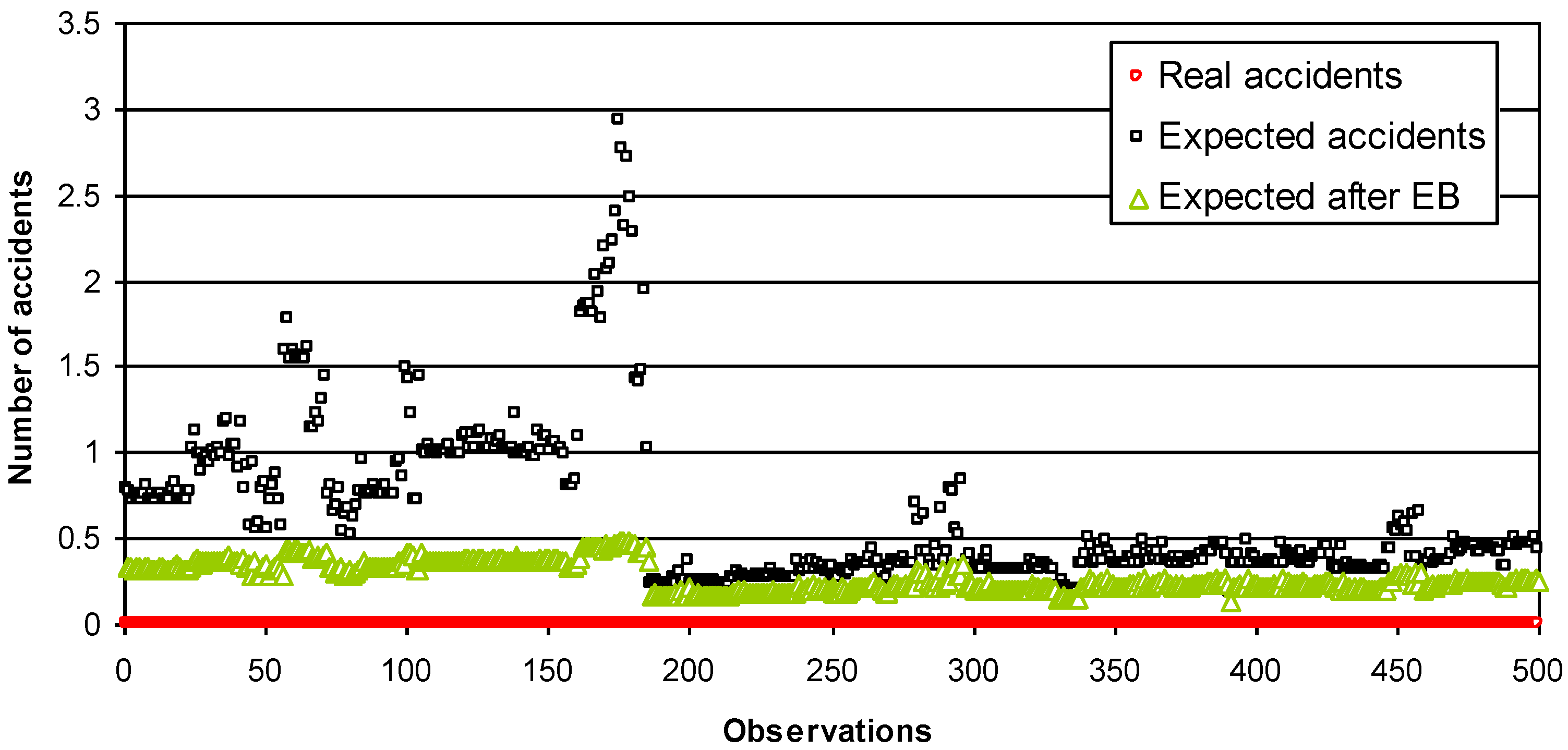
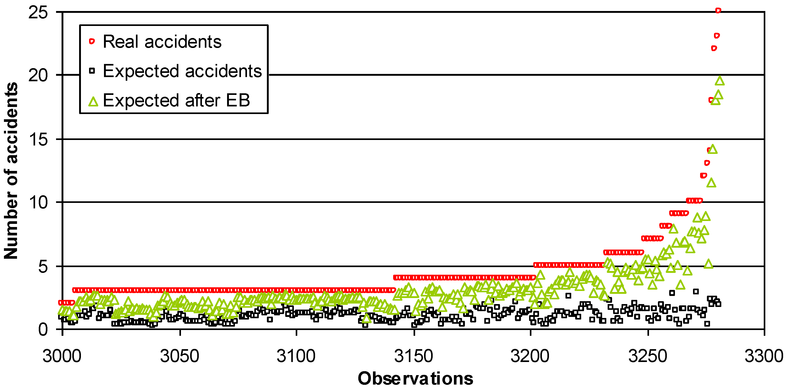
Figure 1 presents the comparison results for the road section data set of 500 m in length, including the EB method. Figure 2 and Figure 3 present the breakdown of the original data into different observation numbers.

Figure 1. Expected number of accidents comparing real number of accidents and predicted number after applying EB method (road section of 500 m).

Figure 1. Expected number of accidents comparing real number of accidents and predicted number after applying EB method (road section of 500 m).

Figure 2. Expected number of accidents comparing real number of accidents and predicted number after applying EB method (road section of 500 m)—observation 0 until 500.

Figure 2. Expected number of accidents comparing real number of accidents and predicted number after applying EB method (road section of 500 m)—observation 0 until 500.

Figure 3. Expected number of accidents comparing real number of accidents and predicted number after applying EB method (road section of 500 m)—observation 3000 until 3300.

Figure 3. Expected number of accidents comparing real number of accidents and predicted number after applying EB method (road section of 500 m)—observation 3000 until 3300.

2.4.2. Comparison of Training and Control Models

The GENMOD procedure applied on the training model (two-thirds of the data) was also applied on the control model (one-third of the data). In advance, only the parameters that were found to be significant in the training model were integrated in the control model. Table 2 presents the coefficients of the control model.

Table 2. GENMOD procedure results for the control model (one-third of the data for segments of 500 m in length).

Parameter	Estimate	Standard Error	95% Confidence Limits		X2	p
Intercept	−7.7780	0.9234	−9.6087	−5.9821	70.95	<0.0001
AADT	0.8019	0.0937	0.6197	0.9878	73.23	<0.0001
Area: South	−0.7366	0.1629	−1.0584	−0.4186	20.45	<0.0001
Area: Center	−0.8810	0.1249	−1.1274	−0.6369	49.75	<0.0001
Curvature	0.9894	0.5845	−0.1523	2.1489	2.86	0.0905
Dispersion	1.5877	0.1764	1.2701	1.9650

Table 2. GENMOD procedure results for the control model (one-third of the data for segments of 500 m in length).

Parameter	Estimate	Standard Error	95% Confidence Limits		X2	p
Intercept	−7.7780	0.9234	−9.6087	−5.9821	70.95	<0.0001
AADT	0.8019	0.0937	0.6197	0.9878	73.23	<0.0001
Area: South	−0.7366	0.1629	−1.0584	−0.4186	20.45	<0.0001
Area: Center	−0.8810	0.1249	−1.1274	−0.6369	49.75	<0.0001
Curvature	0.9894	0.5845	−0.1523	2.1489	2.86	0.0905
Dispersion	1.5877	0.1764	1.2701	1.9650

Once the estimates were calculated for the two models, the coefficients were evaluated by testing whether the model coefficient estimates for the control model fall within the confidence interval of the training model at a confidence level of 95%. For example, in the control model (Table 2), the coefficient value of the variable representing traffic volume (AADT) is 0.8019. It can be seen that this value falls within the range of 0.5883 to 0.8423 (see Table 1), meaning that the model is statistically reliable enough for predicting this variable. From the comparison of Table 1 and Table 2, it can be seen that this is true for all variables in the model, except for the variable Area: central (referring to the difference between the central area and the northern area). Here, the coefficient value −0.8810 does not fall within the confidence interval of the training model (ranging from −0.3952 to −0.7444). This means that the model is not statistically reliable enough for predicting this parameter. In addition, one may see that the variable Curvature is not significant in the control model if incorporated into the model for its lowest AIC.

2.4.3. TOST Test for Equivalence

As stated above, it is possible to compare the expected values of accidents according to the training model (two-thirds of the data) and the expected number of accidents according to the control model (one-third of the data). In a utopian world, it would be expected that the mean difference between the two models would be zero, since both models predict the same phenomenon. However, in the real world, some expected differences between the means can be predicted to range around zero. Hence, one should ask only whether the differences are within a reasonable pre-defined range. For this purpose, was used the Two One-Sided Test (TOST), (T-testing for two independent populations is not enough to address this issue because T-tests assume the data to be normally distributed,as opposed to random events, such as car accidents). In addition, T-tests are used to prove unequal results, while here we need to prove precisely equally results) which allows to verify equality for any specified range. In this study, a minimal range of −0.25 to 0.25 accidents was defined for the evaluation. If the difference between the mean (μ) values falls within the confidence interval of the difference, it indicates that the model provides similar expected predictions. Equations 2 and 3 present the test hypotheses.

H₀ = μ ˂ θ_L or μ ˃ θ_U → H₀ = μ ˂ −0.25 or μ ˃ 0.25

(2)

H₁ = θ_L ≤ μ ≤ θ_U → H₁ = −0.25 ≤ μ ≤ 0.25

(3)

where:

• θ_L, θ_U—upper and lower limit (±0.25 accident)
• μ—mean difference

Table 3 presents the TOST test results for road sections of 500 m in length. If the values in column “90% CL Mean” are between the upper range (Upper Bound) and the lower range (Lower Bound), then we accept H0 and reject H1. This means that the values of expected accidents, as calculated for the two sets of data (one-third and two-thirds), are close enough.

Table 3. TOST results for 500 m segments.

Mean	Lower Bound		90% CL Mean			Upper Bound	Assessment
−0.0548	−0.25	<	−0.0832	−0.0264	<	0.25	Equivalent

Table 3. TOST results for 500 m segments.

Mean	Lower Bound		90% CL Mean			Upper Bound	Assessment
−0.0548	−0.25	<	−0.0832	−0.0264	<	0.25	Equivalent

2.4.4. Proportions of Probabilities Comparison

It is optional to calculate estimations for the probability of the occurrence of zero accidents on road segments, one accident, two accidents, and so on. If the model is reliable enough, then we should obtain similar proportions while comparing the percentage of sections in which there were “zero accidents” in practice (using “real” world, “real” data) and the average probability of expected “zero accidents”, as calculated by the model.

Table 4 presents the calculated probabilities for the occurrence of N accidents on road sections of 500 m, as calculated from the model. This is presented for a sample of 9 segments. Each row in the table represents a specific road section of a specified length (as stated, 500 m in the current example). Each column represents the probability of the occurrence of N accidents on that section. Thus, the PO0 column represents the probability of the occurrence of zero accidents; the PO1 column represents the probability of the occurrence of one accident, and so on.

Table 4. Probabilities for the occurrence of N accidents for a sample of sections of 500 m in length.

PO0	PO1	PO2	PO3	PO4	PO5	PO6	PO7	PO8
0.610277337	0.2021285764	0.0917807833	0.0454338563	0.023412922	0.0123615103	0.0066255263	0.0035899153	0.0019608
0.60239497	0.2027937693	0.0935947405	0.0470925361	0.0246749411	0.013237001	0.0072112615	0.0039714387	0.0022048
0.606145977	0.2024918782	0.0927388184	0.0463040849	0.0240757855	0.0128165475	0.0069286689	0.0037865486	0.0020861
0.62202776	0.2009173652	0.0889710565	0.0429520422	0.0215934632	0.0111145072	0058096008	0.0030698513	0.001635
0.614599875	0.2017137307	0.090761575	0.0445217661	0.0227429164	0.0118945867	0.0063174341	0.0033919314	0.001835
0.608603762	0.2022796466	0.0921707895	0.0457865823	0.026857182	0.0125448166	0.0067473035	0.0036686911	0.0020109
0.596272816	0.2032296575	0.0949626287	0.0483751326	0.0256688671	0.0139378986	0.0076875464	0.0042864047	0.0024093
0.620124035	2.2011315691	0.0894345832	0.0433545348	0.0218860298	0.0113117258	0.0059371623	0.0031502422	0.0016850
0.622048000	0.2009150508	0.0889661124	0.0429477634	0.021590361	0.0111124209	0.0058082544	0.0030690047	0.001634

Table 4. Probabilities for the occurrence of N accidents for a sample of sections of 500 m in length.

PO0	PO1	PO2	PO3	PO4	PO5	PO6	PO7	PO8
0.610277337	0.2021285764	0.0917807833	0.0454338563	0.023412922	0.0123615103	0.0066255263	0.0035899153	0.0019608
0.60239497	0.2027937693	0.0935947405	0.0470925361	0.0246749411	0.013237001	0.0072112615	0.0039714387	0.0022048
0.606145977	0.2024918782	0.0927388184	0.0463040849	0.0240757855	0.0128165475	0.0069286689	0.0037865486	0.0020861
0.62202776	0.2009173652	0.0889710565	0.0429520422	0.0215934632	0.0111145072	0058096008	0.0030698513	0.001635
0.614599875	0.2017137307	0.090761575	0.0445217661	0.0227429164	0.0118945867	0.0063174341	0.0033919314	0.001835
0.608603762	0.2022796466	0.0921707895	0.0457865823	0.026857182	0.0125448166	0.0067473035	0.0036686911	0.0020109
0.596272816	0.2032296575	0.0949626287	0.0483751326	0.0256688671	0.0139378986	0.0076875464	0.0042864047	0.0024093
0.620124035	2.2011315691	0.0894345832	0.0433545348	0.0218860298	0.0113117258	0.0059371623	0.0031502422	0.0016850
0.622048000	0.2009150508	0.0889661124	0.0429477634	0.021590361	0.0111124209	0.0058082544	0.0030690047	0.001634

Table 5 presents the mean of columns PO0 and PO1 (the average probability for zero accidents, the average probability of one accident, and so on), as presented in Table 4.

Table 5. Mean probabilities for the occurrence of zero and one accidents on 500 m segments.

Variable	N	Mean	Std Dev	Minimum	Maximum
PO0	2188	0.6582303	0.1082179	0.3312983	0.8639541
PO1	2188	0.1837504	0.0245488	0.1115330	0.2043939

Table 5. Mean probabilities for the occurrence of zero and one accidents on 500 m segments.

Variable	N	Mean	Std Dev	Minimum	Maximum
PO0	2188	0.6582303	0.1082179	0.3312983	0.8639541
PO1	2188	0.1837504	0.0245488	0.1115330	0.2043939

Table 6. Real data accident proportions for N accidents (road segments of 500 m in length).

AccCNT
AccCNT	Frequency	Percent	Cumulative Frequency	Cumulative Percent
0	1441	65.86	1441	65.86
1	397	18.14	1838	84.00
2	170	7.77	2008	91.77
3	87	3.98	2095	95.75
4	37	1.69	2132	97.44
5	25	1.14	2157	98.58
6	12	0.55	2169	99.13
7	5	0.23	2174	99.36
8	2	0.09	2176	99.45
9	4	0.18	2180	99.63
10	3	0.14	2183	99.77
13	1	0.05	2184	99.82
14	1	0.05	2185	99.86
18	1	0.05	2186	99.91
23	1	0.05	2187	99.95
25	1	0.05	2188	100.00

Table 6. Real data accident proportions for N accidents (road segments of 500 m in length).

AccCNT
AccCNT	Frequency	Percent	Cumulative Frequency	Cumulative Percent
0	1441	65.86	1441	65.86
1	397	18.14	1838	84.00
2	170	7.77	2008	91.77
3	87	3.98	2095	95.75
4	37	1.69	2132	97.44
5	25	1.14	2157	98.58
6	12	0.55	2169	99.13
7	5	0.23	2174	99.36
8	2	0.09	2176	99.45
9	4	0.18	2180	99.63
10	3	0.14	2183	99.77
13	1	0.05	2184	99.82
14	1	0.05	2185	99.86
18	1	0.05	2186	99.91
23	1	0.05	2187	99.95
25	1	0.05	2188	100.00

The “PO1” column in Table 5, presents the model calculated probability for one accident occurrence for all database segments. The mean value was 0.1837 (18.37%). This value is very close to the value of 18.14%, which is the value of the actual proportion of segments that had only one accident on them, in the 500 m length database during the study period (see Table 6 at column AccCNT = 1).

2.4.5. Training Model (Two-Thirds Data) and Full Control Model (One-Third Data) Comparison

A new model based on one-third of the data was constructed to serve as the “full control model” due to its use of all existing parameters in the data set, as opposed to the previous “control” models in which only the significant parameters were combined. The comparison between the two models provided an additional control and enabled an assurance test on the results of the training model (two-thirds of the data) at various levels. It also allowed for validation of the model type (data distribution aspect). Thus, it served as an additional control for the parameters obtained from the significant model, as well as a control for the estimates obtained from the model.

3. Results, Analysis and Discussion

3.1. Optimal Models

The study shows that the shorter segment data sets tested (lengths of 500 and 750 m) yielded the most stable models. This means that recommendations can be made concerning investments in the infrastructure and enforcement for short sections, as opposed to the prevailing attitude of improving relatively long sections of the road network.

Equation (4) represents the expected rate of road accidents (μ) for highway sections of 500 m in length:

μ = e^{−7.091 + 0.714 × AADT_Log + (−0.678) × Region1 + (0.569) × Region3 + (1.594) × CurvePrm3}

(4)

Equation (5) represents the expected rate of road accidents (μ) for highway sections of 750 m in length:

μ = e^{−5.9688 + 0.6420 × AADT_Log + (−0.7316) × Region1 + (0.5483) × Region3 + (1.0741) × CurvePrm3}

(5)

where: AADT_Log—annual average daily traffic after it has been transformed using a natural logarithm. Region—while Region1 = the southern area; Region 2 = the northern area; and Region 3 = the central area, the model compares and analyzes the northern region in relation to the two other regions. Thus, for a section located in Region 2, the value that will be placed at variables Region 3 and Region 1 will be 0. Curvature—segment curvature. Calculated by the sum of the differences between the nearest H, divided by segment length (H in red: the vertical distance between the parabola tip and the line segment connecting the strands—appears as a dotted line), as specified in Equation (6) and Figure 4.

(6)

Figure 4. Curvature calculation.

Figure 4. Curvature calculation.

After calculating the expected accident rates, the EB method was applied in order to further improve the model.

3.2. Model Parameters

Of all the parameters that were examined in this study, the curvature of the road section, the region, and the traffic volume were found to be the most significant in terms of affecting accidents. Due to its high expected accident rates the northern region was designated for special observation and was divided into sub-regions that were analyzed separately.

3.2.1. Curvature

The curvature and traffic volume findings match [18] study. However, unlike Miaou’s research, which identified a relationship between curvature and the accident rate only for large trucks, the current study addressed all types of vehicles and carried out rules for the data using the EB method. The traffic volume (aadt log) parameter was also found to be meaningful. This finding matches other studies, including [5,6,10,27].

3.2.2. Region

The third variable found to be significant was the region. In Israel, this variable is compatible with the major divisions of the “periphery” (North and South) and the central area (Tel Aviv metropolis). All of the analyses consistently showed the highest expected accident rates to be in the northern area and particularly in the Western Upper Galilee. Therefore, the results concerning this variable should be further analyzed and checked in several aspects.

The region variable was analyzed during the first step of building the models. This parameter appeared to be significant in all four models, as constructed for various lengths of road sections. In all four models, the accident rate for the northern part of Israel was expected to be higher (approximately twice as high) than the expected rate of accidents for the central and southern parts of Israel.

The second regional analysis examined the statistical differences between the northern, southern, and central regions. This analysis aimed to examine the statistical differences between the regions, and to learn whether a particular area will depict more or less accidents, regardless of the volume of traffic. The data set was divided into several traffic volume ranges: “low”, “medium-low”, “medium-high”, and “high”. Due to the need to maintain balanced groups for the statistical analysis, only groups with sufficient samples were analyzed. In practice, only the “medium–low” group (5000 to 15,000 vehicles per road section) and the “medium–high” group (15,000 to 30,000 vehicles per road section) were analyzed.

In this analysis, the trends were similar at road lengths of 500 and 750 m for the “medium–low” and the “medium–high” road sections, with the expected accident rate in the northern region greater than expected in the southern region and the expected accident rate in the northern region greater than expected in the central region. These trends are also consistent with the results obtained in the previous regions analysis performed on the training model (the expected accident rate at north is higher than expected at the central and southern regions.

When comparing the predicted accident rates of the central and southern regions, different relations were found:

(1) At “medium-low” traffic volumes, the expected accident rates in the central region were greater than expected in the southern region. This may be explained by the fact that in the south, despite dealing with accidents at so-called medium-low traffic volumes, the traffic volumes are truly lower, meaning that the roads actually carry very sparse traffic. The logic is simple: Given that very few vehicles (low range value) are present, the probability for accidents drastically decreases in this region, as compared to the central region, where vehicles are present at the higher end of the “medium-low” traffic volume range.

(2) At “medium-high” traffic volumes, the expected accident rates in the southern region were greater than expected in the central region. The presumed explanation is that as traffic increases, it is more vulnerable to the effects of the infrastructure quality, such as unregulated intersections that flow directly into the highways, fewer lanes, and lack of lane separation. As the infrastructure in the southern region was much poorer than in the central region at the time of the study, it affected the accident sensitivity rates.

The third aspect of the regional analysis was the interaction analysis. Unlike the previous analyses, here, the traffic volume serves as a parameter. Thus, there is difference in division of the traffic volume thresholds. This was carried out by partitioning the segments into three groups: “low” traffic volume, characterized by values ranging from 0 to 10,766; “medium” traffic volume, characterized by values ranging between 10,767 and 20,033; and “high” traffic volume, characterized by values over 20,033.

An interaction between the region and the traffic volume variables was found for both data sets examined. This means that the effect of traffic volume on the expected rate of accidents is not uniform and depends on the region as well (see Table 7). The interaction analysis findings match the results of the first and second analyses. All other interactions such as region and curvature, and region and slope were not found significant, and thus, were not further examined as were the AADT and region. The significance test was carried out by comparing AIC value of “Null model” (The “Null Model” containing the variables: curvature, area and volume of traffic without variable representing interaction), with three other models that contained also interactions as parameters.

The anomaly as depicted at Table 7 where the expected results for “Medium traffic” is higher than for the “High” in the southern area is intriguing indeed. This is biased due to the division of the traffic groups. The maximum daily traffic in the south area was 23,000. This further implies that the “High traffic” group almost does non exit in this area. Only 72 records were found in the south area for this group and this actually biased the results.

Table 7. Interactions—number of expected accidents divided into regions (Section lengths of 500 m and 750 m).

Data Set	AADT	Area	Expected Number of Accidents
500 m	Low	south	0.51
	medium	south	1.51
	High	south	1.19
	Low	north	1.64
	medium	north	2.29
	High	north	4.10
	Low	center	1.32
	medium	center	1.05
	High	center	2.38
750 m	Low	south	0.74
	medium	south	2.3
	High	south	1.89
	Low	north	2.22
	medium	north	3.55
	High	north	5.45
	Low	center	2.06
	medium	center	1.41
	High	center	3.74

Table 7. Interactions—number of expected accidents divided into regions (Section lengths of 500 m and 750 m).

Data Set	AADT	Area	Expected Number of Accidents
500 m	Low	south	0.51
	medium	south	1.51
	High	south	1.19
	Low	north	1.64
	medium	north	2.29
	High	north	4.10
	Low	center	1.32
	medium	center	1.05
	High	center	2.38
750 m	Low	south	0.74
	medium	south	2.3
	High	south	1.89
	Low	north	2.22
	medium	north	3.55
	High	north	5.45
	Low	center	2.06
	medium	center	1.41
	High	center	3.74

In the last analysis of the region variable, the northern area was designated for special observation due to its high expected accident rates. The area was divided into eight sub-regions, and the analysis was performed on the full accident data (without dividing into 2/3 and 1/3). One sub area, “Golan Heights”, was eliminated from the analysis due to low number of accidents events during the research period. The Linear Step-up procedure was applied in order for detecting false discovery rate. The analysis results showed significant high expected accident rates in the Western Upper Galilee sub-region. According to this finding, it is recommended that a range of practical activities be carried out, from improvement of infrastructure to education and advocacy.

3.2.3. Speed

Interestingly, the speed variable was not determined to be significant by this study. This conclusion is in agreement with other published studies, such as [15], which found that the accident rate rose in accordance with increasing speed on non-major roads. Yet, on main roads, it was found that the path width, the density of nodes, and traffic had higher correlations with the accident rate.

The speed parameter, as integrated into this study, was only estimated. In order to be able to assess this parameter more accurately in future studies, it is necessary to acquire and integrate more accurate speed data, perhaps even from different points in time, such as day and night, weekdays and weekends, and so on.

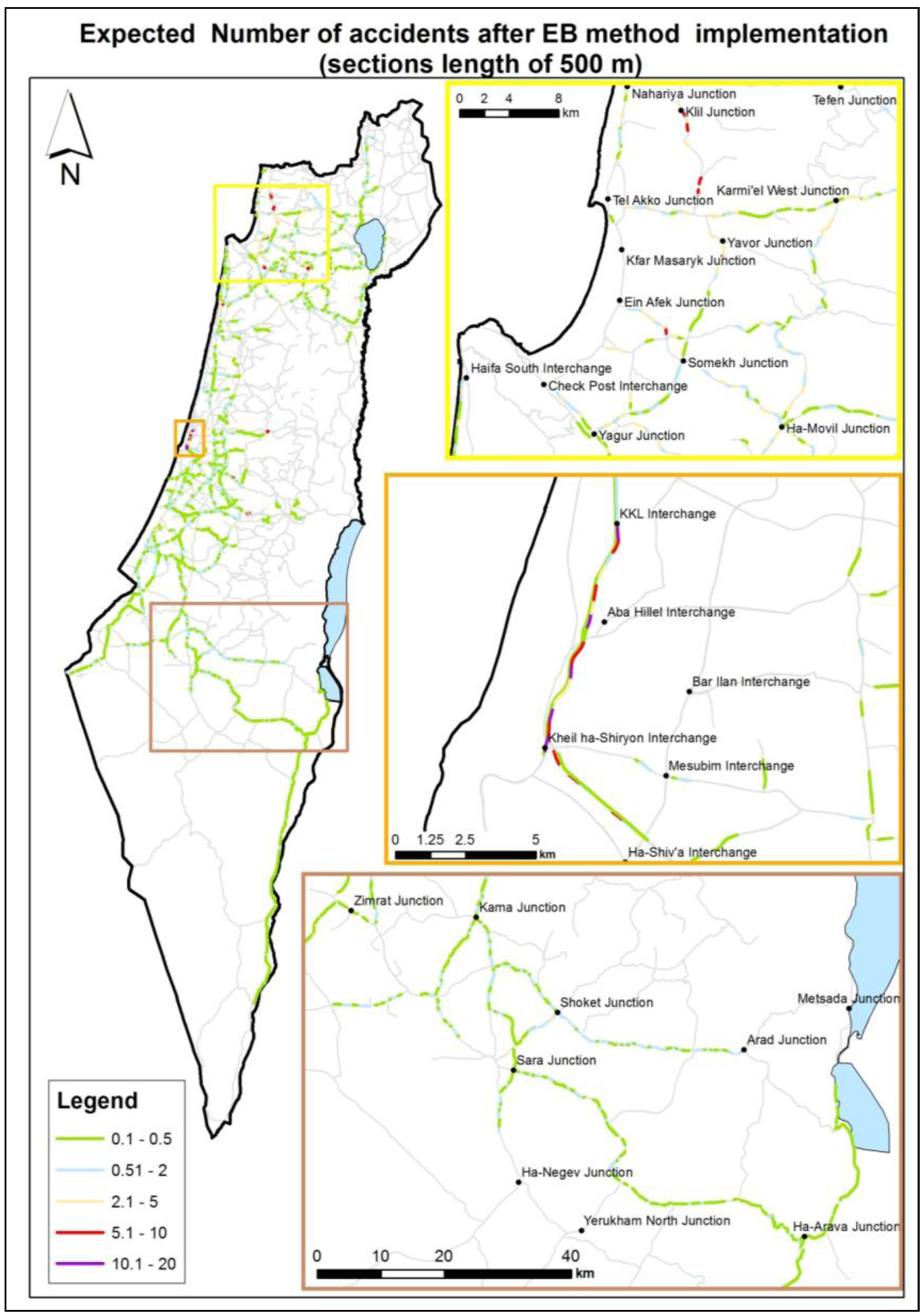
Figure 5. Expected number of accidents (road sections at length of 500 m).

Figure 5. Expected number of accidents (road sections at length of 500 m).

3.2.4. Solar Angle (Sun Glare)

Each accident was positioned using ESRI ArcGIS software address matching process. After the location was found the azimuth and slope of the car were calculated based on Digital Elevation Model.

The sun glare value was calculated for each accident using a batch of equations migrated to MS Access software. Due to the high uncertainty of the direction of the car during the accident (upstream or downstream) many of the resulted declination were incorrect. This affected the integrity of the sun glare values. Thus the sun glare was taken out as a parameter in this research but it is recommended to use it once we have accurate and valid data.

3.2.5. Prediction Maps

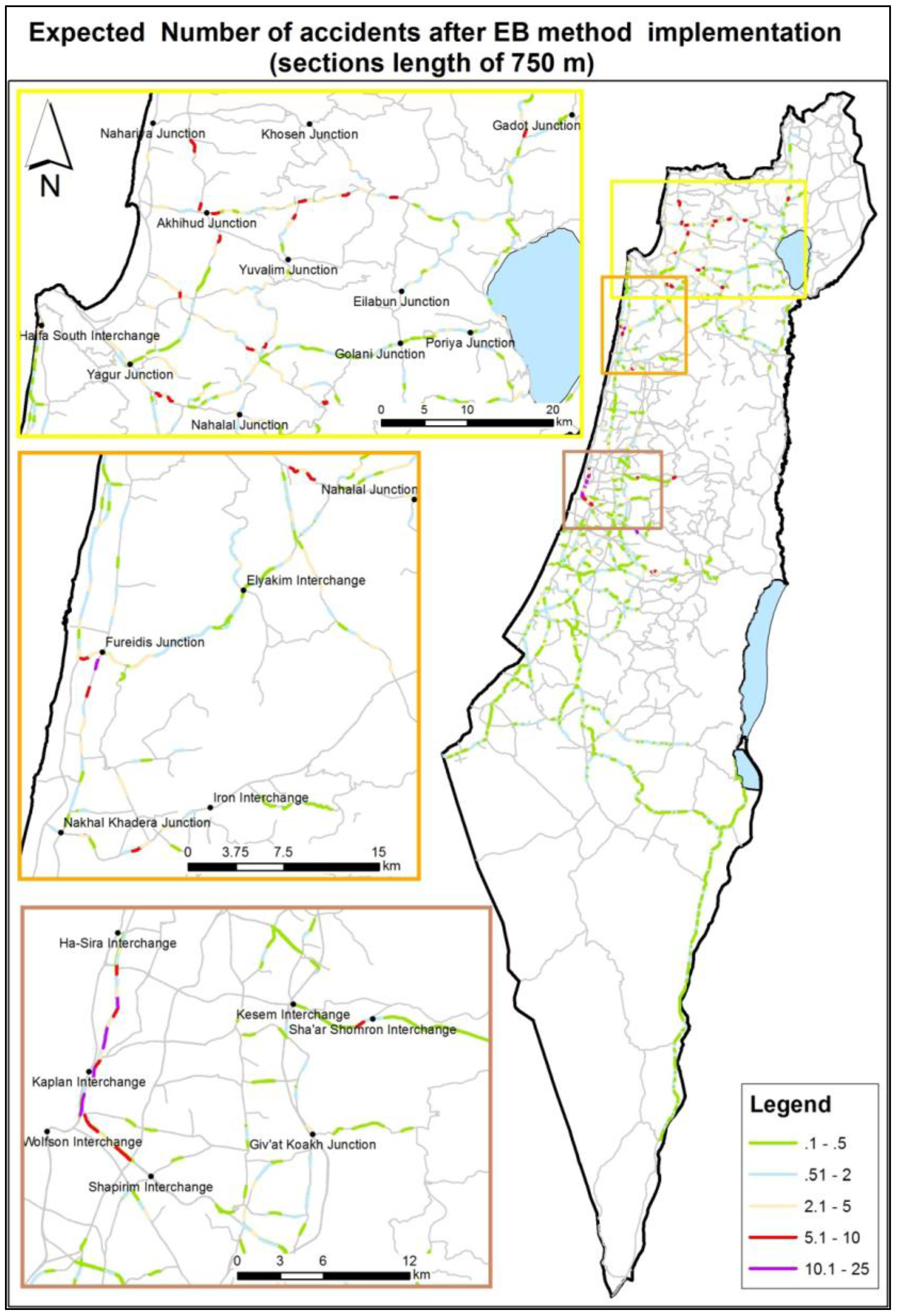
Figure 5 and Figure 6 present some of the final research outputs. The maps display the expected number of accidents on road sections after the correction procedure of EB. The amplitude of the expected number of accidents is depicted by a color palette, ranging from green, which represents road sections with a low number of expected accidents, to red and purple, representing sections with high rates of expected accidents. It should be emphasized that when positioning the accidents on the road sections, the direction was selected according to CBS data despite its lack of precision [23]. The rationale here was that in terms of physical road parameters, it can be assumed that dangerous road sections from one direction would also be dangerous on the opposite lane.

Figure 6. Expected number of accidents (road sections at length of 750 m).

Figure 6. Expected number of accidents (road sections at length of 750 m).

4. Reproducibility and Opportunities for Further Study

This paper described the development of GIS-based prediction models for the assessment of traffic accidents in highway segments, using spatial and traffic-based parameters. The findings of this research constitute a basis and a starting point for other varied studies in the field of road safety. First and foremost it is proposed to examine the quality of the model on accident data of future years. This model can also be implanted in other countries/regions and in addition, at various segmentation e.g., roadway functional classes, vehicle configurations, types of crashes (e.g., those involving drunk drivers), and crash severity levels (e.g., fatal, injury, and non-injury events). It is also suggested to perform spatial autocorrelation, looking into influence of nearby segments.

According to the research finding, the analyses of the “region” variable produced very distinct and alarming high expected accident rates in the northern region. This is distinct especially in the western Upper Galilee sub-region. Also remarkably distinct were the substantiated findings of interaction between the “region” and the “traffic volume” variables. The conclusion is that the effect of “traffic volume” on the expected rate of accidents is not uniform and depends on the region as well. Thus, suggested is to investigate the “region” and the “sub region” variables more closely while associating: environmental, socioeconomic and economic variables to the model. Among these are: infrastructure investments, shoulders width, lanes separation, number of lanes, etc.

The speed parameter, as integrated into this study, was only estimated. In order to assess this parameter more accurately in future studies, it is necessary to acquire and integrate more accurate speed data. Hence, suggested here is getting speed data from navigation applications and traffic reports based on user’s community and to analyze speed effect at different times (day and night, weekdays and weekends, and so on).

We believe that the Scholl width and number of lanes are significant variables of the existence of road accidents. These data is not collected currently at continuously and accurately as it should. Accurate data for both these variables will outcome with more reliable results and models. In addition, accident orientation data which is considered as not reliable at this study is also recommended to integrate while placing accident at its occurrence site in other studies.

5. Conclusions

This paper described the development of a GIS-based prediction model for the assessment of traffic accidents in highway segments, using spatial and traffic-based parameters.

The most significant and practical “revelation” in this study is that the short road sections yielded the most stable models. This allows aiming the treatments on short sections of the road as a way to save resources and potentially gain maximum benefit at minimum investment. The ability to narrow down the high-risk areas to specific road sections also enable to focus the police (and other) enforcement teams at those sections in order for save life. The models were improved by using the Empirical Bayes method, which increased the accuracy of the assessment by taking into account historical data and correcting the biases from the “regression to the mean” phenomenon. In addition, it was found that the most significant variables affecting accident rates were: curvature of the road section, the region, and the traffic volume. In addition, an interaction between the region and the traffic volume variables was found. This means that the influence of traffic volume on the expected rates of accidents is not uniform and depends on the region as well. Investigating this issue more profoundly will probably raise some very interesting finding. The categorization of the data set according to road sections of different but equal lengths allowed “neutralizing” the “segment length” parameter, which in many studies was found to be a significant parameter in the model.

This study confirms, once again, the power and benefits of using Geographic Information Systems (GIS) in the field of road safety (GIS-T). This approach allows for displaying and examining the data in “real” space (i.e., the physical location where the events occur), iteration, and performing complex statistical-spatial analysis in a relatively simple manner.

References

1. Page, Y. A statistical model to compare road mortality in OECD countries. Accid. Anal. Prev. 2001, 33, 371–385. [Google Scholar] [CrossRef]
2. Miaou, S.P.; Song, J.J.; Mallick, B.K. Roadway traffic crash mapping: A space-time modeling approach. J. Transp. Stat. 2003, 6, 33–57. [Google Scholar]
3. Peled, A. Detection Urban Safety Issues Using Geographic Information System (GIS); Institute of Transportation Studies: Jerusalem, Israel, 1996. [Google Scholar]
4. Hakim, S.; Shefer, D.; Hakkert, S.; Hocherman, I. A critical review of macro models for road accidents. Accid. Anal. Prev. 1991, 23, 379–400. [Google Scholar] [CrossRef]
5. Levine, N.; Kim, K.; Nitz, L. Spatial analysis of Honolulu motor vehicle crashes: I. Spatial patterns. Accid. Anal. Prev. 1995, 27, 663–674. [Google Scholar] [CrossRef]
6. Levine, N.; Kim, K.; Nitz, L. Spatial analysis of Honolulu motor vehicle crashes: II. Zonal generators. Accid. Anal. Prev. 1995, 27, 675–685. [Google Scholar]
7. Summala, H. Accident risk and driver behavior. Saf. Sci. 1996, 22, 103–117. [Google Scholar] [CrossRef]
8. Jones, A.P.; Langford, I.H.; Bentham, G. The application of K-function analysis to the geographical distribution of road traffic accident outcomes in Norfolk, England. Soc. Sci. Med. 1996, 42, 879–885. [Google Scholar] [CrossRef]
9. Beenstock, M.; Goldin, A.; Gafni-Sri, D. The Relationship between Traffic Enforcement and Road Accidents: Statistical Analysis; Office of the Chief Scientist, Ministry of Public Security: Jerusalem, Israel, 1998. [Google Scholar]
10. Oppe, S. Development of traffic and traffic safety: Global trends and incidental fluctuations. Accid. Anal. Prev. 1991, 23, 413–422. [Google Scholar] [CrossRef]
11. Ng, K.S.; Hung, W.T.; Wong, W.G. An algorithm for assessing the risk of traffic accident. J. Saf. Res. 2002, 33, 387–410. [Google Scholar] [CrossRef]
12. Schneider, R.J.; Ryznar, R.M.; Khattak, J.A. An accident waiting to happen: A spatial approach to proactive pedestrian planning. Accid. Anal. Prev. 2004, 36, 193–211. [Google Scholar] [CrossRef]
13. Qin, X.; Ivan, J.N.; Ravishanker, N.; Liu, J. Hierarchical Bayesian estimation of safety performance functions for two-lane highways using Markov chain Monte Carlo modeling. J. Transp. Eng. 2005, 131, 345–351. [Google Scholar] [CrossRef]
14. Sabel, C.E.; Kingham, S.; Nicholson, A.; Bartie, P. Road Traffic Accident Simulation Modelling—A Kernel Estimation Approach; Otago University: Dunedin, New Zealand, 2005. [Google Scholar]
15. Aarts, L.; van Schagen, I. Driving speed and the risk of road crashes: A review. Accid. Anal. Prev. 2006, 38, 215–224. [Google Scholar] [CrossRef]
16. Song, J.J.; Ghosh, M.; Miaou, S.; Mallick, B. Bayesian multivariate spatial models for roadway traffic crash mapping. J. Multivar. Anal. 2006, 97, 246–273. [Google Scholar] [CrossRef]
17. Miaou, S.P.; Lum, H. Modeling vehicle accidents and highway geometric design relationships. Accid. Anal. Prev. 1993, 25, 689–709. [Google Scholar] [CrossRef]
18. Miaou, S.P. The relationship between truck accidents and geometric design of road sections: Poisson versus negative binomial regressions. Accid. Anal. Prev. 1994, 26, 471–482. [Google Scholar] [CrossRef]
19. Baruya, A. Working Paper: A Review of Speed-Accident Relationship on European Roads. Master’s Thesis, Transport Research Laboratory, Wokingham, UK, August 1997. [Google Scholar]
20. Aguero, V.J.; Jovanis, P.P. Analysis of road crash frequency with spatial models. Transp. Res. Rec. 2008, 2061, 55–63. [Google Scholar] [CrossRef]
21. Peled, A.; Hakkert, A.S. A PC-oriented GIS application for road safety analysis and management. Traffic Eng. Control 1993, 34, 355–361. [Google Scholar]
22. Peled, A.; Haj-Yehia, B.; Hakkert, A.S. ArcInfo-Based Geographical Information System for Road Safety Analysis and Improvement. Available online: http://proceedings.esri.com/library/userconf/proc96/to50/pap005/p5.htm (accessed on 13 August 2013).
23. The Central Bureau of Statistics. Road Accidents with Injuries in 2007 Part II: Accidents on—Rural Roads; The Central Bureau of Statistics: Jerusalem, Israel, 2007.
24. Nelder, J.A.; Wedderburn, R.W.M. Generalized linear models. J. Royal Stat. Soc. Ser. A 1972, 135, 370–384. [Google Scholar] [CrossRef]
25. Hauer, E. Empirical bayes approach to the estimation of “unsafety”: The multivariate regression method. Accid. Anal. Prev. 1992, 24, 457–477. [Google Scholar] [CrossRef]
26. Sayed, T.; Rodriguez, F. Accident prediction models for urban unsignalized intersections in British Columbia. Transp. Res. Rec. 1999, 1665, 93–99. [Google Scholar]
27. Hauer, E. Overdispersion in modeling accidents on road sections and in Empirical Bayes estimation. Accid. Anal. Prev. 2001, 33, 799–808. [Google Scholar] [CrossRef]