1. Introduction
The evolution of urban areas has historically been closely intertwined with the development of transportation infrastructure, with public transport (PT) playing a fundamental role in shaping sustainable and accessible cities [
1,
2]. In rapidly urbanizing metropolitan regions, effective public transit systems substantially enhance connectivity, stimulate economic activity, and foster social integration, while simultaneously mitigating traffic congestion and environmental impacts [
1,
3]. Cities in the Mediterranean region, and particularly those characterized by dense populations, complex geography, and intense urban development patterns, are increasingly reliant on metro networks and complementary PT modes to address growing mobility demands [
4,
5].
Contemporary urban transportation planning faces unprecedented challenges as cities grapple with sustainability imperatives, social equity concerns, and technological transformation [
3,
6]. The urgency for change in mobility planning has been widely recognized at the international level, with scholars emphasizing the need for context-adapted approaches that can facilitate rapid transitions toward sustainable transportation systems [
3]. However, there remains no general agreement on the best strategies to pursue such transformative change, particularly in complex metropolitan environments where diverse socioeconomic populations interact with varied transportation infrastructure [
3].
Transportation accessibility has emerged as a critical lens through which to understand urban mobility patterns and their implications for social inclusion, referring to the extent to which individuals can reach desired destinations using public transportation and encompassing both the physical availability of services and the socioeconomic barriers that may limit access [
7,
8].
The measurement of public transport accessibility has evolved considerably over the past three decades. Traditional approaches focused primarily on proximity-based measures, calculating distances or travel times to transit stations [
7]. However, contemporary accessibility research emphasizes the importance of considering multiple factors including service frequency, connectivity, travel costs, and the spatial distribution of opportunities [
9,
10,
11,
12]. Advanced accessibility measures now incorporate considerations of service reliability, transfer requirements, and the temporal variability of service provision [
13,
14].
The integration of Geographic Information Systems (GISs) with advanced statistical and spatial modeling techniques has markedly improved researchers’ ability to analyze spatial patterns in transportation systems [
15,
16]. This technological advancement enables detailed investigations into how geographic accessibility and resident profiles interact to shape transport demand, providing insights that were previously difficult to obtain through traditional analytical approaches [
16,
17]. Prior research has also underscored the critical role of socioeconomic and demographic characteristics in shaping travel behaviors and transit use [
18,
19].
Network-based visualization approaches, in particular, provide detailed and accurate ways of estimating accessibilities in urban environments, allowing researchers to model changes in accessibility with high spatial precision [
17,
20].
Catchment area analysis has become a standard approach for understanding the spatial influence of transit stations [
21,
22]. Traditional methods often relied on simple buffer zones around stations, but contemporary research increasingly employs more sophisticated approaches that account for actual walking routes, topography, and barriers to pedestrian movement [
21,
23]. The use of isochrone-based catchment areas, which delineate areas accessible within specific travel times, provides more realistic representations of station accessibility than simple distance-based measures [
22].
The application of Geographically Weighted Regression (GWR) and its variants has revolutionized the study of spatial relationships in transportation research [
16,
24,
25]. Unlike traditional global regression models that assume spatial stationarity, GWR allows for the exploration of local variations in relationships between variables, providing insights into how the factors influencing transit ridership may vary across different urban contexts [
16,
26].
Recent applications of GWR in transit research have demonstrated its superior performance compared to traditional Ordinary Least Squares (OLS) approaches [
17,
26,
27]. Studies examining public transport demand have found that GWR models consistently achieve higher explanatory power and provide more nuanced insights into the spatial heterogeneity of travel behavior [
16,
17]. The method has proven particularly valuable for identifying areas where standard relationships between socioeconomic factors and transit use break down, highlighting locations that may require targeted policy interventions [
24,
26].
Principal Component Analysis (PCA) has emerged as a valuable complement to spatial regression techniques, particularly in contexts where large numbers of potentially correlated explanatory variables are available [
17,
28]. By reducing dimensionality while retaining explanatory power, PCA enables researchers to identify underlying latent factors that influence travel behavior [
28]. This approach has proven particularly useful in studies examining the relationship between socioeconomic characteristics and mode choice, where multiple correlated variables may represent similar underlying constructs [
28,
29].
Although previous studies have shown that metro and public transport demand is influenced by socioeconomic characteristics, accessibility conditions, and spatial structure, evidence remains uneven across metropolitan contexts. Mediterranean and Southeastern European metro systems, including Athens, have received less attention than the much larger body of work on North American and East Asian systems, despite their dense urban form, strong center-periphery contrasts, and uneven public transport accessibility. At the same time, many ridership studies rely either on global models that estimate average relationships across the full network or on local spatial models that reveal spatial heterogeneity, without explicitly comparing what each approach contributes under the same station-level dataset [
30].
A further challenge concerns the interpretation of large sets of census indicators. When many socioeconomic variables are available, analysis is often hindered by multicollinearity and by the absence of a parsimonious reduction step that can support interpretation without discarding the broader social context of station catchments.
The Athens Metro provides a relevant case for examining these issues because station demand is shaped not only by network centrality and interchange functions, but also by the socioeconomic composition of surrounding accessible areas. This is particularly important in a metropolitan region where peripheral and suburban areas may face greater car dependence, weaker feeder accessibility, and different commuting patterns than central areas. Understanding these differences can support more targeted, equity-oriented public transport planning.
Against this background, this study applies an integrated GIS and spatial modeling workflow to Athens Metro station catchments. The analysis combines network-based 10 min walking isochrones, month-specific OLS models, GWR local-coefficient diagnostics, and PCA in order to distinguish network-wide average relationships from place-specific variations and to reduce the dimensionality of correlated census indicators. The study addresses three questions: (a) Which socioeconomic characteristics are associated with metro ridership across Athens station catchments? (b) How do these relationships vary spatially, and what do such variations suggest about transport accessibility and equity, with equity interpreted here descriptively as the uneven distribution of metro-related accessibility benefits across areas with different socioeconomic profiles? (c) How can a combined global-local analytical workflow improve interpretation when numerous, potentially correlated socioeconomic indicators are available?
2. Materials and Methods
2.1. Study Area and Data
The study focuses on the Attica region of Greece, specifically areas served by the Athens Metro network, which forms the backbone of the region’s public transport system. Attica’s complex urban fabric, marked socioeconomic contrasts, and significant share of Greece’s urban population make it a compelling case for investigating socioeconomic and spatial factors influencing metro ridership patterns. The selection of 2021 provides a consistent annual record of ridership and socioeconomic conditions for all stations under study. Although residual post-pandemic effects cannot be excluded, using the full year allows seasonal variation to be examined within a common temporal framework.
Monthly ridership data for all metro stations were obtained from OASA through the national open data portal (
data.gov.gr), consistent with contemporary trends toward open government data [
31], while socioeconomic data comprising 72 indicators were retrieved from the Hellenic Statistical Authority (ELSTAT), selected based on established frameworks in accessibility research [
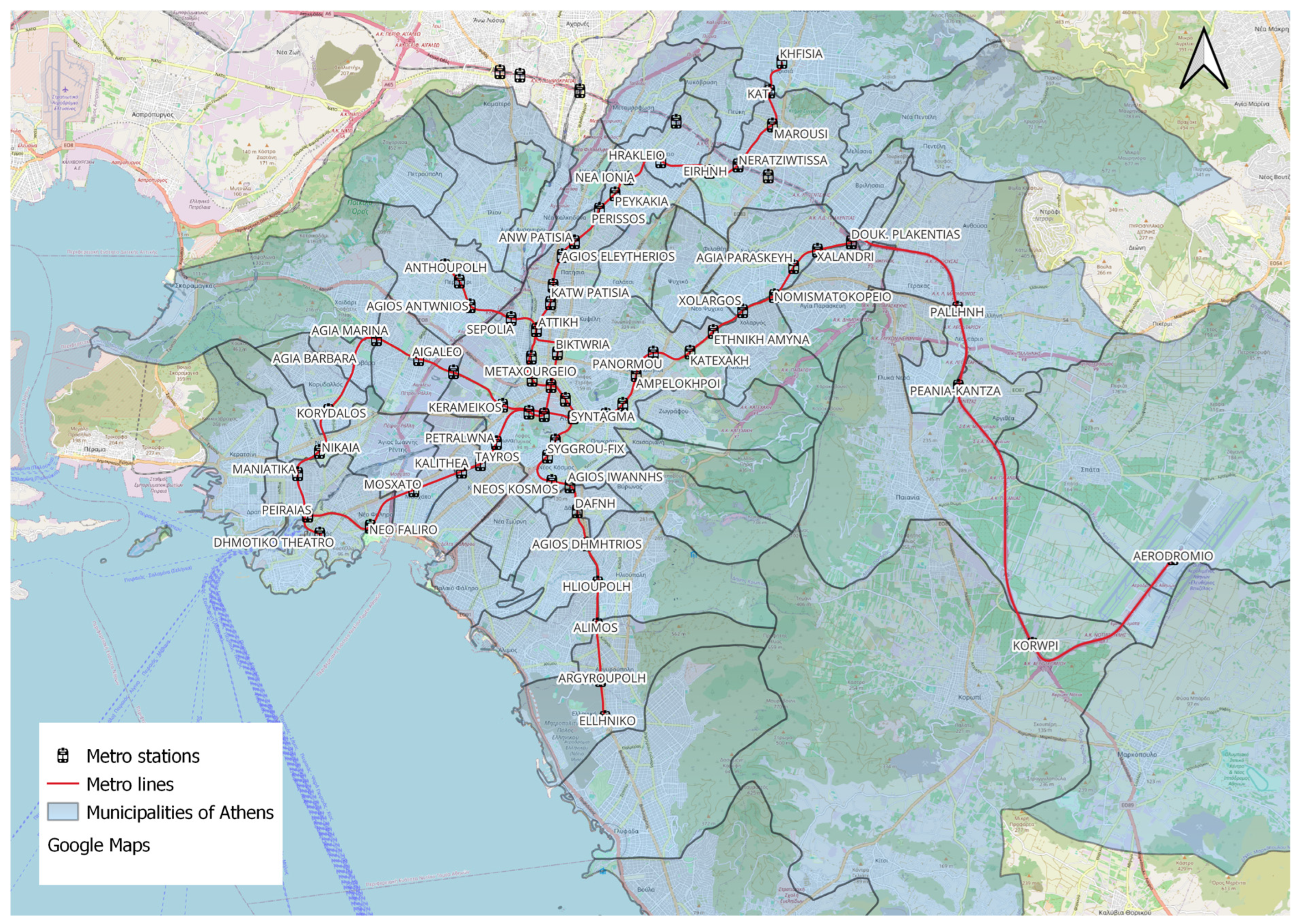
7]. In this study, ridership is operationalized as the aggregate monthly station-level usage measure available in the OASA dataset. The available data do not distinguish boarding from alighting movements, nor do they separate users by fare product (e.g., commuter passes versus single tickets). The analysis therefore focuses on overall station usage rather than on specific trip purposes or user categories. All metro stations were visualized and imported into QGIS 3.28. The study area, along with the metro stations used in this study, is shown in
Figure 1, while the resulting catchment areas are shown in
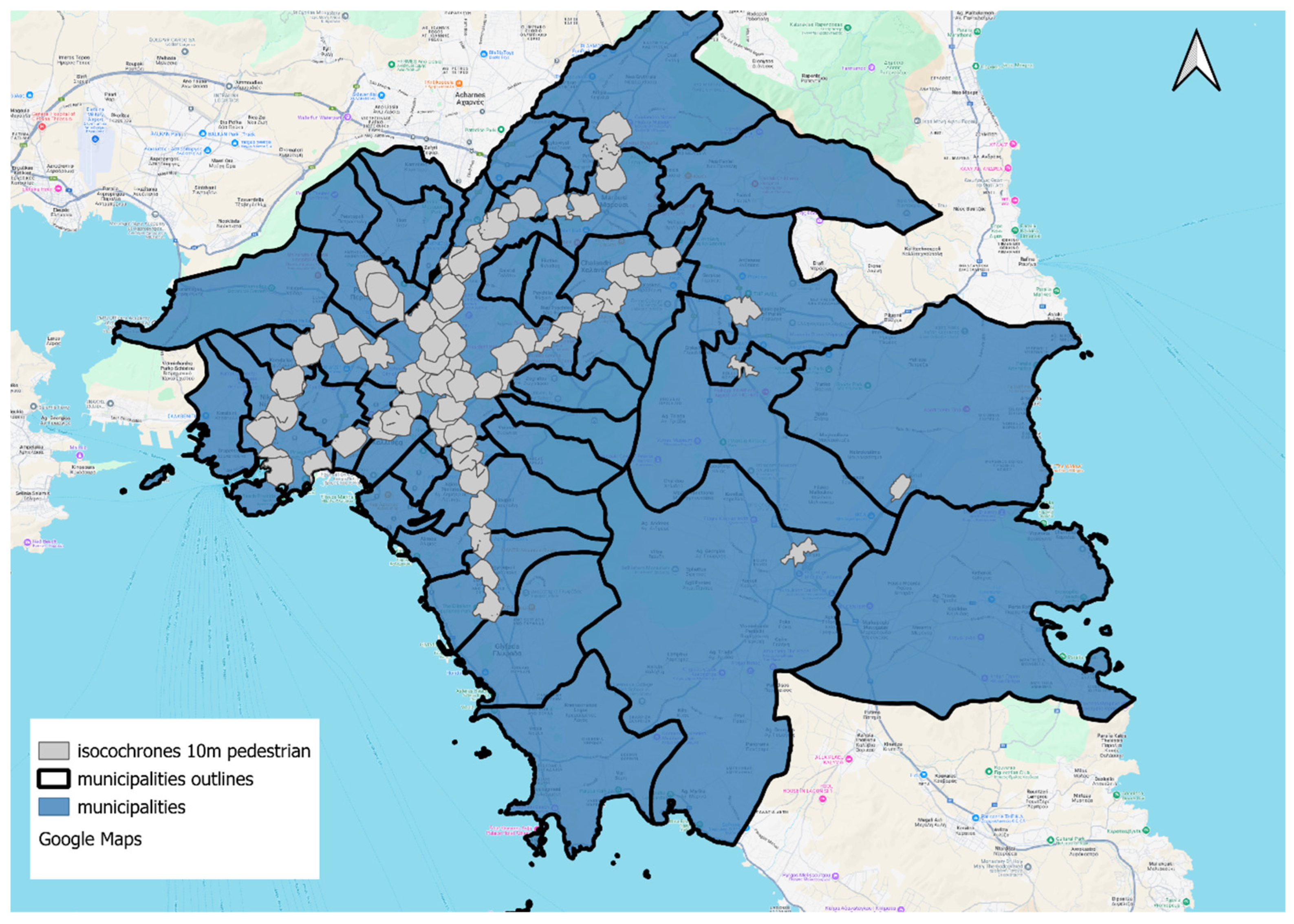
Figure 2.
Around each station, catchment areas were created representing 10 min walking distances, consistent with international transit accessibility standards [
16,
32], serving as analysis zones for spatial aggregation of demographic variables. Spatial intersection operations matched stations with socioeconomic indicators using area-weighted interpolation methods validated in transit accessibility studies [
33]. This created a unified geodatabase containing monthly ridership volumes and associated socioeconomic descriptors for each station.
The 10 min walking isochrones were used to represent the potential pedestrian accessibility area of each metro station. In dense parts of the Athens Metro network, especially around central stations, these catchments may overlap because residents may be within walking distance of more than one station. Therefore, the catchments should be interpreted as station-specific accessibility zones rather than as mutually exclusive service areas. No Thiessen/Voronoi-based partitioning was applied in the present analysis. As a result, some socioeconomic attributes may be represented in more than one station catchment where walking-access areas overlap. This issue is addressed as a methodological limitation, and the regression results are interpreted as exploratory station–catchment associations rather than as effects derived from exclusive population allocation.
The socioeconomic variables included in the analysis derive from census-based indicators aggregated at the station catchment level. Variables such as “households with parking spaces” refer to the absolute number of households within each 10 min walking isochrone exhibiting the respective characteristic, rather than density measures. Accordingly, the variables represent counts of socioeconomic attributes within each catchment area.
2.2. Integrated Statistical Modeling Approach
Bivariate correlation analysis was conducted using RStudio 4.3.1 as an exploratory screening step preceding regression modeling, following general variable-screening practices in transportation and behavioral data analysis [
34,
35,
36,
37]. Because the initial specification contained 72 candidate socioeconomic variables for only 66 station catchments, a preliminary reduction procedure was necessary to obtain estimable OLS models. Pearson correlation coefficients were therefore computed between monthly ridership and the candidate socioeconomic indicators in order to identify variables showing comparatively stronger statistically significant associations with the dependent variable and to reduce the dimensionality of the initial specification. This step was intended to support parsimony and model feasibility rather than to imply that non-retained variables were theoretically unimportant. Residual redundancy among the retained variables was subsequently addressed through PCA.
Ordinary Least Squares (OLS) regression was performed using ArcGIS Pro 3.1 for each month of 2021, following established protocols for spatial regression analysis [
38,
39,
40]. Monthly models were developed separately to account for seasonal effects, recognizing that ridership patterns may vary throughout the year due to changing urban activities [
41]. The month exhibiting the highest explanatory power and statistical robustness was selected for detailed spatial analysis.
Geographically Weighted Regression (GWR) was applied as an exploratory local modeling step to examine whether the relationships between ridership and socioeconomic variables varied across space [
42]. GWR extends OLS by allowing regression coefficients to vary locally, thereby supporting the visualization of location-specific coefficient patterns rather than only global average effects. This capability is particularly important in urban transportation research, while it has also been utilized in several cases of other types of transportation and urban systems [
43,
44,
45]. The Koenker (BP) statistic from the OLS model was reported as the main diagnostic for assessing possible non-stationarity or heteroskedasticity, and the GWR results were therefore interpreted cautiously as local exploratory evidence rather than as confirmatory proof of a superior model.
Spatial weights were determined using adaptive bi-square kernel functions, with bandwidth selection based on corrected Akaike Information Criterion (AICc). OLS and GWR were compared using AICc because this criterion accounts for model fit while penalizing model complexity. R-squared and local R-squared values were retained only as secondary diagnostics describing explanatory power and spatial variation.
Principal Component Analysis (PCA) addressed multicollinearity issues among explanatory variables and extracted latent dimensions from the socioeconomic dataset [
46]. PCA transforms correlated variables into uncorrelated components explaining most original variance, following established procedures for component retention [
47]. The first two principal components were used as predictors in secondary OLS models, enabling comparison between original and synthetic variable models. Component interpretation was facilitated through factor loadings examination, ensuring derived components have meaningful interpretations in the context of urban mobility research. The effectiveness of dimensionality reduction was evaluated by comparing model performance metrics between original variable models and PCA-based alternatives.
Several procedures were implemented throughout the analysis, following established protocols for transportation datasets [
34], in order to ensure data validity. Ridership data underwent consistency checks for outliers and temporal discontinuities. Socioeconomic data were cross-validated against alternative sources where available, with logical consistency checks performed to identify potential errors in demographic indicators. The analysis utilized integrated open-source and proprietary platforms to leverage respective analytical strengths. Spatial preprocessing was performed in QGIS 3.28, while advanced regression tasks used ArcGIS Pro 3.1 spatial statistics capabilities. Statistical computations were executed using RStudio 4.3.1 and R packages (R 4.4.0) including sf for spatial data handling, corrplot for correlation visualization, and FactoMineR 2.12 for principal component analysis.
This integrated workflow enabled robust and replicable analytical procedures while maintaining detailed documentation for reproducibility, following emerging best practices in computational transportation research [
48,
49,
50,
51,
52].
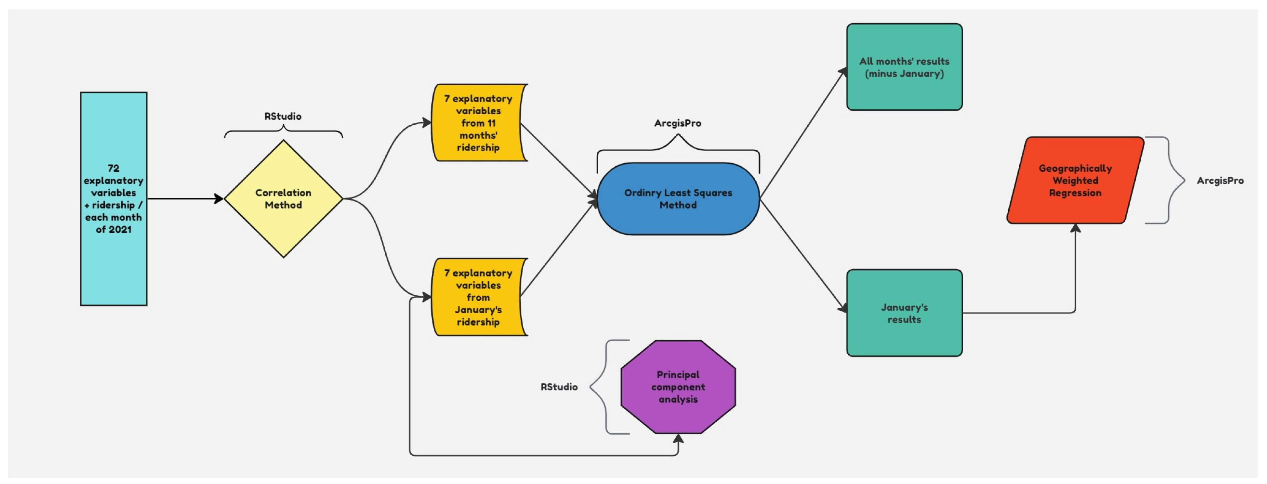
To ensure methodological coherence, the study follows an integrated analytical framework, as shown in
Figure 3, that links correlation-based variable screening, OLS regression, GWR local-coefficient diagnostics, and PCA in a sequential workflow. Correlation analysis supports the preliminary reduction in explanatory variables; OLS provides the global baseline; GWR visualizes local spatial variation in the ridership-socioeconomic relationship; and PCA reduces dimensionality to improve model stability and interpretability while preserving the most informative variance.
3. Results
A key prerequisite for applying the Ordinary Least Squares (OLS) method is ensuring sufficient degrees of freedom. In this study, the initial model included 72 explanatory variables across 66 observations (metro station catchments), resulting in negative degrees of freedom:
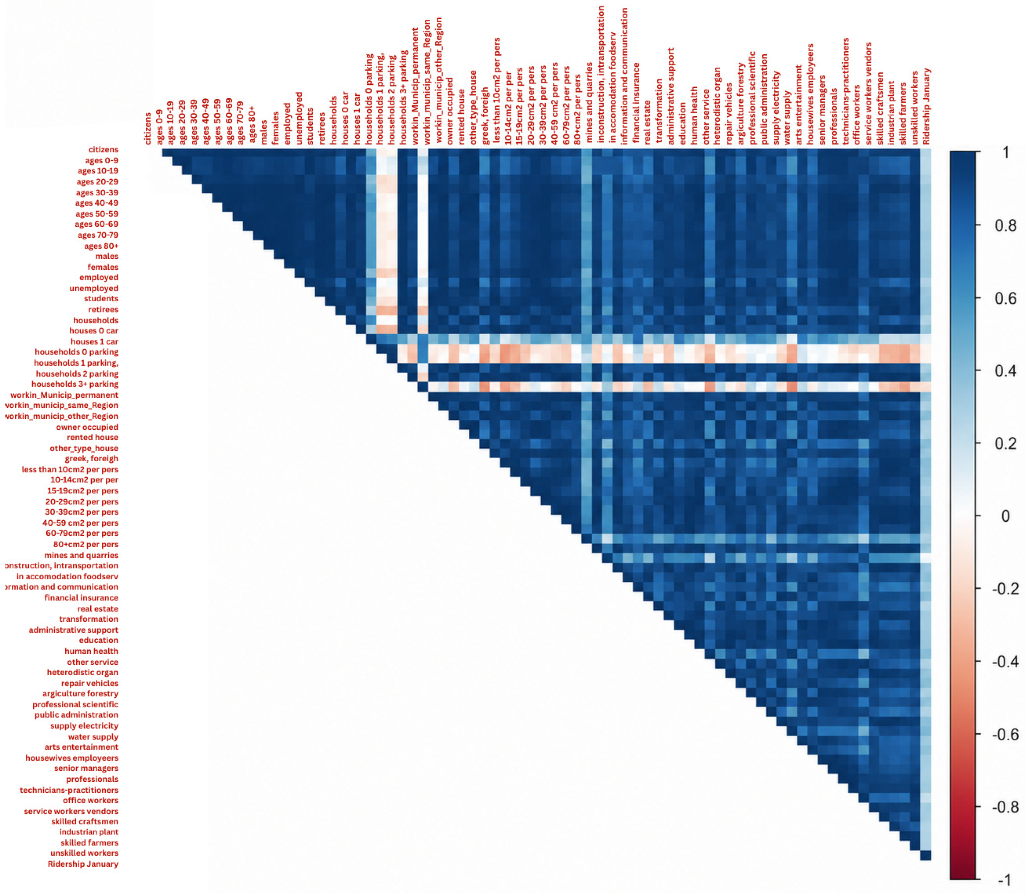
Formula (1) expresses the degrees of freedom of the OLS regression model, defined as the number of observations (N) minus the number of explanatory variables (k) and the intercept term. A negative value indicates model overparameterization, meaning that the number of parameters to be estimated exceeds the available independent information, rendering the initial model unsolvable due to insufficient independent information to estimate all coefficients. To address this, a variable reduction process was carried out using correlation analysis. RStudio was employed for its reproducibility and efficiency, as the correlation procedure had to be applied across twelve monthly ridership datasets using a consistent set of 72 socioeconomic indicators exported from QGIS. Correlation matrices, heatmaps, and filtered Excel outputs were generated to identify and exclude variables exhibiting high multicollinearity or low relevance.
For January—the reference month used in further modeling—the reduced variable set comprised: (i) number of households with one and three parking spaces, (ii) residents working in another municipality within the same regional unit, (iii) residents employed in mining and quarrying, (iv) residents working in financial and insurance activities, (v) residents employed in heteronomous organizations (e.g., diplomats, military personnel), and (vi) operators of industrial plants and machinery.
Figure 4 shows a correlation heatmap of all 72 explanatory variables and the dependent variable (Ridership for January) in RStudio.
Following the correlation analysis, a reduced set of explanatory variables was produced for each of the twelve months, resulting in twelve separate datasets. The variable set remained consistent across months, with one exception: in months other than January, the variable “operators of industrial plants and machinery” was replaced by “residents working in transport and storage.”
Using these filtered datasets, Ordinary Least Squares (OLS) regression models were implemented in ArcGIS Pro for each month of 2021. Ridership served as the dependent variable in all cases. The procedure generated twelve output reports for each month, each containing relevant statistical diagnostics, coefficient estimates, and visualizations of model performance. To identify the most statistically robust model, the monthly OLS results were systematically compared based on key indicators. Particular emphasis was placed on the Adjusted R-squared and Multiple R-squared values, as shown in
Table 1, which reflect the model’s explanatory power while accounting for the number of variables.
The comparison enabled the selection of the most suitable month—January—for further spatial analysis using Geographically Weighted Regression (GWR). March produced the highest Multiple R-squared, while January yielded the strongest balance between explanatory power, parsimony, and diagnostic stability among the monthly OLS models. Although the adjusted R-squared values were generally low, indicating limited predictive power, January was retained for detailed spatial analysis because it provided the most suitable reference month for examining regular commuting-period ridership patterns. The monthly R-squared values are therefore used to compare the global OLS models across months, while the subsequent comparison between OLS and GWR is based on AICc, as recommended for comparing models with different complexity.
For January, the global OLS model indicates modest network-wide associations between ridership and the selected socioeconomic variables. The coefficient signs suggest that parking availability, commuting geography, and selected employment categories are relevant to the interpretation of ridership differences, but the limited explanatory power and the absence of consistently strong coefficient significance mean that these effects should be interpreted as exploratory associations rather than as causal relationships. A summary of the January OLS results is shown in
Table 2.
The GWR analysis was reoriented from residual mapping to local coefficient interpretation. The AICc comparison indicates that the global OLS model has a lower AICc (1852.65) compared with the GWR model (1860.14). Therefore, GWR is not presented as a statistically superior predictive model. Instead, it is used as an exploratory spatial diagnostic to visualize how the direction and magnitude of selected socioeconomic associations vary across the network.
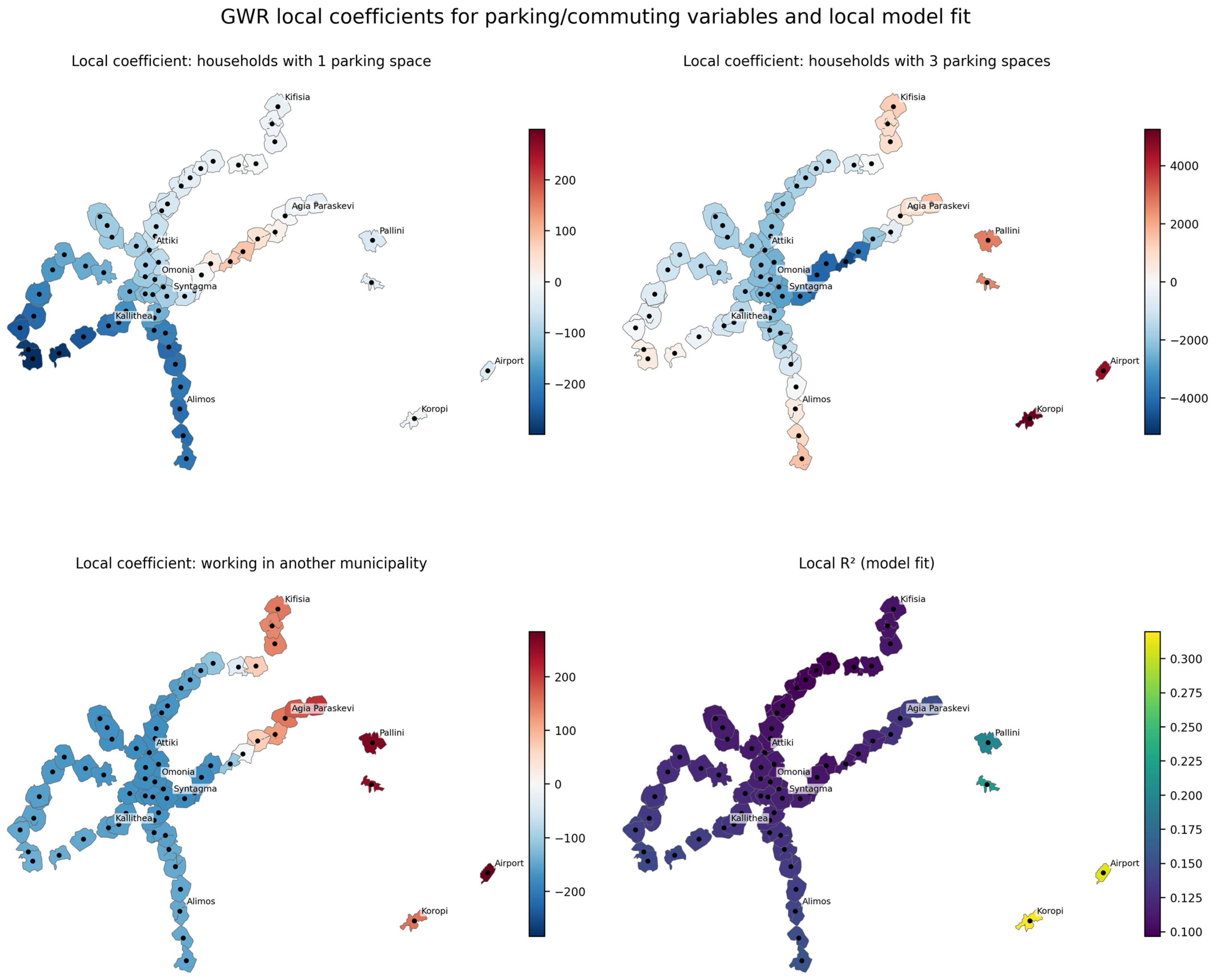
Figure 5 maps the local coefficients for the parking and commuting-related variables. The coefficient for households with one parking space is mostly negative, whereas the coefficient for households with three parking spaces varies more strongly across space. This pattern suggests that car-availability indicators do not have a uniform relationship with ridership across the metropolitan area. The coefficient for residents working in another municipality also varies spatially, highlighting differences between central and peripheral station contexts. The local R
2 panel shows that the explanatory power of the local model remains modest overall, reinforcing the exploratory interpretation of the GWR outputs.
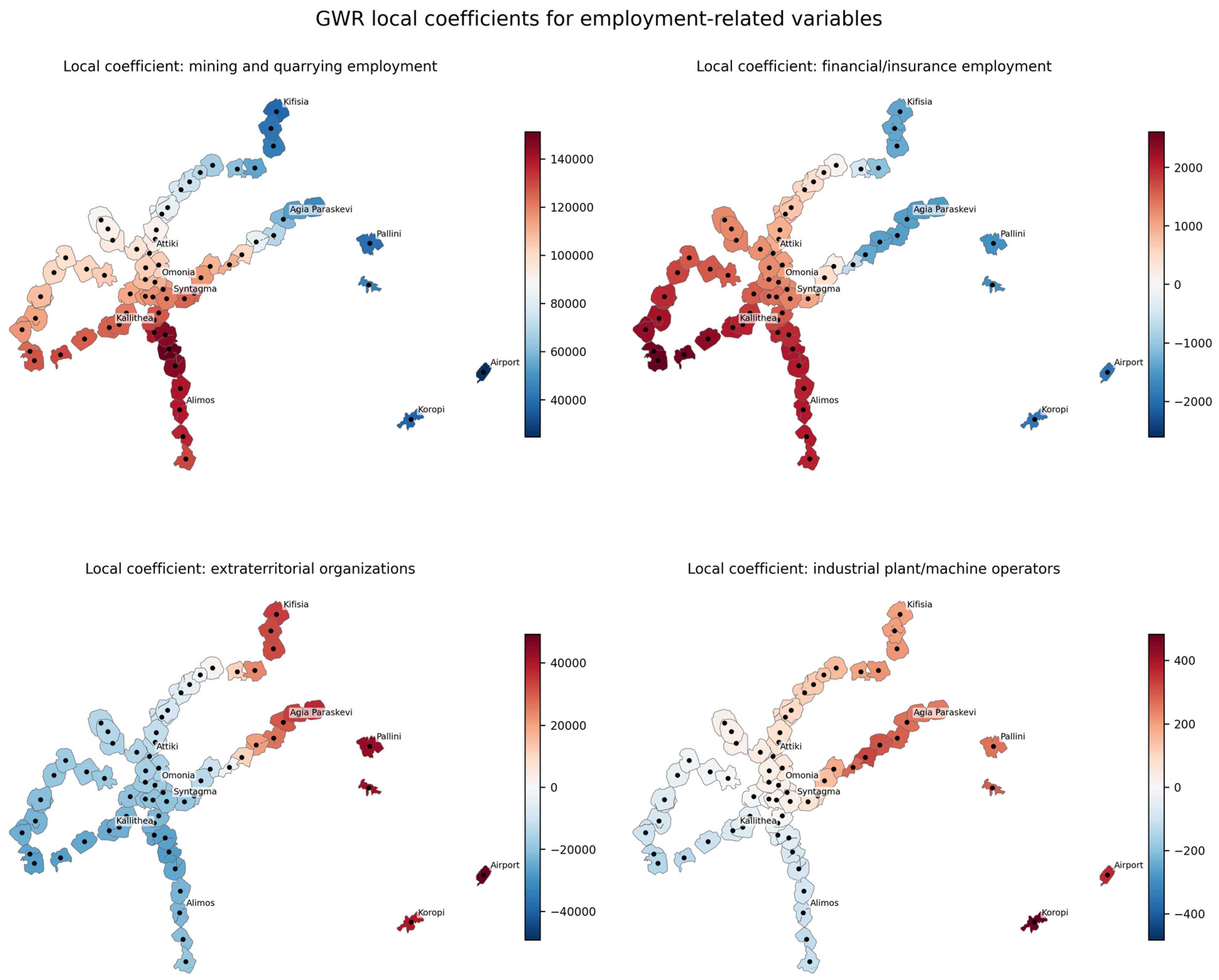
Figure 6 presents the local coefficients for the employment-related variables. Employment in mining and quarrying and financial/insurance activities generally shows spatially varying positive coefficients, while the coefficients for extraterritorial organizations and industrial plant/machine operators include both negative and positive local values. These maps provide a more direct answer to where each variable is associated more strongly or weakly with ridership than the previous residual maps. They also show that local coefficient variation exists, but it should be interpreted cautiously because the global OLS model remains preferred by AICc.
Principal Component Analysis (PCA) was conducted in RStudio using the explanatory variables retained from the January correlation analysis. PCA transforms the original variables into uncorrelated components—linear combinations designed to capture the maximum variance in the dataset while minimizing redundancy [
53].
Subsequent OLS models were tested in ArcGIS Pro using varying numbers of components. The best statistical performance was achieved using only the first two principal components, which retained most of the original information and improved model robustness, with their results shown in
Table 3 (asterisk denotes statistical significance—
p < 0.05).
The application of Principal Component Analysis (PCA) led to significant improvements in model diagnostics compared to the initial OLS results. Most notably, the Variance Inflation Factor (VIF) values, which previously ranged between 3 and 35, indicating severe multicollinearity, were substantially reduced. Following PCA, VIF values were consistently close to 1, confirming the effective elimination of multicollinearity among explanatory variables and strengthening the model’s internal consistency.
This dimensionality reduction also improved model parsimony by replacing correlated observed indicators with orthogonal components. The PCA-based specification is therefore interpreted as a stability and dimensionality-reduction check rather than as evidence of a strongly predictive model. These diagnostics support the use of PCA as a means of simplifying interrelated socioeconomic data while preserving informative variation for subsequent interpretation.
Taken together, the monthly OLS models indicate that the association between ridership and station-area socioeconomic characteristics is not temporally constant. Higher adjusted R-squared values in January and March suggest that local socioeconomic structure is more closely related to metro demand during months dominated by regular commuting, whereas the weaker fit observed in the summer months reflects seasonal changes in activity patterns and a less stable relationship between ridership and residential catchment characteristics.
For January, the OLS model provides the global, network-wide picture. At this aggregate level, the retained socioeconomic variables explain only a modest share of ridership variation. The coefficient directions suggest links with parking availability, commuting geography, and employment structure, but these global effects should be interpreted cautiously, given the limited explanatory power of the model.
The GWR coefficient maps refine this picture descriptively by showing that the strength and direction of selected associations are not spatially uniform. However, because the GWR model has a higher AICc than the global OLS model, these local coefficient patterns are treated as exploratory spatial diagnostics rather than as evidence that GWR provides a better overall model fit.
PCA further supports this interpretation by showing that a reduced set of latent socioeconomic dimensions can improve model stability even when predictive power remains modest. Overall, the results suggest that metro ridership in Athens is shaped by a combination of network centrality, local socioeconomic context, and seasonal variation, and that these influences are spatially uneven rather than uniform across the system.
4. Discussion
This study set out to examine how station-area socioeconomic characteristics relate to metro ridership in Athens, how these relationships vary spatially, and what the combined use of global and local analytical techniques contributes to interpretation.
The findings show that ridership is associated most clearly with employment structure, commuting geography, and car-related household characteristics, although these associations remain modest at the network-wide level. This limited explanatory power indicates that socioeconomic conditions represent only one part of the ridership mechanism and should be interpreted alongside omitted operational factors such as service frequency, connectivity, fares, travel times, and interchange intensity.
Regarding spatial variation, the results suggest a clear distinction between central interchange stations and peripheral or suburban stations. In central locations such as Syntagma, Omonia, and Attiki, ridership is high but only partially captured by local socioeconomic variables because these stations concentrate network effects, transfers, and metropolitan-scale destinations.
In outer station areas, by contrast, local accessible catchment characteristics appear to show stronger exploratory associations with ridership, implying that access conditions, residential composition, and dependence on private cars may play a more direct role in shaping demand. These findings should be interpreted as exploratory station-catchment associations, given that the accessibility catchments are not mutually exclusive. In this sense, the study interprets equity descriptively as the uneven ability of different areas and socioeconomic groups to benefit from metro accessibility, rather than as a direct normative measure of fairness.
These findings have several planning implications. For central stations, priorities should include interchange efficiency, crowd management, pedestrian circulation, and multimodal integration, since demand there is driven less by local catchment composition than by the station’s role within the wider network.
For peripheral and suburban stations, interventions should focus on first/last-mile accessibility, feeder public transport, walkability, and land-use coordination, because local socioeconomic structure appears to matter more directly. The negative association with variables linked to geographically dispersed work patterns and car-oriented households also suggests that outer Attica station areas may face structural barriers to regular metro use; therefore, low ridership in these areas should not automatically be interpreted as low need, but potentially as evidence of constrained access or car dependency.
Methodologically, the study shows the value of a combined workflow in which OLS provides a global baseline, GWR visualizes local coefficient variation, and PCA stabilizes interpretation under a high-dimensional set of correlated socioeconomic indicators. The AICc comparison indicates that the global OLS model remains preferable in terms of model parsimony, while the GWR maps remain useful as exploratory visual diagnostics of spatially varying associations.
The framework is thus best understood as an exploratory analytical workflow rather than as a strongly predictive modeling framework. The relatively low adjusted R-squared values, the higher AICc of GWR compared with OLS, and the aggregate nature of the available ridership data all indicate that the results should be read with appropriate caution.
Therefore, several limitations of the study should be acknowledged. First, the explanatory power of the global models remains modest, which means that the findings should be interpreted primarily as exploratory spatial associations rather than as strong predictive relationships. Second, the analysis relies on aggregate monthly station-level ridership data that do not distinguish boarding from alighting movements, trip purpose, or fare-user categories, thereby limiting finer behavioral interpretation. Third, the socioeconomic variables represent census-based counts within station catchments and therefore act as proxies for local context, without directly capturing land-use intensity, destination attractiveness, service frequency, network connectivity, fares, travel times, or interchange activity. Fourth, the 10 min walking isochrones used in this study are not mutually exclusive and may overlap in parts of the Athens Metro network. Consequently, the same residential or socioeconomic area may contribute to more than one station catchment, potentially introducing double-counting in the explanatory variables. This does not affect the interpretation of the catchments as potential accessibility areas, but it limits the interpretation of the regression coefficients as strictly independent station-area effects. Future work could also test the robustness of the findings by intersecting walking isochrones with Thiessen/Voronoi polygons, thereby assigning each area to only the nearest station once, where this may be more suitable considering varying urban environments, before recalculating socioeconomic indicators and re-estimating the models. Fifth, although monthly OLS models were estimated for all months of 2021, the local spatial analysis focuses on January as the most statistically robust month; therefore, the GWR coefficient maps should not be generalized uncritically to all seasonal conditions. Finally, the study does not include formal residual spatial autocorrelation diagnostics or alternative spatial econometric specifications, such as spatial lag/error models or MGWR. These limitations do not invalidate the spatial patterns identified here, but they do mean that the findings should be interpreted as indicative associations rather than causal relationships.
Overall, the analysis highlights that metro ridership disparities in Athens cannot be explained by a single metropolitan-wide relationship. Instead, demand reflects a layered interaction between network role, local socioeconomic composition, and spatial context. For practitioners, this implies that a uniform policy approach is unlikely to be effective across the entire network. For researchers, it suggests that future work should combine richer operational variables, formal spatial dependence diagnostics, and multimodal data to further refine the interpretation of accessibility-related inequalities.