Article

Comparative Assessment of Quantitative Landslide Susceptibility Mapping Using Feature Selection Techniques

by
Buddhi Raj Joshi
1,
Netra Prakash Bhandary
2,*,
Indra Prasad Acharya
3 and
Niraj K.C.
4
1
School of Engineering, Faculty of Science and Technology, Pokhara University, Kaski 33700, Nepal
2
Faculty of Collaborative Regional Innovation, Ehime University, Matsuyama 790-8577, Japan
3
Department of Civil Engineering, Pulchowk Campus, Institute of Engineering, Tribhuvan University, Lalitpur 44700, Nepal
4
Department of Geomatics Engineering, Pashchimanchal Campus, Institute of Engineering, Tribhuvan University, Kaski 33700, Nepal
*
Author to whom correspondence should be addressed.
ISPRS Int. J. Geo-Inf. 2026, 15(1), 20; https://doi.org/10.3390/ijgi15010020 (registering DOI)
Submission received: 30 October 2025 / Revised: 23 December 2025 / Accepted: 28 December 2025 / Published: 1 January 2026

Abstract

Landslide susceptibility mapping is crucial for landslide risk management in mountainous areas like Nepal. However, the performance of a landslide susceptibility model is often compromised by multicollinearity among landslide causative factors. While feature selection techniques are recognized as essential preprocessing steps, most studies lack systematic comparisons of how different selection methods affect traditional models under identical conditions. This study addresses this gap by evaluating Weighted Overlay (WO), Multiple Linear Regression (MLR), and Logistic Regression (LR) using Correlation Analysis, Variance Inflation Factor (VIF), and Information Gain (IG) feature selection techniques. It is found that LR with Correlation Analysis results in 69.30% accuracy and 75.48% Area Under the Receiver Operating Characteristic Curve (AUC-ROC) while maintaining balanced precision (64.47%) and recall (85.96%). The WO model yields outstanding landslide recognition (90.18% recall) with VIF analysis despite a lower precision value (56.74%). MLR with IG analysis achieves reliable performance (62.11% accuracy, 64.76% AUC-ROC) for regional assessments. The study offers practical guidelines for method selection based on assessment goals, emphasizing the trade-off between statistical optimization and physical interpretability in susceptibility mapping.

1. Introduction

Landslides are among the most damaging geological events worldwide. They cause significant loss of human life and damage to physical infrastructure as well as the ecology of the regions with steep terrain, unstable soil, and heavy precipitation. In hilly and mountainous areas, landslide initiation is rarely attributable to a single factor. Still, it is instead the product of a complex interplay between predisposing geological structures, steep topographical gradients, and preparatory environmental agents such as intense rainfall and anthropogenic activities [1,2,3]. Although the multi-factor nature of landslides is well-recognized, it presents a significant analytical challenge. The causative factors are often statistically interdependent (multicollinear), which can compromise the performance and interpretability of quantitative landslide susceptibility models if not properly addressed [3,4,5].
Landslide Susceptibility Mapping (LSM) is a vital tool for disaster risk reduction, focusing specifically on the spatial likelihood of landslide occurrence based on terrain conditions. This concept differs from landslide risk, which incorporates the exposure and vulnerability of elements such as population and infrastructure [4,5]. The field has evolved from interpretable traditional models, including WO, MLR, and LR, to advanced machine learning techniques. While these newer approaches often offer greater predictive accuracy, traditional models remain highly relevant for operational use due to their interpretability and ease of implementation [6,7]. These models predict susceptibility by analyzing the influence of various causative factors, such as elevation, slope, rainfall, and geology [6,7,8]. However, their effectiveness is frequently compromised by an oversimplification of complex, non-linear relationships [3,9] and, more critically, by multicollinearity, the strong statistical interrelations between factors like elevation, slope, and aspect [10]. This multicollinearity increases model variability, decreases interpretability, and can result in inaccurate susceptibility maps.
In parallel, the LSM field has experienced significant advancements with the development of probabilistic physical and hybrid modeling frameworks. These approaches integrate geotechnical principles, such as limit equilibrium or infinite slope stability models, with statistical and spatial data to quantify slope stability under varying hydrological and seismic conditions [11,12,13,14]. Physics-informed models often incorporate uncertainty propagation and can provide a more mechanistically transparent assessment of landslide susceptibility, particularly at site-specific or process-dominant scales. At regional scales, hybrid frameworks that combine physical stability concepts with statistical or machine learning models have emerged to balance physical consistency with data-driven adaptability [10,11,15]. While these sophisticated frameworks offer high interpretability and strong physical grounding, they typically require detailed geotechnical and hydro-mechanical input data that are often unavailable across large, data-scarce mountainous regions. Our study, in contrast, focuses on widely applicable, data-efficient traditional models (WO, MLR, LR) and rigorously evaluates how standard feature selection techniques can optimize their performance under common data constraints. In doing so, we provide a practical, scalable pathway to improve susceptibility mapping in regions where advanced physical modeling is not yet feasible, while also highlighting the trade-offs between statistical optimization and physical representativeness that inform future hybrid approaches [16].
The realm of LSM has progressed profoundly because of the machine learning (ML) and Deep Learning (DL) models, which are proficient at handling complex, non-linear relationships and have significantly achieved high predictive performance [17]. Despite the visible advancement in the field, the commonly used traditional models like WO, MLR, and LR remain highly relevant for operational use, primarily due to their advancing these highly established models. This study aims to advance these highly established models by turning to feature selection as a critical preprocessing step to address their limitations. Three recognized techniques are adopted: Correlation Analysis, Variance Inflation Factor (VIF), and Information Gain (IG). Each method acts as a unique function: Correlation Analysis ascertains linear relationships between variable pairs, VIF directly helps in quantifying the degree of multicollinearity, and IG ranks features by their predictive power through entropy reduction [18]. Whereas previous studies in general employ only one or two such methods in different contexts [19,20,21], this study in particular presents a systematic and quantitative comparison of these highly accepted and widely used models (WO, MLR, LR), each deployed alongside these three feature selection techniques in a systematic way. This direct comparison allows for a unique analysis of their interactions, which is a comprehensive methodology seldom explored in the existing literature. However, the systematic integration and comparison of these distinct techniques with traditional LSM practices are insufficiently addressed in this domain [22,23].
Beyond empirical performance comparisons, a critical scientific question remains unexamined: do different feature selection techniques operate consistently under common geomorphic and hydrological constraints, or do they introduce systematic physical bias into landslide susceptibility models? For instance, while VIF eliminates multicollinear variables to ensure statistical independence, it may inadvertently remove geomorphologically relevant factors that co-vary due to shared physical processes (e.g., slope and curvature) [24]. Conversely, IG prioritizes predictive power but may retain correlated variables that obscure interpretability and inflate model instability [25]. Correlation Analysis, while intuitive, may overlook nonlinear dependencies essential in hydrological and geotechnical systems [26].
Hence, this study not only fulfills a methodological gap by conducting a straightforward, quantitative comparison of MLR, WO, and LR models each integrated with three feature selection techniques but also explicitly tests the following hypothesis: Feature selection methods influence not only model performance but also the physical consistency and interpretability of landslide susceptibility maps, with each technique introducing distinct biases in how geomorphic, hydrological, and anthropogenic factors are represented. Furthermore, by detailing a transparent factor selection rationale, this study aims to provide a transferable framework that can enhance methodological consistency in LSM across diverse geological settings. Through a detailed evaluation of results with metrics like AUC, recall, precision, and spatial pattern analysis, this study examines how feature selection harmonizes or distorts the representation of landslide causality in traditional LSM frameworks. The findings aim to provide not only practical insights for improving landslide prediction but also a mechanism-informed rationale for method selection, advancing LSM toward more reliable and physically interpretable mapping in diverse geological settings.

2. Material and Method

2.1. Study Area
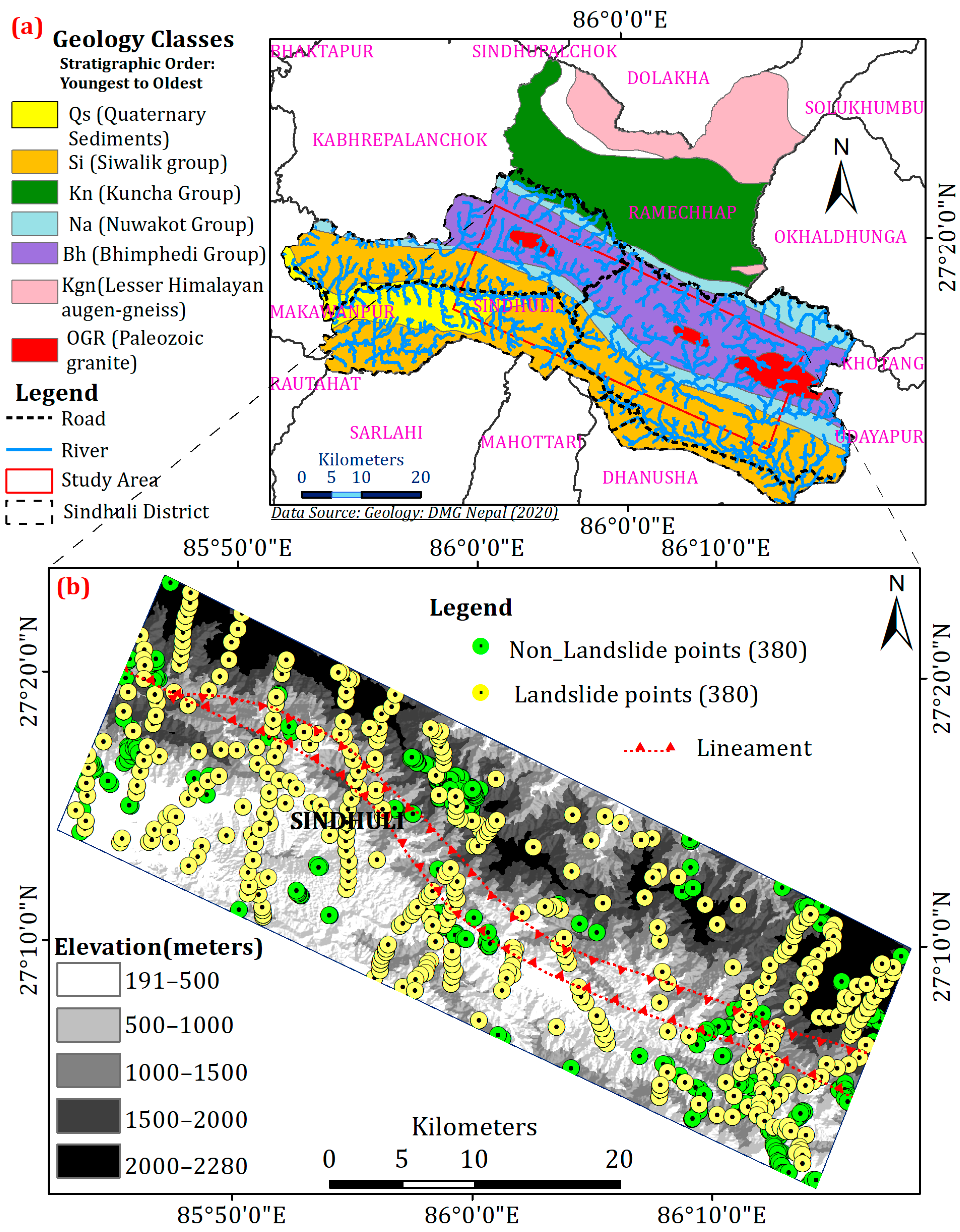
This study was conducted on a landslide-prone area in the mid-Himalayan mountains, which lies in the northern Sindhuli District of Nepal, with a geographical location of 27.016° S–27.394° N and 85.709° W–86.304° E (Figure 1). The area encompasses a complex geological setting, featuring formations including the Quaternary alluvium (unconsolidated sediments), Siwalik Group sandstones, Kuncha Group metamorphic rocks, mixed clastic rocks of the Nuwakot Group, metamorphic quartzites of the Bhimphedi Group, and resistant Ordovician granites [27,28]. The varied lithology and structural features of these units, particularly the weak, unconsolidated sediments and sheared metamorphic rocks, are primary contributors to slope instability in the region [27,28].
Sindhuli District has an elevation range of 300 to 3000 m. This range creates four distinct ecological zones. The tropical lowlands from 300 m to 1000 m support rice and maize cultivation, the subtropical mid-lands from 1000 m to 2000 m contain mixed forests, the temperate highlands from 2000 m to 3000 m feature alpine vegetation, and areas above 3000 m have freezing pastures [29]. This region receives an annual average rainfall of more than 1500 mm, which causes highly saturated soil conditions, leading to frequent soil erosion and the mass wasting process. Moreover, road development and deforestation have aggravated the region’s susceptibility to landslides. So, the unstable soil structure, wider elevation range, excessive rainfall, and anthropogenic effects all make this area an optimal site for landslide susceptibility modelling as our research questions demand [29].
Figure 1. Location map of the study area in Sindhuli District of Nepal: (a) geological outline map showing lithological units in stratigraphic order (youngest to oldest) including Qs, Si, Kn, Na, Bh, Kgn, and OGR, overlaid by major roads, rivers, and administrative boundaries for spatial reference and (b) elevation map including the landslide and non-landslide point locations that were used for analysis in this study. (Note: The geological outline map is based on 1:50,000 geological map data availed by the Department of Mines and Geology (DMG) of Nepal, 2020 edition [30]).
Ijgi 15 00020 g001

2.2. Data and Software Employed

Multiple datasets were used in this study for the landslide susceptibility analysis, which can be categorized into four groups: landslide inventory data, rainfall data, geology and soil data, and remote sensing data. All spatial processing was performed in ArcMap 10.7, while statistical analysis and modeling were performed in Python 3. A 30-m resolution ASTER Digital Elevation Model (DEM) served as the base topographic layer. To maintain temporal consistency, all datasets were aligned with the landslide inventory period corresponding to 2015–2020.
Landslide inventory was compiled from the Google Earth imagery and field surveys (2015–2020). Topographic parameters (i.e., elevation, slope, aspect) and secondary geomorphological indices (i.e., Topographic Wetness Index–TWI and Stream Power Index–SPI) were derived from the DEM. The DEM also enabled the extraction of the hydrographic network for assessing fluvial undercutting. Specifically, the river network was derived using the D8 flow direction algorithm in ArcGIS 10.8, followed by the calculation of flow accumulation. A threshold of 1000 contributing cells (equivalent to a drainage area of approximately 0.9 km2) was applied to define perennial streams, ensuring that only significant channels influencing slope stability were retained for the distance to river factor.
Likewise, Sentinel-2A imagery from the 2019–2020 dry season was used to compute vegetation and built-up indices (i.e., MNDVI, ARVI, NDBI), which were derived from Equations (1)–(3) [30,31,32].
M N D V I = N I R R e d N I R + R e d
A R V I = N I R ( 2   Red   B l u e ) N I R + ( 2   Red   B l u e )
N D B I = N I R R e d N I R + R e d
where NIR, Red, and Blue refer to the reflectance values of the respective Sentinel-2 bands. Cloud-free composites were generated using the median value of all available scenes during the dry season to minimize atmospheric and seasonal variabilities.
CHIRPS rainfall data (version 2.0, 5 km resolution, 2015–2020) were aggregated to mean annual precipitation [33]. Soil data were obtained from the SOTER database of Nepal (scale 1:1,000,000) [34], and geological data including the major geological structures (e.g., faults and thrusts) were obtained out of 1:50,000 scale geological map, 2020 edition published by the Department of Mines and Geology (DMG), Nepal [35]. Their surface traces were then verified and refined using the DEM-derived hill shade and slope models to ensure accurate geomorphic representation.
Moreover, the road network in the study area was extracted from OpenStreetMap (OSM, 2020 download) [36]. Higher-resolution datasets (e.g., 10 m Sentinel-2A indices, 5 km CHIRPS) were resampled to a 30-m DEM grid using bilinear interpolation to ensure spatial consistency. Sample selection included 380 landslide points obtained as polygon centroids and 380 non-landslide points generated via stratified random sampling in stable areas (slope < 5°, outside landslide zones). A 100-m buffer was maintained between landslide and non-landslide points to reduce spatial autocorrelation. The combined dataset of landslide and non-landslide points (total: 760 points) was randomly split into 70% training and 30% testing datasets for the model development and evaluation purpose, respectively.

2.3. Landslide Susceptibility Mapping (LSM)

This study investigates the impact of common feature selection strategies on traditional landslide assessment models. Specifically, Correlation Analysis, Variance Inflation Factor (VIF), and Information Gain (IG) methods are systematically applied to Weighted Overlay (WO), Multiple Linear Regression (MLR), and Logistic Regression (LR) frameworks to identify optimal model-feature combinations. Each feature selection method outlines unique benefits: Correlation Analysis filters variables through pairwise linear relationships. VIF prioritizes statistical independence by eliminating multicollinear factors. IG selects features based on their predictive contribution to landslide classification. The analysis reveals specific performance patterns across different evaluation metrics by providing tailored recommendations for selecting feature selection methods in LSM, based on specific application needs in general.
This study follows a structured four-stage methodology, as depicted in Figure 2. The process begins with data preprocessing to clean and prepare the dataset. Subsequently, feature selection is performed to identify the most significant predictors. The third stage involves model selection and training, where various algorithms are evaluated. Finally, the methodology concludes with a comprehensive model evaluation to quantify performance. The ensuing sub-sections elaborate on each stage, detailing the specific techniques employed for data preparation, the criteria for feature selection, the range of models investigated, and the metrics used for evaluation.

2.3.1. Landslide Causative Factor Classification and Normalization

As presented in Table 1, we utilized 15 causative factors for LSM in this study. The initial set of causative factors was decided through a comprehensive review of LSM literature in comparable Himalayan terrain [4,10,17,21]. The final selection, however, was guided by a structured, three-tiered rationale designed to ensure both scientific validity and methodological transparency. At first, the factors were retained based on their physical relevance, requiring a clear mechanistic link to landslide initiation, such as slope angle for shear stress and the TWI for soil saturation, as established in foundational geotechnical literature [19,37]. Next, we prioritized factors with strong regional diagnostic value for the Nepal Himalaya, including proximity to roads and rivers as proxies for anthropogenic and fluvial destabilization [21,29], as well as specific lithological units like the Siwalik Group, which are widely recognized for their instability [27,28]. Then, to promote operational transferability, we emphasized this selection framework over a static factor list. The framework centered on assessing mechanism, diagnostic value, and data availability, provides a structured, repeatable rationale. It can be directly adapted to other regions by substituting locally relevant diagnostic variables (e.g., distance to irrigation canals in agricultural settings or specific weak volcanic units) while maintaining core geomorphic and geotechnical principles.
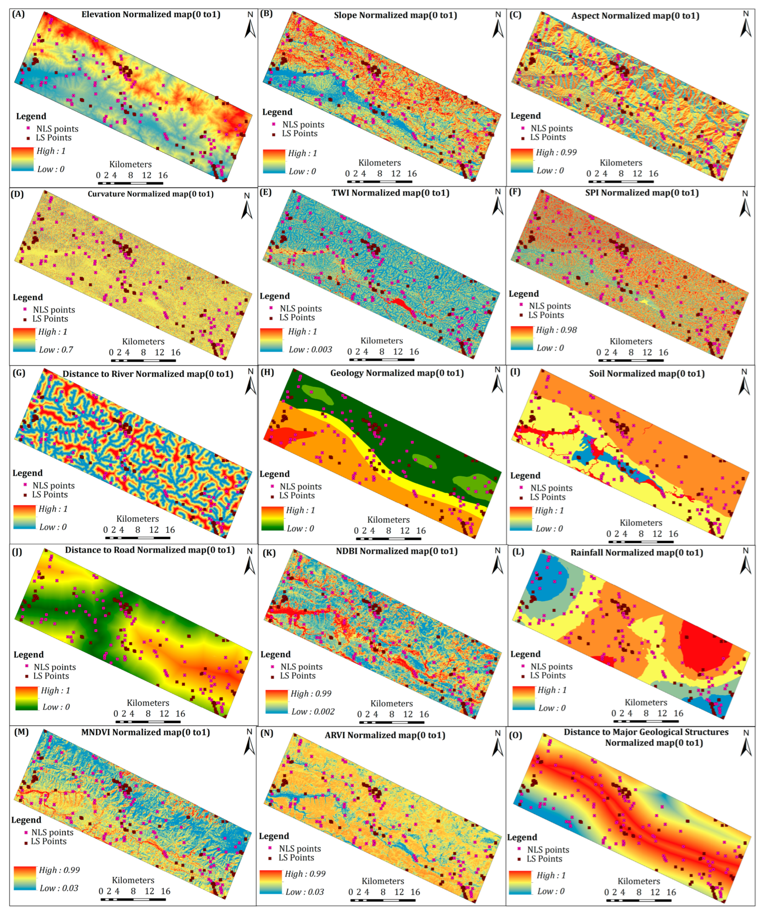
Each continuous factor was classified into five categories using the natural breaks (Jenks) method, with thresholds adjusted according to established geomorphological principles (e.g., slope stability thresholds, soil saturation limits). All values were normalized to a 0–1 scale using min–max scaling. The normalization process creates consistent data ranges. It preserves original data relationships. The method uses the actual dataset’s minimum and maximum values. This approach supports scientific validity without forcing extreme values. The normalized landslide causative factor maps with landslide and non-landslide points are presented in Figure 3 while the factor and class relevancy descriptions are made as follows.
Elevation influences landslide susceptibility through gravitational stress, so stable elevation range below 500 m was considered to have minimal landslide risk (0.0), while comparatively unstable heights from 500 m to 2000 m were assigned progressively increasing risk values from 0.25 to 1.0 (Figure 3A). Slope angle is a critical destabilizing factor [37], so it was categorized as gentle slopes below 10 degrees with low risk (0.0), 10–20 degrees with 0.25, 20–30 degrees with 0.5, 30–40 degrees with 0.75, and slopes steeper than 40 degrees with the highest risk (1.0) (Figure 3B). Likewise, the Aspect, which influences weathering through solar exposure and moisture retention, was rated with north-facing slopes as the most stable (0.0) and south-facing slopes as the most vulnerable (1.0) (Figure 3C). Moreover, as Curvature is a measure of slope tension and susceptibility to cracks, it was classified with flat slopes rated as 0.0 and highly convex slopes as 1.0 (Figure 3D).
The water-related parameters, such as TWI, SPI, and distance to rivers, heavily influence the landslide susceptibility of an area. TWI indicates the saturation zones [38], so the dry areas with TWI < 5 were classified as 0.0, TWI 5–7 as 0.25, TWI 7–9 as 0.5, TWI 9–11 as 0.75, and TWI > 11 with lasting saturation and highest risk as 1.0 (Figure 3E). Likewise, SPI measures the erosive potential of a stream [21], which in this study has been categorized as: SPI < 3 as 0.0, SPI 3–6 as 0.25, SPI 6–9 as 0.5, SPI 9–12 as 0.75, and SPI > 12 was classified 1.0 with maximum risk of erosion (Figure 3F). Additionally, distance to rivers also affects landslide susceptibility. The highest susceptibility with 1.0 was considered for the areas within 200 m of the river proximity, and it decreased with greater distances, reaching 0.0 beyond 1600 m (Figure 3G).
With regard to the geology, a landslide risk-based rating system for the geological units was applied: well-consolidated sedimentary rocks were considered to have low ratings of 1 to 2, loose deposits like Quaternary Alluvium (Qs) and Siwalik sediments (Si) were considered to have high ratings of 4 to 5, and intermediate formations (Na) were considered to have medium rankings. The final geological framework ranged from 0.0 for resistant rocks to 1.0 for weak, unconsolidated deposits, as shown in Figure 3H.
Likewise, soil categories were prioritized on the basis of stability and erosion tendency: Haplic Phaeozems (PHh) was assigned a score of 1 for its high resistance to erosion, Cambisols (CMe) was given 2 for moderate stability, Dystric Regosols (RGd) was given 3 for its weak development, and Gleyic Cambisols (CMg) was given 4 for its high waterlogging capacity and instability. The soil classification system ranged from stable sandy soils (0.0) to unstable pure clay (1.0), as shown in Figure 3I.
Moreover, a spatial analysis revealed that there is a strong cluster of landslides near roads and rivers, as presented in Table 2. The data indicate that 1668 landslides (78%) occurred within 500 m from the roads and 1604 landslides (75%) occurred within 500 m from the rivers. However, it is emphasized that these road and river proximity factors are not the direct triggers of landslides.
Roads and rivers were framed as spatial proxies for environmental disturbance. Roads indicate areas of anthropogenic slope modification while rivers and natural drains indicate zones of fluvial undercutting and soil saturation. These factors identify broader zones of landscape destabilization, which supports the goal of regional susceptibility modeling and justifies the inclusion of distance to roads and distance to rivers as landslide causative factors.
We consider human impact in terms of two causative factors: distance to roads and normalized difference built-up index (NDBI) [38]. The distance to roads ranges from less than 200 m to more than 1600 m (Figure 3J) while the NDBI includes land cover types, ranging from natural landscapes (below −0.2) to dense urban areas (above 0.5).
Furthermore, the environmental factors include annual rainfall intensity and vegetation indices. The rainfall ranges from less than 500 mm to more than 2000 mm (Figure 3L) while vegetation indices are represented by MNDVI and ARVI. As a measurement of vegetation cover density, MNDVI ranged from 0.6 for full density to zero for bare soil (Figure 3M) while ARVI, which performs better in hazy atmospheric conditions [39,40] ranged from –0.07 to 0.92.
One of the important landslide causative factors is geological structure, which includes proximity to mapped faults and thrusts, representing zones of structural weakness, groundwater movement, and reduced shear strength. Distance to major geological structures ranged from less than 200 m to more than 1600 m (Figure 3O).
All landslide causative factors were processed using proper classification methods and the normalization technique was employed to enable direct comparison of all causative factors. This systematic approach provides reliable inputs for the three susceptibility models in this study: WO, MLR, and LR.

2.3.2. Feature Selection Techniques

After normalizing and standardizing the 15 landslide causative factors, correlation analysis, VIF, and IG were used as feature selection techniques, which helped combine the selected causative factors using 70% of the training data. This careful process maximized model accuracy while decreasing multicollinearity, ultimately leading to selecting important factors for application in landslide susceptibility modeling using WO, MLR, and LR to create robust LSMs.
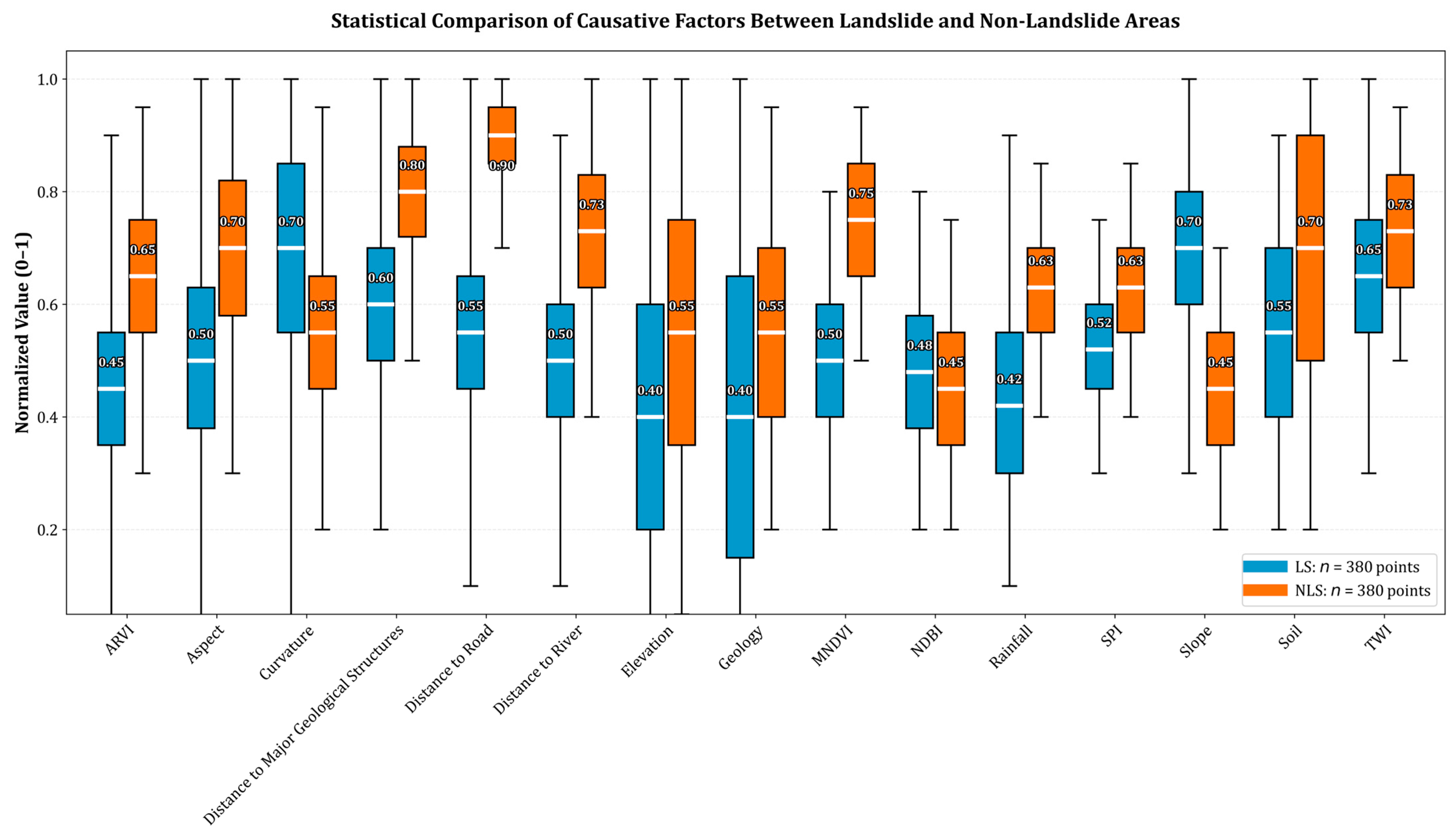
Moreover, a comparative statistical analysis was conducted to enhance the interpretive value of the causative factor maps of Figure 3 by examining how the distribution of each factor differs between landslide (LS: n = 380 points) areas and non-landslide (NLS: n = 380 points) areas. As presented as comparative boxplots in Figure 4, the results help visualize the normalized values (0–1) of each factor. Several factors exhibit pronounced distributional contrasts: for instance, NDVI, rainfall, distance to road, and distance to river display clearly separated medians and limited overlap between the LS and NLS groups, underscoring their strong potential as discriminators of landslide susceptibility. Conversely, factors such as elevation and geology show substantial overlaps, suggesting a weaker individual predictive signal in the study area. This statistical comparison not only strengthens the physical justification for factor inclusion but also provides an empirical basis for the subsequent feature selection steps. Each of these feature selection techniques is outlined as case studies in the following paragraphs.
Case 1 (Correlation Analysis): To analyze and identify relationships between landslide conditioning factors, we used both the Pearson correlation coefficient (r) and the Spearman correlation coefficient (ρ). Pearson correlation coefficient (r) measures the linear relationships between continuous variables and is determined as in Equation (4) [41].
r = i = 1 n     x i x y i y i = 1 n     x i x 2 i = 1 n     y i y 2
where x i and y i are individual sample points of the two variables, x and y are their respective means, and n is the number of data points. We used the Pearson correlation coefficient ( r ) to find and remove duplicating factors and selected those with the best physical relationships. When two factors were highly correlated (i.e., r   >   0.7 ), the variable with the stronger absolute correlation to the landslide inventory was retained, provided it also held clear physical relevance to landslide processes. If physical interpretability was similar, the factor with the higher correlation to the inventory was selected to maximize predictive association. This process ensured the removal of redundant predictors while preserving the most statistically and physically meaningful variables. The examination tested all factor permutations under rigorous statistical significance ( p < 0.01 ).
Spearman Rank & Kendall Tau (p, τ): This study evaluated nonlinear relationships using Spearman p and Kendall τ correlation tests. These tests function effectively with non-normal data distributions. The analysis methods detected monotonic variables. This detection helped select relevant causative factors [42].
Point-Biserial Correlation: This study used point-biserial correlation [43] to link the binary landslide data (stable = 0 vs. landslide = 1) with continuous causative factors. This analysis employed a correlation approach consistent with the Pearson method to assess the strength and direction of the relationship between the binary and continuous data pairs.
Case 2 (VIF Analysis): Multicollinearity, the high correlation among predictor variables, compromises model stability and interpretability, and to quantify the multicollinearity among the predictor variables, we used the VIF, which is expressed as Equation (5) [44].
V I F i = 1 1 R i 2
where Ri2 denotes the coefficient of determination in the linear regression model. The VIF for each factor was initially calculated in a linear regression model containing all 15 causative factors. An iterative elimination process was then applied: at each step, the factor with the highest VIF value exceeding 5 was removed, the VIFs for the remaining factors were recalculated, and the process was repeated until all retained factors had VIF < 5. This stepwise removal ensured that the final set of predictors was statistically independent, minimizing multicollinearity while retaining variables with direct relevance to landslide mechanisms.
Case 3 (IG Analysis): Information Gain (IG) assesses a factor’s importance for landslide prediction by measuring how much it reduces the uncertainty of landslide occurrence. Before the IG calculation, all continuous causative factors were discretized into five classes using the quantile (equal frequency) method to ensure each bin contained approximately the same number of samples. This approach mitigates the influence of extreme values and supports stable entropy estimation. Factors with higher IG values were considered more significant for landslide prediction. The importance of each landslide causative factor was then quantified using Equation (6) [45].
I G T , A = E n t r o p y T v v a l u e s A T v T E n t r o p y T v
The importance of each landslide causative factor was determined by IG analysis, which calculates entropy reduction. In this context, in Equation (6), A represents the entire set of causative factors, T denotes the binary presence or absence of landslide locations, and Tv signifies a data subset where factor A equals a specific class v. We applied standard IG calculations to every variable, ensuring robust estimation through 10-fold cross-validation. Then, we interpreted the results using a 0–1 score system, in which a score closer to 1 indicates higher predictive importance.

2.3.3. Model Selection

Three conventional modeling techniques generated landslide susceptibility maps, which include Weighted Overlay, Multiple Linear Regression, and Logistic Regression, which are separately described as follows.
Weighted Overlay (WO): In this method, each landslide causative factor is given a weightage based on how important it is for the landslides to occur, and it was determined using Equation (7) [46].
L S M = i = 1 n w i × x i
where w i and x i are the weight of causative factors and the normalized value of each landslide causative factor, respectively. The weights ( w i ) for the WO model were derived directly from the results of each feature selection technique as follows:
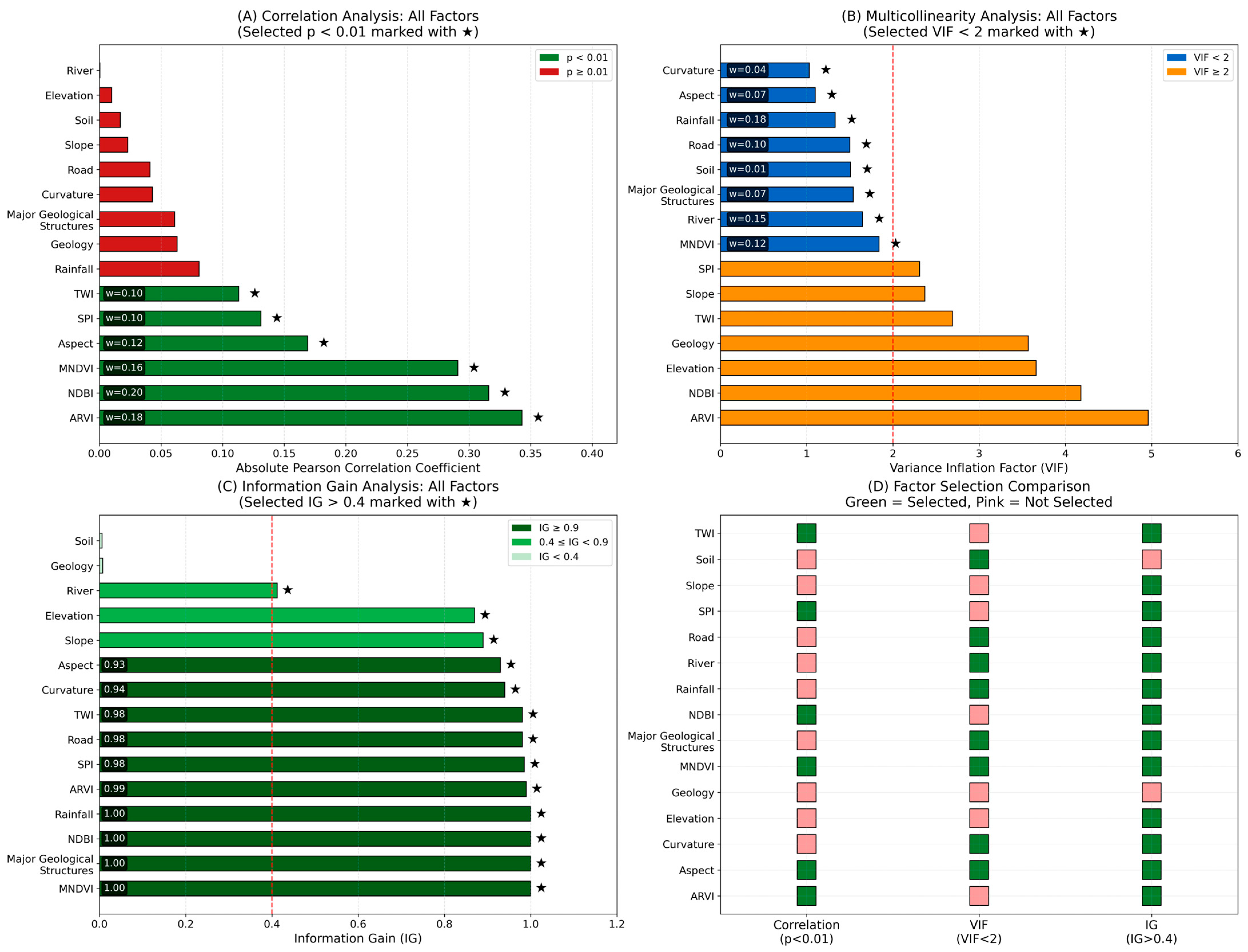
First, for the correlation analysis (Case 1), the absolute values of the Pearson correlation coefficients between each factor and landslide occurrence were summed up. Each factor’s weight was then calculated as its absolute correlation coefficient divided by this sum, ensuring all weights sum to 1. This resulted in the normalized weights presented later in the results section in Figure 5 (e.g., NDBI: 0.20, ARVI: 0.18, etc.).
Second, for the VIF Analysis (Case 2), following the removal of factors with VIF ≥ 5, the retained factors were assigned initial weights proportional to their inverse VIF (1/VIF), reflecting lower multicollinearity. These initial weights were then normalized to sum to 1, producing the final weights shown in Figure 5. Factors with established geomorphic significance (e.g., rainfall, distance to river) were given additional empirical emphasis in this normalization.
Third, for the IG Analysis (Case 3), raw IG values for each factor (Figure 5) were normalized by dividing each IG by the sum of IG values of all selected factors, resulting in a weight proportional to each factor’s predictive contribution. Only factors with IG > 0.4 were retained for WO to avoid negligible contributions.
The WO model was used to prepare LSMs by combining weighted factors through linear summation using the normalized value ( x i ) together with the assigned weight ( w i ). GIS processes produced continuous landslide susceptibility indices scaled to 0–1, which were then categorized into susceptibility classes.
Multiple Linear Regression (MLR): For this model, we adopted a predicted landslide susceptibility index, as given in Equation (8) [10].
Y = β 0 + i = 1 n β i × x i + Є
where Y is the landslide susceptibility index, β0 is the intercept of the regression model, βi is the coefficient of each causative factor (xi) obtained from regression analysis, and Є is the error term. A standard OLS (ordinary least squares) method was executed for the MLR implementation to determine regression coefficients representing landslide causative factors (Cases 1–3). The substitution of calculated coefficients (β) into Equation (8) allowed the production of the Landslide Susceptibility Map (LSM), which indicated which areas possessed higher landslide susceptibility. The derived final susceptibility map includes risk level distribution for the entire study area.
Logistic Regression (LR): The LR model estimated the predicted landslide risk probability by using Equation (9) [10].
P Y = 1 = 1 1 + e ( β 0 + i = 1 n β i × x i + Є )
where P(Y = 1) is the chance of landslide occurrence. The LR model functioned through MLR to predict landslides by using Equation (9). Using the logistic function, the model determined the probability P(Y = 1) for landslide events while β coefficients measured the log-odds relationship of each standardized contributing factor. Conversion of continuous predictor variables into z-scores, along with dummy-coding of categorical data, ensured their equal comparative value. We evaluated model robustness through three selection cases of features using the correlation/VIF/IG-filtered inputs.

2.3.4. Model Evaluation

The performance of each LSM model was evaluated using accuracy, precision, recall, F1-score, and AUC-ROC. As already stated, we utilized a 70/30 ratio random split of the landslide and non-landslide samples for training and testing purposes, respectively. To further assess model robustness and spatial transferability, a supplementary 5-fold spatial cross-validation was conducted, with folds delineated by watershed sub-basins to ensure spatial independence between training and validation sets. All models were tested using both validation approaches, with the hold-out 30% random split used for the final reported metrics and spatial cross-validation results to confirm stability of the ranking.
Equations (10)–(15) show the calculation methods [10,47,48] for the accuracy, precision, recall, and F1-score.
A c c u r a c y = T P + T N T P + T N + F P + F N
P r e c i s i o n = T P T P + F P
R e c a l l = T P T P + F N
F 1 s c o r e = 2 × P r e c i s o n × R e c a l l P r e c i s i o n + R e c a l l
where TP is True Positives representing correctly predicted positive cases, TN is True Negatives representing correctly predicted negative cases, FP is False Positives representing incorrectly predicted positive cases, and FN is False Negatives representing incorrectly predicted negative cases [49,50]. As given in Equation (12), Recall is equivalent to the True Positive Rate (TPR) (Equation (14)), while the False Positive Rate (FPR) is defined as in Equation (15).
T P R = T P T P + F N
F P R = F P F P + T N
The model’s overall discriminatory ability was further assessed using the AUC-ROC. The ROC curve plots TPR against FPR across all classification thresholds, and the AUC value summarizes the model’s ability to distinguish between landslide and non-landslide locations. Following common interpretation guidelines [49,50], AUC values are considered excellent if close to 1.0 (0.9–1.0), good (0.8–0.9), sufficient (0.6–0.8), and poor if below 0.5. All statistical metrics were computed using Equations (10)–(15), and the resulting values, together with the spatial cross-validation outcomes, provided a comprehensive basis for comparing the performance of the different feature-selection and modeling combinations.

3. Results

3.1. Feature (Landslide Causative Factor) Selection

3.1.1. Case 1: Correlation Analysis

Six causative factors were selected for LSM, each with statistical significance, with p-values having the value below 0.05. The Correlation Analysis results are presented in Figure 5A, which indicates a strong positive relationship for NDBI (r = 0.316). This relationship indicates that construction areas increase slope instability. MNDVI demonstrates a vegetation stabilizing effect (r = 0.291). ARVI shows a strong negative correlation (r = −0.343) relating its role in poor vegetation health to higher landslide risk. The Aspect factor influences sun exposure and moisture (r = −0.169). Two hydrological factors confirm water-related landslide risks. SPI (r = −0.131) indicates water erosion. TWI (r = −0.113) reflects soil saturation effects. We excluded other factors for minimal correlation (p > 0.05) (Figure 5A). These factors include soil, geology, and distance to roads. This feature selection process ensured evidence-based model construction.
The model detects the most critical landslide predictors. A weighting system based on correlation strength and statistical significance was developed. NDBI received a weight of 0.20, ARVI received a weight of 0.18, and MNDVI received a weight of 0.16 (Figure 5A). The hydrological factors, TWI and SPI, received weights of 0.10 while Aspect received a weight of 0.12 (Figure 5A). All weakly related factors were omitted in this study to achieve omission-maintained model accuracy.

3.1.2. Case 2: Variation Inflation Factor (VIF) Analysis

Out of the 15 original landslide causative factors, 8 were selected for the VIF analysis, which were found to have no multicollinearity issues. As presented in Figure 5B, all VIF values were found to be less than 2. This is evident that the factors can be analyzed independently. A scientifically supported selection of factors eliminates redundant information for strengthening the model’s reliability. MNDVI holds the highest weight of 0.12 (Figure 5B). This weight reflects its soil-binding vegetation roots and low multicollinearity (VIF = 1.84).
Aspect is a microclimate factor, and it received a weight of 0.07 while rainfall, as a triggering factor, achieved a weight of 0.18. Likewise, roads and rivers contribute weights of 0.10 and 0.15 to the landslide susceptibility (Figure 5B). Lineament and curvature also appear as second-ranking factors with weights of 0.07 and 0.04, respectively, and soil remains at a minimal weight of 0.01.

3.1.3. Case 3: Information Gain (IG) Analysis

The IG analysis with twelve landslide causative factors, to measure the predictive capacity of each factor for the landslide occurrence (Figure 5C). The IG-weighted selection process ensured the selection of factors with the most noticeable statistical effect. This process also filtered out redundant predictive factors. The weighting scheme directly reflects the IG values of individual factors. This ensures an accurate model representation of their contributions. The analysis assigned a maximum weight of 1.0 to rainfall, NDBI, MNDVI, and Lineament, identifying these as the leading predictors of landslides. The ARVI factor has a weight of 0.996 for statistical significance. SPI demonstrates strong predictive power with a weight of 0.985 (Figure 5C). The model assigned weight measurements of 0.981 to TWI and Road. The curvature (IG = 0.940) and aspect (IG = 0.932) factors contribute substantially to the model. They are slightly less influential than other factors. Slope (0.888) and Elevation (0.868) have measurable but less substantial effects on landslide susceptibility (Figure 5C). A comparative summary of causative factors selected by all three methods is provided in the selection matrix of Figure 5D.

3.2. Landslide Susceptibility Maps (LSMs)

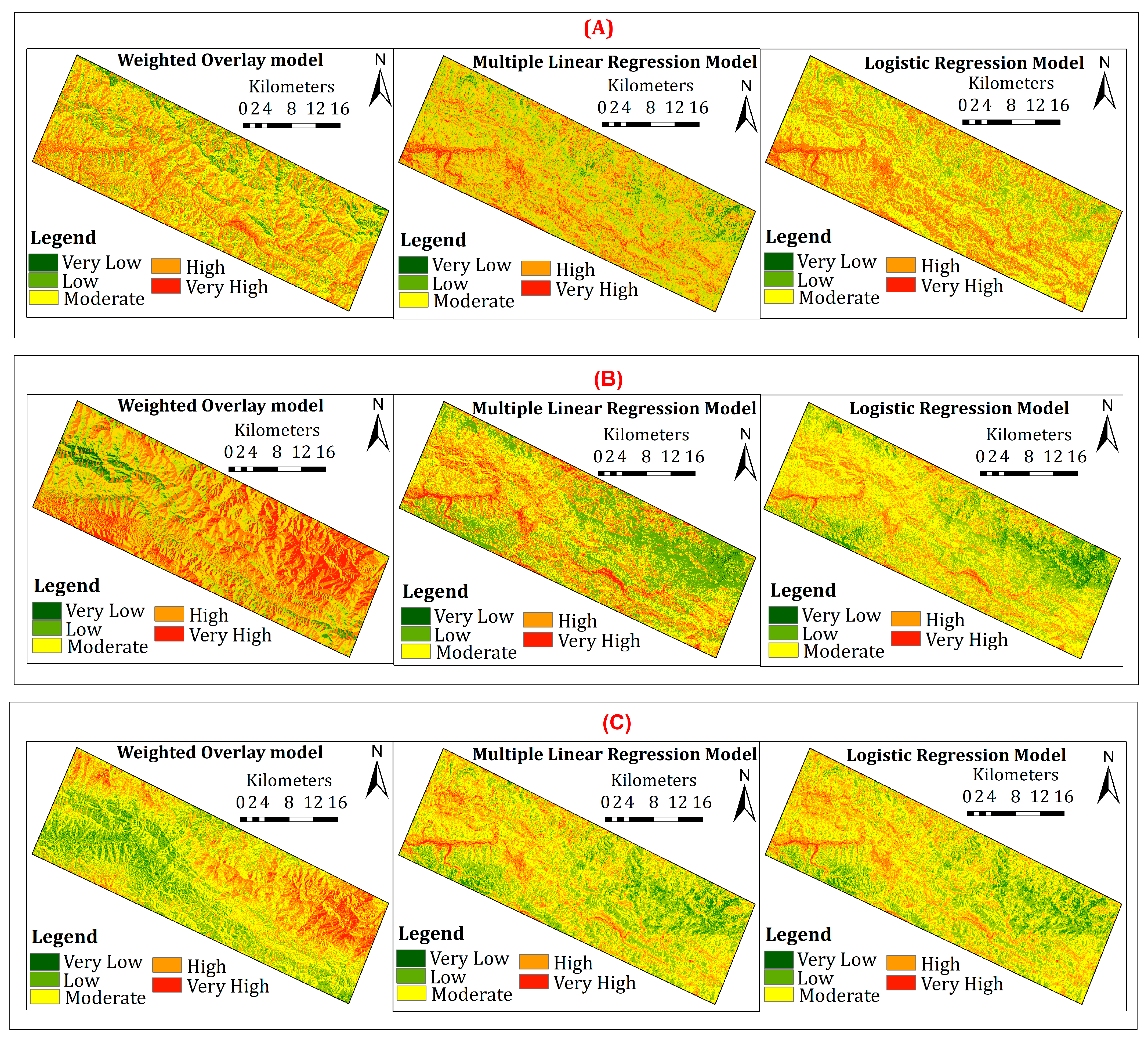
The correlation-based WO model combined NDBI, MNDVI, ARVI, TWI, SPI, and Aspect. The VIF and IG analyses produced different factors. However, the model’s essential structure remained consistent. Figure 6 shows LSMs prepared by WO, MLR, and LR methods with all three feature selection techniques. Different amounts of susceptibility classes, i.e., Very-High, High, Moderate, Low, and Very-Low can be seen in each case of modeling and feature selection. Continuous susceptibility indices (0–1) were classified into these five classes using the quantile (equal-frequency) method, which ensures each class contains an approximately equal number of pixels. This approach is widely used in susceptibility mapping to support balanced visual interpretation and comparison across models, while also reducing recall or high detection rates to extreme index values.
Moreover, several statistical measures were conducted in this study. We used these measures to establish the best performing model (Table 3 and Table 4) based on the LSMs generated by all models with different screening cases. The subsequent section describes these statistical measures in detail.
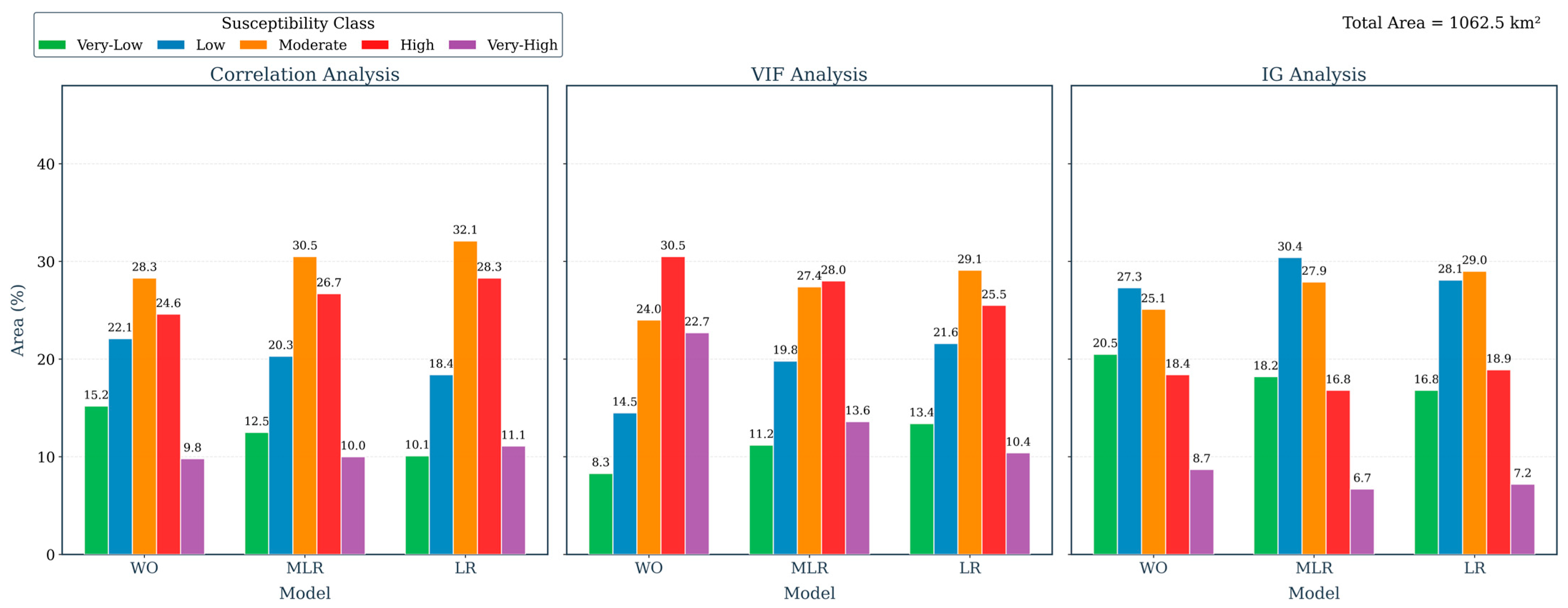
The spatial patterns depicted in the LSMs generated with Correlation Analysis (Figure 6A), VIF analysis (Figure 6B), and IG analysis (Figure 6C) were quantitatively assessed by calculating the areal percentage of each susceptibility class across 1062.5 km2 of the study area, as shown in Figure 7. The Correlation Analysis-based LR model, which visually exhibits balanced susceptibility zoning, allocated the largest proportion of the area to Moderate (32.1%) and High (28.3%) classes, reflecting its capacity to delineate intermediate-risk zones without overpredicting extremes. Conversely, the VIF analysis-based WO model, characterized by extensive high-susceptibility patches, assigned the highest percentages to High (30.5%) and Very-High (22.7%) classes, consistent with its high-recall, low-precision profile noted in Section 3.3 (Accuracy Assessment) below. IG analysis-based models, particularly IG-MLR and IG-LR, demonstrated a conservative risk allocation, with the greatest area concentrated in Low (30.4%) and Moderate (27.9%) classes, supporting their role as stable, regionally focused assessment tools (Figure 7). These areal distributions provide a quantitative foundation for the visual interpretations of Figure 6 and reinforce the performance metrics, as reported in Table 3, clarifying how each feature-selection method shapes the spatial expression of landslide susceptibility.

3.3. Accuracy Assessment

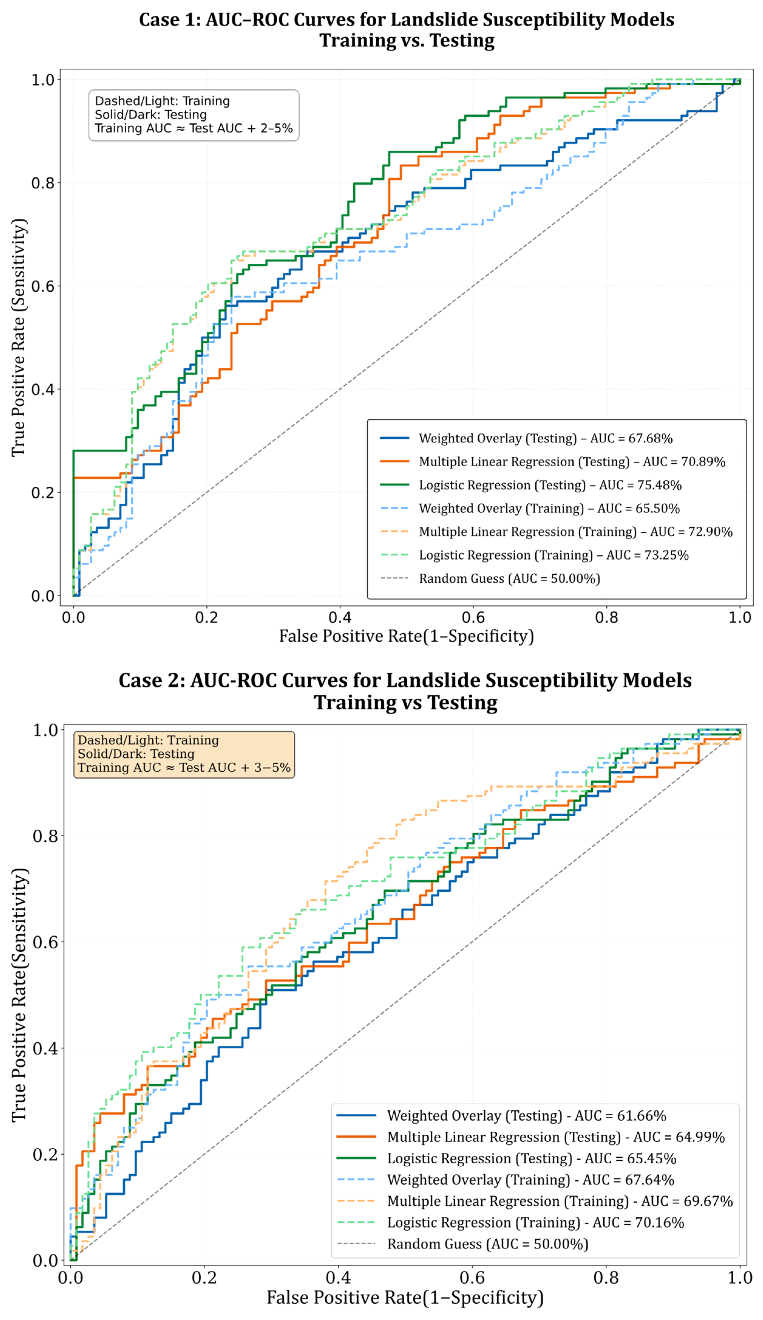
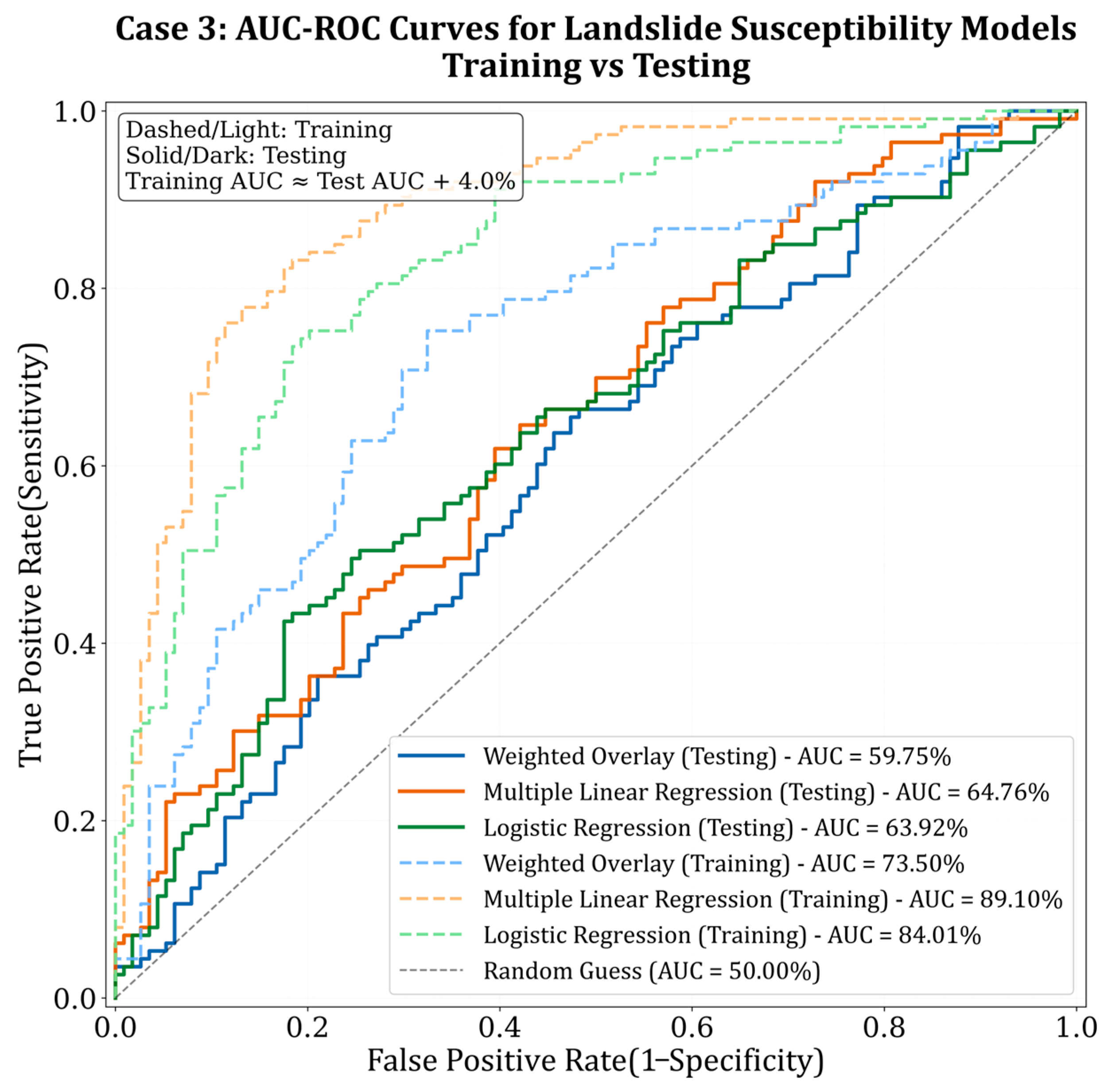
Referring to Figure 6, among the generated LSMs, the LR model with Correlation Analysis (Case 1) appears to be the most statistically valid result (Figure 8). This model has an accuracy of 69.30%, a precision of 64.47%, and a recall of 85.96% (refer to Table 3). These metrics produce a primary F1-score of 0.74. It shows an exceptional AUC-ROC score of 75.48%. Its prediction range is 0.06 to 1.00, with a mean prediction score of 0.67 (refer to Table 3). The LR model effectively balances risk detection and error prevention. This balance makes it an excellent tool for complete landslide risk evaluation. The correlation-LR combination demonstrated the best overall predictive performance, achieving the highest AUC-ROC (75.48%) and balanced accuracy (69.30%) as shown in Table 3, and effectively concentrated the highest density of known landslides in the Very High susceptibility class (Figure 9). This study further tested the robustness of the LR model. Additional experiments on different data splits confirmed their stable performance. An analysis of classification thresholds also clarifies its precision-recall trade-off.
The WO model with VIF analysis (Case 2) offers a different strength. It demonstrates a very high recall (true positive rate) of 90.18%. However, it has a lower precision of 58.72%. This high recall occurs because the WO model is a linear combination. The VIF-selected factors, like rainfall and MNDVI, receive high weights. This creates a sensitive model that flags most true landslides but also generates many false positives. The model has a restricted prediction range of 0.22 to 0.60 and a mean value of 0.40 (refer to Table 3).
The MLR model with IG analysis (Case 3) shows moderate performance. It has an accuracy of 62.11%, a precision of 60.15%, and a recall of 70.70%. These values result in an F1-score of 0.65. The model’s prediction range is 0.21 to 0.84, with a mean value of 0.50 (refer to Table 3). This distribution shows no systematic deviation. MLR serves as a dependable tool for regional mapping. It provides a safe and believable distribution of susceptibility, supported by an AUC-ROC of 64.76.
Spatial analysis of the landslide susceptibility maps reveals pronounced regional disparities in landslide susceptibility. A cross-model evaluation highlights distinct yet complementary behaviors under identical conditions. The landslide susceptibility maps derived from different methodologies were quantitatively compared by evaluating their predictive performance and analyzing the areal distribution across susceptibility classes (Figure 7). The LR model achieves reliable mean predictions in all cases. The WO model demonstrates the most restricted prediction ranges. It struggles to detect the full spectrum of susceptibility. The MLR model shows more stable performance metrics than the WO approach. In summary, each model serves a specific assessment purpose. The LR model with Correlation Analysis-based features proves the best overall predictive power. Its ability to model probability and capture non-linear thresholds, using a set of strong, non-redundant factors, enables nuanced, balanced performance. The WO model delivers the most sensitive detection performance while the MLR model provides reliable and consistent results.
Most importantly, the varying number of factors across methods (6 for Correlation Analysis, 8 for VIF, 12 for IG) means models were compared under unequal input dimensionality. This could influence performance, as more factors may provide richer information but also increase noise or overfitting. In the supplementary analysis with equalized factor count (top six factors per method), the correlation-LR combination still performed best. At the same time, VIF-WO retained high recall, and IG-MLR showed moderate accuracy (refer to Table 4). This suggests that the core conclusions regarding method suitability are robust despite dimensional differences. Nevertheless, practitioners should recognize that both selection logic and factor count jointly shaped model outcomes, and the choice of method should align with both statistical and practical mapping objectives.

3.4. Validation Robustness

A supplementary 5-fold spatial cross-validation, with folds defined by watershed sub-basins to ensure spatial independence, was conducted to assess the robustness of the model rankings. The results, as presented in Table 5, confirm that the performance trends remain stable and consistent with the primary 70/30 split evaluation. The correlation-based LR model consistently achieved the highest mean AUC and F1-score, while the VIF-based WO model maintained superior recall-oriented performance. Low standard deviations across all metrics indicate consistent model behavior under spatially independent validation, demonstrating that the primary findings are generalizable.
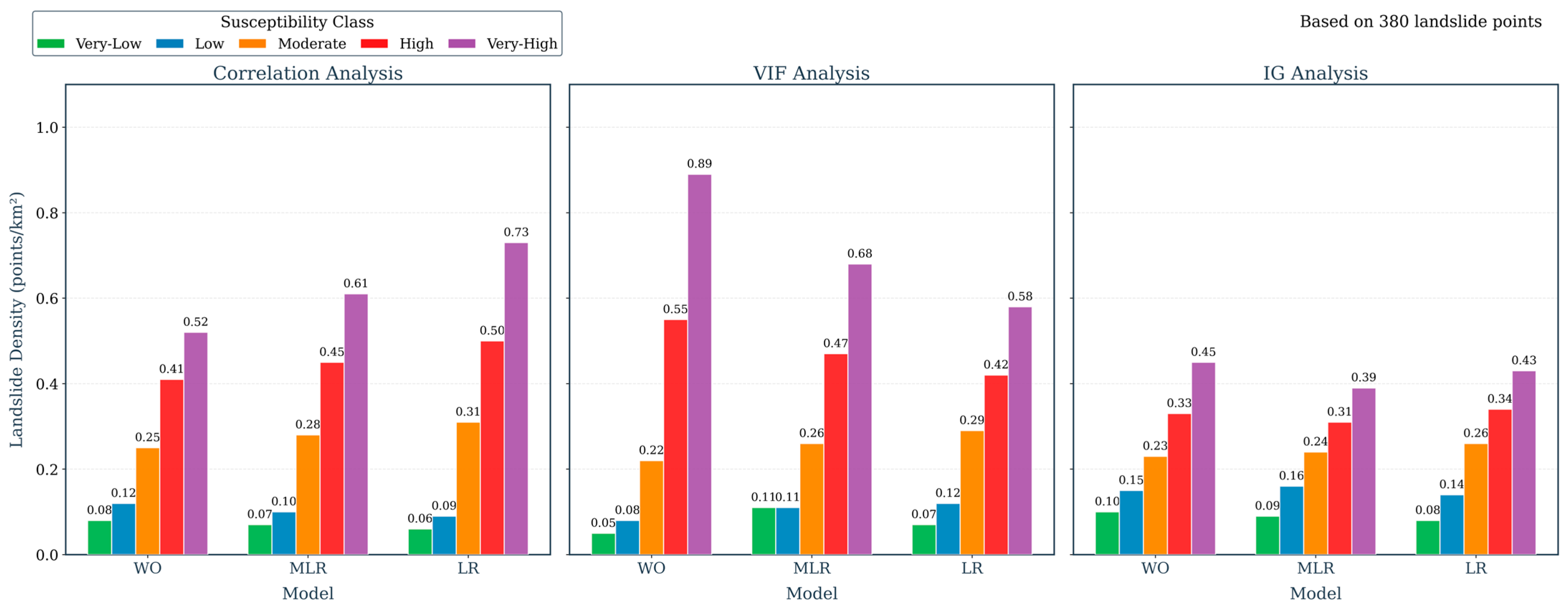
A comprehensive evaluation of the spatial predictive capability of each model, beyond conventional accuracy metrics, was conducted by analyzing the density of known landslide points within each predicted susceptibility class (Figure 9). This density analysis extends the areal distribution patterns observed in Figure 7, revealing how effectively each model concentrates actual landslides in predicted high-risk zones. The correlation-based LR model, which demonstrated balanced areal allocation in Figure 7, shows the strongest spatial discrimination, with landslide density increasing sharply from Very-Low (0.06 points/km2) to Very-High (0.73 points/km2) classes, confirming its superior ability to spatially align predictions with observed failures (Figure 9).
In contrast, the VIF-based WO model, noted for its high-risk areal emphasis, achieves the highest absolute density in the Very-High class (0.89 points/km2), supporting its high-recall design while explaining its lower precision due to over-prediction. IG-based models exhibit relatively flat density gradients (0.16–0.31 points/km2 across Low to High classes), consistent with their conservative risk allocation shown in Figure 6 and their role as stable regional assessment tools. Together, Figure 7 and Figure 9 provide complementary spatial validation: while Figure 7 quantifies each model’s inherent risk perception through areal distribution, Figure 8 validates how well that perception aligns with actual landslide occurrence, thereby strengthening the connection between susceptibility maps (Figure 6) and the performance metrics (Table 3).

4. Discussion

The systematic comparative assessment of feature selection techniques with traditional statistical models provided crucial insights into methodological requirements for effective LSM. This study highlights a persistent trade-off between maximizing statistical predictive performance and maintaining physical-mechanistic consistency, a necessary consideration for translating model results into practical hazard management [51,52].
The superior overall performance of the LR model optimized by Correlation Analysis (i.e., LR-Correlation model) validates a core premise of this study that features selection methods fundamentally shape model outcomes. This combination of success underscores the effectiveness of a selection strategy that balances statistical parsimony with physical interpretability for regional-scale mapping. Its statistically optimal metrics (e.g., AUC-ROC: 75.48%, Accuracy: 69.30%, Recall: 85.96%) demonstrate robust performance within an established modeling framework [53,54]. However, this statistical achievement is limited by a significant methodological limitation such as the emphasis of correlation-based approach on maximizing linear associations resulted in exclusion of geotechnically essential factors such as lithology and soil. While this exclusion is statistically justifiable for model fitting, it risks compromising the model ability to represent structural weakness and subsurface material properties [53,54], and is often inadequately characterized by coarse-resolution input data. As a result, the best statistical model may not fully capture the physical complexity inherent in the landslide process [55].
In contrast to the statistical optimum, the WO model with VIF analysis (WO-VIF) demonstrated the highest landslide detection capability with a recall of 90.18%. This method’s superior recall makes it exceptionally valuable in contexts of minimizing False Negatives (missed landslide events), which is critical [56,57], such as in emergency management and early warning systems. Conversely, the MLR with IG analysis (MLR-IG) offered a stable and balanced approach (Accuracy: 62.11%, AUC-ROC: 64.76%). These results indicate that the observed performance differences arise not merely from the selection strategies themselves but also from variations in input dimensionality and data richness among the resulting, non-uniform factor sets. This complexity offers a strictly methodological comparison challenging [58].
The systematic approach to factor selection employed in this study, balancing general physical principles, region-specific diagnostics, and data constraints, highlights a pathway to more reproducible LSM. The performance variations between models using different factor subsets (e.g., Correlation vs. VIF) underscore that the initial set of factors is as critical as the subsequent selection technique. The proposed framework (Mechanism, Diagnostic Value, Data Availability) offers practitioners a checklist to adapt this study rationale: first, include canonical factors (slope, lithology); second, incorporate locally diagnostic proxies (e.g., road density, specific weak rock units); and third, pragmatically adjust based on data quality. This moves beyond ad-hoc factor lists toward a principle-guided methodology that can be explicitly tailored and justified for new study areas.
A key limitation addressed by this study is that the evaluated feature selection methods (Correlation, VIF, and IG) are fundamentally a-spatial and non-geomorphic, focusing strictly on pairwise relationships and sample-level entropy reduction. They may overlook the critical influence of spatial autocorrelation and geomorphic continuity [59], both of which are fundamental characteristics of landslide processes [60]. Nevertheless, a vital check on physical plausibility across all models confirmed that the resulting high-susceptibility zones are consistently correlated with established preconditioning factors, namely steep slope gradients, hydrological convergence (high TWI values), and low vegetation cover [61,62], suggesting that statistical optimization did not lead to physically unreasonable results. To ensure the generalizability and robustness of the conclusions, a control analysis using a supplementary spatial cross-validation scheme was implemented [63], which further confirmed the stability of the reported model rankings and indicated limited overfitting.
The findings establish clear operational recommendations for comprehensive planning that prioritize predictive accuracy. The LR-Correlation model is best suited, while the WO-VIF method is recommended for emergency response planning due to its high detection recall. Future research must decisively address the persistent gap by integrating these statistically efficient, optimized models with mechanistic, physics-informed, or hybrid susceptibility frameworks [64,65]. This will be essential for moving beyond empirical performance comparisons toward a more mechanism-informed analysis. This ultimately enhances the physical interpretability and practical applicability of susceptibility assessments in mountainous environments.

5. Limitations/Challenges

5.1. Limitations Related to Input Data Accuracy and Resolution

The near-zero Pearson correlation observed for geology (Figure 5) led to its exclusion from the correlation-based LR model. This may reflect dataset limitations rather than the true insignificance of lithology. The 1:50,000-scale geological map, while regionally representative, may be too coarse to accurately delineate small but critical Quaternary sediment (Qs) deposits, such as those in the Bhimasthan area (~27°10′ N, 86°05′ E). This cartographic generalization is likely to contribute to mismatches between mapped Qs units and predicted high-susceptibility zones. Furthermore, the representation of major geological structures is based on regional 1:50,000 scale mapping. While verified with terrain models, the precise orientation and complexity of these structures at a local scale may vary from higher resolution tectonic interpretations.
Similarly, the SOTER soil database provides generalized classifications that may not capture local variations in soil thickness, texture, or hydraulic properties. These resolution and accuracy constraints highlight how traditional statistical models depend on input data quality [66]. Future studies would benefit from higher-resolution geological and soil mapping [67] or the integration of geotechnical field data to better represent subsurface controls on landslide initiation [68].

5.2. Temporal Consistency Between Inventory and Environmental Data

Lack of precise temporal alignment between the landslide inventory and dynamic environmental factors is another limitation of this study. The inventory spans 2015–2020, whereas factors such as mean annual rainfall and satellite-derived vegetation indices represent aggregated or snapshot conditions from a similar period, not necessarily coinciding with individual failure events. This indicates that the model is trained on representative rather than contemporaneous preconditioning factors, which may reduce accuracy for predicting landslides triggered by short-term events such as extreme storms [69]. Nevertheless, regional susceptibility mapping aimed at identifying spatially persistent predisposing conditions such as steep slopes, weak lithology, or generally high-rainfall areas, this approach remains valid and widely adopted. Future work could improve temporal accuracy by using event-dated inventories paired with antecedent rainfall data and pre-failure imagery [70,71].

6. Conclusions

This study presents a practical framework for landslide susceptibility model selection by systematically comparing three feature selection techniques: Correlation Analysis, Variance Inflation Factor (VIF), and Information Gain (IG), with three traditional modeling approaches: Weighted Overlay (WO), Multiple Linear Regression (MLR), and Logistic Regression (LR). For comprehensive landslide susceptibility mapping and regulatory planning, LR combined with Correlation Analysis produces the most statistically robust predictions, providing balanced performance metrics suitable for applications prioritizing predictive accuracy. However, this method preferentially selects linearly correlated variables, potentially underrepresenting non-linear or weakly correlated geotechnical factors.
For emergency response and early warning applications, the WO model incorporating VIF analysis demonstrates superior detection capability by maximizing recall, thereby minimizing overlooked landslides. Meanwhile, MLR with IG offers a stable and balanced approach for standardized regional assessments, making it suitable for conservative risk prioritization.
A key insight from this study is that statistical optimization does not necessarily ensure geomorphic realism. For instance, the Correlation Analysis-based LR model excludes lithology and soil despite their established role in slope stability, highlighting an inherent trade-off between predictive performance and physical representativeness. As a result, this study highlights the importance of complementing statistical model selection with domain expertise and field-based validation to ensure both high predictive accuracy and mechanistic credibility in practical applications.
The principal contribution of this study lies in its empirical comparison and the resulting operational guidelines, demonstrating the value of established feature selection techniques rather than proposing new algorithms. Future work should explore hybrid frameworks that integrate the statistical efficiency of optimized traditional models with the mechanistic transparency of physics-based approaches. Such integration would enhance both interpretability and applicability, especially in data-scarce mountainous regions, ultimately supporting more reliable and actionable landslide risk assessments.

Author Contributions

Data collection, data preparation, data management, methodology development, landslide susceptibility mapping and analysis, and manuscript draft preparation were all completed by Buddhi Raj Joshi, and Niraj K.C. contributed to the model verification, data updating, data verification, and draft improvement. The work was further conceptualized, and the paper was revised with feedback from Indra Prasad Acharya. Netra Prakash Bhandary supervised with overall oversight, modification, and finalization of the manuscript. All authors have read and agreed to the published version of the manuscript.

Funding

This research received no external funding.

Data Availability Statement

During the manuscript preparation, generative AI and AI-assisted technologies were also used for paraphrasing, grammar, and English editing to improve the readability of the work. After using the AI tools, the text was reviewed and edited by all authors as and when required. The authors take full responsibility for the published content, including all ideas, concepts, insights, scientific conclusions, and recommendations.

Acknowledgments

The first author is grateful for the resources and support from Ehime University, Japan, Pokhara University, Nepal, and Japan Society of Promotion of Science (JSPS). All authors acknowledge all data sources such as Google Earth, SOTER Database for Nepal, the Department of Mines and Geology of Nepal, CHIRPS (Climate Hazards Group Infrared Precipitation Station) and the European Space Agency for providing crucial data sets like ASTER DEM, and Sentinel-2A datasets for a successful run of this study.

Conflicts of Interest

The authors declare no conflict of interest.

References

  1. Niraj, K.C.; Singh, A.; Shukla, D.P. Effect of the normalized difference vegetation index (NDVI) on GIS-enabled bivariate and multivariate statistical models for landslide susceptibility mapping. J. Indian Soc. Remote Sens. 2023, 51, 1739–1756. [Google Scholar] [CrossRef]
  2. Haque, U.; Blum, P.; da Silva, P.F.; Andersen, P.; Pilz, J.; Chalov, S.R.; Malet, J.-P.; Auflič, M.J.; Andres, N.; Poyiadji, E.; et al. Fatal landslides in Europe. Landslides 2016, 13, 1545–1554. [Google Scholar] [CrossRef]
  3. Felicísimo, Á.M.; Cuartero, A.; Remondo, J.; Quirós, E. Mapping landslide susceptibility with logistic regression, multiple adaptive regression splines, classification and regression trees, and maximum entropy methods: A comparative study. Landslides 2013, 10, 175–189. [Google Scholar] [CrossRef]
  4. Chen, T.; Niu, R.; Jia, X. A comparison of information value and logistic regression models in landslide susceptibility mapping by using GIS. Environ. Earth Sci. 2016, 75, 867. [Google Scholar] [CrossRef]
  5. Singh, A.; Chhetri, N.K.; Dhiman, N.; Gupta, S.K.; Shukla, D.P. Strategies for sampling pseudo-absences of landslide locations for landslide susceptibility mapping in complex mountainous terrain of Northwest Himalaya. Bull. Eng. Geol. Environ. 2023, 82, 321. [Google Scholar] [CrossRef]
  6. Niraj, K.C.; Singh, A.; Shukla, D.P. Improved Landslide Susceptibility mapping using statistical MLR model. In Proceedings of the 2023 International Conference on Machine Intelligence for GeoAnalytics and Remote Sensing (MIGARS), Hyderabad, India, 27–29 January 2023; IEEE: New York, NY, USA, 2023; Volume 1, pp. 1–4. [Google Scholar] [CrossRef]
  7. Huang, F.; Ye, Z.; Jiang, S.-H.; Huang, J.; Chang, Z.; Chen, J. Uncertainty study of landslide susceptibility prediction considering the different attribute interval numbers of environmental factors and different data-based models. Catena 2021, 202, 105250. [Google Scholar] [CrossRef]
  8. Brenning, A. Spatial prediction models for landslide hazards: Review, comparison, and evaluation. Nat. Hazards Earth Syst. Sci. 2005, 5, 853–862. [Google Scholar] [CrossRef]
  9. Gupta, S.K.; Shukla, D.P. Effect of scale and mapping unit on landslide susceptibility mapping of Mandakini River Basin, Uttarakhand, India. Environ. Earth Sci. 2022, 81, 373. [Google Scholar] [CrossRef]
  10. Singh, A.; Dhiman, N.; KC, N.; Shukla, D.P. Improving ML-based landslide susceptibility using ensemble method for sample selection: A case study of Kangra district in Himachal Pradesh, India. Environ. Sci. Pollut. Res. 2024, 1–24. [Google Scholar] [CrossRef]
  11. Yang, Y.; Ji, F.; Gao, Y.; Liang, P. Slope Stability Analysis Using a Surrogate Model with Varying Sampling Precision: A Case Study of Open-Pit Mine Dump Slopes. Nat. Hazards 2025, 121, 10963–10988. [Google Scholar] [CrossRef]
  12. Azmoon, B.; Biniyaz, A.; Liu, Z. Use of High-Resolution Multi-Temporal DEM Data for Landslide Detection. Geosciences 2022, 12, 378. [Google Scholar] [CrossRef]
  13. Lari, S.; Frattini, P.; Crosta, G.B. A Probabilistic Approach for Landslide Hazard Analysis. Eng. Geol. 2014, 182, 3–14. [Google Scholar] [CrossRef]
  14. Alvioli, M.; Marchesini, I.; Reichenbach, P.; Rossi, M.; Ardizzone, F.; Fiorucci, F.; Guzzetti, F. Automatic delineation of geomorphological slope units with r.slopeunits v1.0 and their optimization for landslide susceptibility modeling. Geosci. Model Dev. 2016, 9, 3975–3991. [Google Scholar] [CrossRef]
  15. Reichenbach, P.; Rossi, M.; Malamud, B.D.; Mihir, M.; Guzzetti, F. A review of statistically based landslide susceptibility models. Earth-Sci. Rev. 2018, 180, 60–91. [Google Scholar] [CrossRef]
  16. Pudasaini, S.P.; Mergili, M. A multi-phase mass flow model. J. Geophys. Res. Earth Surf. 2019, 124, 2920–2942. [Google Scholar] [CrossRef]
  17. Chen, W.; Peng, J.; Hong, H.; Shahabi, H.; Pradhan, B.; Liu, J.; Zhu, A.-X.; Pei, X.; Duan, Z. Landslide susceptibility modelling using GIS-based machine learning techniques for Chongren County, Jiangxi Province, China. Sci. Total Environ. 2018, 626, 1121–1135. [Google Scholar] [CrossRef] [PubMed]
  18. Li, X.; Chong, J.; Lu, Y.; Li, Z. Application of information gain in the selection of factors for regional slope stability evaluation. Bull. Eng. Geol. Environ. 2022, 81, 470. [Google Scholar] [CrossRef]
  19. Chen, C.Y.; Chang, J.M. Landslide dam formation susceptibility analysis based on geomorphic features. Landslides 2016, 13, 1019–1033. [Google Scholar] [CrossRef]
  20. Abedini, M.; Ghasemian, B.; Shirzadi, A.; Bui, D.T. A comparative study of support vector machine and logistic model tree classifiers for shallow landslide susceptibility modeling. Environ. Earth Sci. 2019, 78, 560. [Google Scholar] [CrossRef]
  21. Du, G.L.; Zhang, Y.S.; Iqbal, J.; Yang, Z.H.; Yao, X. Landslide susceptibility mapping using an integrated model of information value method and logistic regression in the Bailongjiang watershed, Gansu Province, China. J. Mt. Sci. 2017, 14, 249–268. [Google Scholar] [CrossRef]
  22. Huang, S.; Chen, L. Landslide susceptibility mapping using an integration of different statistical models for the 2015 Nepal earthquake in Tibet. Geomat. Nat. Hazards Risk 2024, 15, 2396908. [Google Scholar] [CrossRef]
  23. Harvey, N.; Razavi, S.; Bilish, S. Review of hydrological modelling in the Australian Alps: From rainfall-runoff to physically based models. Australas. J. Water Resour. 2024, 28, 208–224. [Google Scholar] [CrossRef]
  24. Kucklick, J.-P.; Müller, O. Tackling the Accuracy-Interpretability Trade-Off: Interpretable Deep Learning Models for Satellite Image-Based Real Estate Appraisal. ACM Trans. Manag. Inf. Syst. 2023, 14, 1–24. [Google Scholar] [CrossRef]
  25. Kumar, C.; Walton, G.; Santi, P.; Luza, C. An ensemble approach of feature selection and machine learning models for regional landslide susceptibility mapping in the arid mountainous terrain of Southern Peru. Remote Sens. 2023, 15, 1376. [Google Scholar] [CrossRef]
  26. Aristizábal-Giraldo, E.V.; Vélez-Upegui, J.I.; Martínez-Carvajal, H.E. A Comparison of Linear and Nonlinear Model Perfor-mance of SHIA_Landslide: A Forecasting Model for Rainfall-Induced Landslides. Rev. Fac. Ing. Univ. Antioq. 2016, 80, 74–88. [Google Scholar] [CrossRef]
  27. Sah, R.B.; Paudyal, K.R. Geological control of mineral deposits in Nepal. J. Nepal Geol. Soc. 2019, 58, 189–197. [Google Scholar] [CrossRef]
  28. Riesner, M.; Bollinger, L.; Rizza, M.; Klinger, Y.; Karakaş, Ç.; Sapkota, S.N.; Shah, C.; Guérin, C.; Tapponnier, P. Surface rupture and landscape response in the middle of the great Mw 8.3 1934 earthquake mesoseismal area: Khutti Khola site. Sci. Rep. 2023, 13, 4566. [Google Scholar] [CrossRef]
  29. Wikipedia Contributors. Sindhuli District. Wikipedia, the Free Encyclopedia. Available online: https://en.wikipe-dia.org/wiki/Sindhuli_District (accessed on 1 October 2025).
  30. Kaufman, Y.J.; Tanre, D. Atmospherically resistant vegetation index (ARVI) for EOS-MODIS. IEEE Trans. Geosci. Remote Sens. 1992, 30, 261–270. [Google Scholar] [CrossRef]
  31. Wang, S.H.; Sun, W.; Li, S.W.; Shen, Z.X.; Fu, G. Interannual variation of the growing season maximum normalized difference vegetation index, MNDVI, and its relationship with climatic factors on the Tibetan Plateau. Pol. J. Ecol. 2015, 63, 424–439. [Google Scholar] [CrossRef]
  32. Guha, S.; Govil, H.; Dey, A.; Gill, N. Analytical study of land surface temperature with NDVI and NDBI using Landsat 8 OLI and TIRS data in Florence and Naples city, Italy. Eur. J. Remote Sens. 2018, 51, 667–678. [Google Scholar] [CrossRef]
  33. Funk, C.; Peterson, P.; Landsfeld, M.; Pedreros, D.; Verdin, J.; Shukla, S.; Husak, G.; Rowland, J.; Harrison, L.; Hoell, A.; et al. The climate hazards infrared precipitation with stations—A new environmental record for monitoring extremes. Sci. Data 2015, 2, 150066. [Google Scholar] [CrossRef] [PubMed]
  34. Food and Agriculture Organization of the United Nations. The Soil and Terrain Database for Nepal (SOTER) (1:1,000,000 Scale) [Data Set]. 1995. Available online: http://www.fao.org/soils-portal/soil-survey/soil-maps-and-databases/harmonized-world-soil-database-v12/en/ (accessed on 15 December 2025).
  35. Department of Mines and Geology. General Geology (Government of Nepal). 2023. Available online: https://dmgnepal.gov.np/en/pages/general-geology-4128. (accessed on 18 December 2025).
  36. OpenStreetMap Contributors. OpenStreetMap [Data set]. 2020. Available online: https://www.openstreetmap.org (accessed on 18 December 2025).
  37. Jones, K.H. A comparison of algorithms used to compute hill slope as a property of the DEM. Comput. Geosci. 1998, 24, 315–323. [Google Scholar] [CrossRef]
  38. Jurgens, C. The modified normalized difference vegetation index (MNDVI) a new index to determine frost damages in agriculture based on Landsat TM data. Int. J. Remote Sens. 1997, 18, 3583–3594. [Google Scholar] [CrossRef]
  39. Miura, T.; Huete, A.R.; Yoshioka, H.; Holben, B.N. An error and sensitivity analysis of atmospheric resistant vegetation indices derived from dark target-based atmospheric correction. Remote Sens. Environ. 2001, 78, 284–298. [Google Scholar] [CrossRef]
  40. Zha, Y.; Gao, J.; Ni, S. Use of normalized difference built-up index in automatically mapping urban areas from TM imagery. Int. J. Remote Sens. 2003, 24, 583–594. [Google Scholar] [CrossRef]
  41. Sedgwick, P. Pearson’s correlation coefficient. BMJ 2012, 345, e4483. [Google Scholar] [CrossRef]
  42. Puth, M.T.; Neuhäuser, M.; Ruxton, G.D. Effective use of Spearman’s and Kendall’s correlation coefficients for association between two measured traits. Anim. Behav. 2015, 102, 77–84. [Google Scholar] [CrossRef]
  43. Gupta, S.D. Point biserial correlation coefficient and its generalization. Psychometrika 1960, 25, 393–408. [Google Scholar] [CrossRef]
  44. Juliev, M.; Mergili, M.; Mondal, I.; Nurtaev, B.; Pulatov, A.; Hübl, J. Comparative analysis of statistical methods for landslide susceptibility mapping in the Bostanlik District, Uzbekistan. Sci. Total Environ. 2019, 653, 801–814. [Google Scholar] [CrossRef]
  45. Panahi, M.; Rezaie, F.; Khosravi, K.; Kalantari, Z.; Bateni, S.M.; Lee, J.A. Beyond boundaries: AI-optimized global landslide susceptibility mapping. Geomat. Nat. Hazards Risk 2025, 16, 2493222. [Google Scholar] [CrossRef]
  46. Awawdeh, M.M.; ElMughrabi, M.A.; Atallah, M.Y. Landslide susceptibility mapping using GIS and weighted overlay method: A case study from North Jordan. Environ. Earth Sci. 2018, 77, 732. [Google Scholar] [CrossRef]
  47. Bravo-López, E.; Fernández Del Castillo, T.; Sellers, C.; Delgado-García, J. Landslide Susceptibility Mapping of Landslides with Artificial Neural Networks: Multi-Approach Analysis of Backpropagation Algorithm Applying the Neuralnet Package in Cuenca, Ecuador. Remote Sens. 2022, 14, 3495. [Google Scholar] [CrossRef]
  48. Costache, R.; Ali, S.A.; Parvin, F.; Pham, Q.B.; Arabameri, A.; Nguyen, H.; Crăciun, A.; Anh, D.T. Detection of areas prone to flood-induced landslides risk using certainty factor and its hybridization with FAHP, XGBoost and deep learning neural net-work. Geocarto Int. 2022, 37, 7303–7338. [Google Scholar] [CrossRef]
  49. Khaliq, A.H.; Basharat, M.; Riaz, M.T.; Riaz, M.T.; Wani, S.; Al-Ansari, N.; Le, L.B.; Linh, N.T.T. Spatiotemporal landslide susceptibility mapping using machine learning models: A case study from district Hattian Bala, NW Himalaya, Pakistan. Ain Shams Eng. J. 2023, 14, 101907. [Google Scholar] [CrossRef]
  50. Zeng, G. Invariance Properties and Evaluation Metrics Derived from the Confusion Matrix in Multiclass Classification. Mathematics 2025, 13, 2609. [Google Scholar] [CrossRef]
  51. Tehrani, F.S.; Calvello, M.; Liu, Z.; Zhang, L.; Lacasse, S. Machine learning and landslide studies: Recent advances and applications. Nat. Hazards 2022, 114, 1197–1245. [Google Scholar] [CrossRef]
  52. Zimmaro, P.; Ausilio, E. Numerical evaluation of natural periods and mode shapes of earth dams for probabilistic seismic hazard analysis applications. Geosciences 2020, 10, 499. [Google Scholar] [CrossRef]
  53. Gray, J.M.; Bishop, T.F.; Wilford, J.R. Lithology and soil relationships for soil modelling and mapping. Catena 2016, 147, 429–440. [Google Scholar] [CrossRef]
  54. Van Westen, C.J. The modelling of landslide hazards using GIS. Surv. Geophys. 2000, 21, 241–255. [Google Scholar] [CrossRef]
  55. Varnes, D.J. Landslide Hazard Zonation: A Review of Principles and Practice (No. 3). 1984. Available online: http://worldcat.org/isbn/9231018957 (accessed on 25 December 2025).
  56. Tien Bui, D.; Tuan, T.A.; Klempe, H.; Pradhan, B.; Revhaug, I. Spatial prediction models for shallow landslide hazards: A comparative assessment of the efficacy of support vector machines, artificial neural networks, kernel logistic regression, and logistic model tree. Landslides 2016, 13, 361–378. [Google Scholar] [CrossRef]
  57. Mondini, A.C.; Guzzetti, F.; Melillo, M. Deep learning forecast of rainfall-induced shallow landslides. Nat. Commun. 2023, 14, 2466. [Google Scholar] [CrossRef]
  58. Magar, T.A.; Bhandari, B.P. Application of the bivariate frequency ratio method for landslide susceptibility mapping of Manthali Municipality, Ramechhap District, Nepal. Nepal J. Environ. Sci. 2025, 13, 43–60. [Google Scholar] [CrossRef]
  59. de Lara Maia, A.C.; Ayres, A.L.d.S.M.; Kanai, C.S.; da Silva Ferreira, J.; Fontes, M.R.; Desani, N.M.; Guimarães, Y.C.; de Praga Baião, C.F.; Mantovani, J.R.; Nery, T.D.; et al. Scale-Dependent Controls on Landslide Susceptibility in Angra dos Reis (Brazil) Revealed by Spatial Regression and Autocorrelation Analyses. Geomatics 2025, 5, 49. [Google Scholar] [CrossRef]
  60. Malamud, B.D.; Turcotte, D.L.; Guzzetti, F.; Reichenbach, P. Landslide inventories and their statistical properties. Earth Surf. Process. Landf. 2004, 29, 687–711. [Google Scholar] [CrossRef]
  61. Dai, F.C.; Lee, C.F.; Wang, S.J. Characterization of rainfall-induced landslides. Int. J. Remote Sens. 2003, 24, 4817–4834. [Google Scholar] [CrossRef]
  62. Chen, W.; Shirzadi, A.; Shahabi, H.; Ahmad, B.B.; Zhang, S.; Hong, H.; Zhang, N. A novel hybrid artificial intelligence approach based on the rotation forest ensemble and naïve Bayes tree classifiers for a landslide susceptibility assessment in Langao County, China. Geomat. Nat. Hazards Risk 2017, 8, 1955–1977. [Google Scholar] [CrossRef]
  63. Brenning, A. Spatial cross-validation and bootstrap for the assessment of prediction rules in remote sensing: The R package sperrorest. In Proceedings of the 2012 IEEE International Geoscience and Remote Sensing Symposium, Munich, Germany, 22–27 July 2012; pp. 5372–5375. [Google Scholar] [CrossRef]
  64. Ye, C.; Wu, H.; Oguchi, T.; Tang, Y.; Pei, X.; Wu, Y. Physically Based and Data-Driven Models for Landslide Susceptibility Assessment: Principles, Applications, and Challenges. Remote Sens. 2025, 17, 2280. [Google Scholar] [CrossRef]
  65. Cui, H.; Ji, J.; Hürlimann, M.; Medina, V. Probabilistic and physically-based modelling of rainfall-induced landslide susceptibility using integrated GIS-FORM algorithm. Landslides 2024, 21, 1461–1481. [Google Scholar] [CrossRef]
  66. Remondo, J.; González-Díez, A.; De Terán, J.R.D.; Cendrero, A. Landslide susceptibility models utilising spatial data analysis techniques. A case study from the lower Deba Valley, Guipúzcoa (Spain). Nat. Hazards 2003, 30, 267–279. [Google Scholar] [CrossRef]
  67. Lee, S.; Choi, J.; Woo, I. The effect of spatial resolution on the accuracy of landslide susceptibility mapping: A case study in Boun, Korea. Geosci. J. 2004, 8, 51–60. [Google Scholar] [CrossRef]
  68. Woodard, J.B.; Mirus, B.B. Overcoming the data limitations in landslide susceptibility modeling. Sci. Adv. 2025, 11, eadt1541. [Google Scholar] [CrossRef] [PubMed]
  69. Petley, D. Global patterns of loss of life from landslides. Geology 2012, 40, 927–930. [Google Scholar] [CrossRef]
  70. Kim, S.W.; Chun, K.W.; Kim, M.; Catani, F.; Choi, B.; Seo, J.I. Effect of antecedent rainfall conditions and their variations on shallow landslide-triggering rainfall thresholds in South Korea. Landslides 2021, 18, 569–582. [Google Scholar] [CrossRef]
  71. Kirschbaum, D.; Stanley, T.; Zhou, Y. Spatial and temporal analysis of a global landslide catalog. Geomorphology 2015, 249, 4–15. [Google Scholar] [CrossRef]
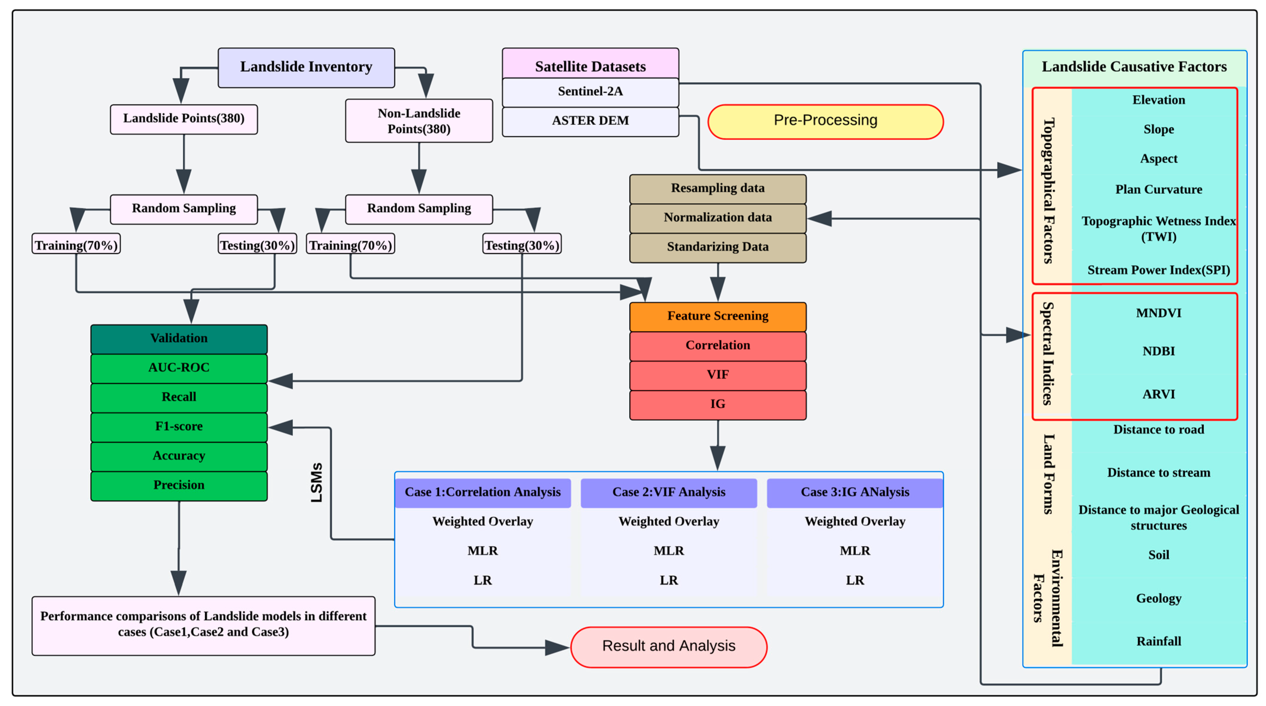
Figure 2. Methodological workflow for comparative landslide susceptibility assessment. (Note: The boxes represent process stages and data, the arrows indicate the sequential flow, and the colors distinguish the methodological stages; the data sources, sampling/preprocessing, feature screening, modeling, and validation/output).
Ijgi 15 00020 g002
Figure 3. Normalized landslide causative factor maps (values 0–1) with landslide and non-landslide sample locations: (A) Elevation, (B) Slope, (C) Aspect, (D) Curvature, (E) TWI, (F) SPI, (G) Distance to River, (H) Geology, (I) Soil, (J) Distance to Road, (K) NDBI, (L) Rainfall, (M) MNDVI, (N) Atmospherically Resistant Vegetation Index (ARVI), (O) Distance to Major Geological Structures.
Ijgi 15 00020 g003
Figure 4. Statistical comparison of landslide causative factors (on the horizontal axis) between landslide (LS) and non-landslide (NLS) areas.
Ijgi 15 00020 g004
Figure 5. Comparative assessment of feature selection techniques for landslide susceptibility mapping: (A) Correlation Analysis showing absolute Pearson coefficients coefficient for all 15 causative factors (green: p < 0.01; red: p ≥ 0.05); selected factors (p < 0.01) marked with ★ and weights (w), (B) Multicollinearity analysis using Variance Inflation Factor (VIF); factors with VIF < 2 (blue) selected, (C) Information Gain (IG) analysis; factors with IG > 0.4 (green) selected, and (D) Selection matrix comparing factor inclusion across methods; green squares indicate selection.
Ijgi 15 00020 g005
Figure 6. LSMs generated by using WO, MLR, LR models with the three feature selection techniques: (A) Correlation Analysis, (B) Variance Inflation Factor (VIF) Analysis, and (C) Information Gain (IG) Analysis.
Ijgi 15 00020 g006
Figure 7. Areal distribution of landslide susceptibility classes obtained from the three models (i.e., WO, MLR, and LR; on the horizontal axis) in combination with three feature selection methods (i.e., Correlation Analysis, VIF analysis, and IG analysis); the bar charts show the percentage of total study area (1062.5 km2) in each susceptibility class for each model with each feature selection technique; the WO-VIF model emphasizes high risk zones, LR-Correlation model yields balanced distribution, and IG-based models show conservative risk allocation.
Ijgi 15 00020 g007
Figure 8. Performance comparison of the LSMs generated by WO, MLR, and LR models on training vs. testing data; AUC-ROC curves for the three cases show a clear progression from high overfitting in Case 1 (models perform poorly on new data) to strong generalization and high accuracy in Case 3 (models are reliable for real-world prediction.
Ijgi 15 00020 g008aIjgi 15 00020 g008b
Figure 9. Landslide point density in each susceptibility class obtained from the susceptibility models and feature selection techniques; the LR-correlation model shows the strongest discrimination (0.06 to 0.73 landslides/km2), confirming superior spatial predictive capability, WO-VIF model yields the highest density in Very-High class (0.89/km2), supporting its high-recall design, and IG models result in flatter gradients, consistent with conservative risk allocation.
Ijgi 15 00020 g009
Table 1. Descriptive landslide causative factors used in the landslide susceptibility mapping, including their units, ranges, classifications, and a new column detailing the primary selection justification based on the framework of mechanism, diagnostic value, and data availability.
Causative
Factors
UnitRange/ClassesDescriptionSelection
Justification
Elevationmeters (m)1910 to 2280Height above sea level influencing slope stabilityCore Geomorphic
Slopedegrees (°)0 to 61.78Steepness of terrain affecting landslide probabilityCore Geomorphic [37]
Aspectdegrees (°)−1 to 359.79Direction of slope face affecting soil moisture & erosionCore Geomorphic
Curvature−3.61 (concave) to 2.83 (convex)Terrain curvature influencing water flow convergence/divergenceCore Geomorphic
TWI2.69 to 23.01Predicts soil moisture accumulation based on slope and upslope areaMechanistic (Hydrologic) [38]
SPI−13.82 to 12.15Estimates erosive power of streams based on slope and flow accumulationMechanistic (Hydrologic)
Distance to Rivermeters (m)0 to 1623.61Proximity to rivers affecting erosion and saturationRegional Diagnostic [21]
GeologyBh, OGR, Na, Qs, SiRock types and their susceptibility to weathering/erosionRegional Diagnostic [27,28]
Soil TypesPHh, RGd, CMe, CMgSoil properties influencing water retention and slope stabilityData-Constrained
Distance to Roadmeters (m)0 to 13,606.1Human-induced destabilization due to constructionAnthropogenic Proxy [21,29]
NDBI−0.53 to 0.29Indicates urbanization impact on land stabilityAnthropogenic Proxy
Rainfallmillimeters (mm)1223.05 to 1575.3Precipitation intensity affecting soil saturationMechanistic (Trigger)
MNDVI−0.066 to 0.92Vegetation cover density influencing slope reinforcementCore Geomorphic
ARVI−0.07 to 0.92Vegetation measure adjusted for atmospheric effectsCore Geomorphic
Distance to Major Geological Structuresmeters (m)0 to 12,063.7Proximity to mapped faults and thrusts, representing zones of structural weakness, groundwater movement, and reduced shear strengthRegional Diagnostic
Table 2. Statistical summary of landslide proximity to anthropogenic and fluvial features.
Proximity Zone (Meters)Distance to RoadsDistance to Rivers
0–5001668 (78% of total)1604 (75% of total)
500–1000257 (12% of total)321 (15% of total)
1000–2000139 (7% of total)214 (10% of total)
2000–500075 (3% of total)0 (0% of total)
>50000 (0% of total)0 (0% of total)
Total Landslides2139 (100%)2139 (100%)
Table 3. Model performance metrics; AUC-ROC, Accuracy, Precision, Recall, F1-score, Prediction Range, and Mean Prediction Value for the three models; WO, MLR, and LR with the three feature selection techniques.
ModelAUC-ROC (%)Accuracy (%)Precision (%)Recall (%)F1-ScorePrediction RangeMean Prediction Value
Case 1: Correlation Analysis
WO67.6866.6771.1156.140.62750.18–0.820.48
MLR70.8967.1162.9183.330.7170.25–0.900.62
LR75.4869.364.4785.960.73680.06–1.000.67
Case 2: VIF analysis
WO61.6663.5658.7290.180.71130.22–0.600.4
MLR64.9964.0060.4080.360.68970.30–0.780.53
LR65.4564.0063.4865.180.64320.28–0.850.55
Case 3: IG analysis
WO59.7557.7166.0453.970.52170.15–0.700.38
MLR64.7662.1160.1570.70.65040.21–0.840.5
LR63.9264.7667.0157.520.6190.20–0.800.49
Table 4. Model performance using the top six factors selected by each method (equal dimensionality control).
MethodModelAUC-ROC (%)Accuracy (%)F1-Score
Correlation Analysis (top 6)WO67.6866.670.63
MLR70.8967.110.72
LR75.4869.30.74
VIF Analysis (top 6)WO60.8862.340.7
MLR64.2163.450.68
LR64.8763.120.64
IG Analysis (top 6)WO59.3256.780.52
MLR63.4561.230.65
LR62.8963.450.61
Table 5. Performance metrics (mean ± one standard deviation) from 5-fold spatial cross-validation.
Model + Feature SelectionMean AUC (±Std)Mean Accuracy (±Std)Mean F1-Score (±Std)
LR + Correlation0.745 (±0.018)0.688 (±0.015)0.728 (±0.012)
WO + VIF0.608 (±0.022)0.621 (±0.019)0.705 (±0.017)
MLR + IG0.638 (±0.016)0.615 (±0.014)0.642 (±0.011)
LR + IG0.630 (±0.020)0.628 (±0.018)0.612 (±0.015)
WO + Correlation0.665 (±0.017)0.658 (±0.015)0.620 (±0.013)
MLR + VIF0.640 (±0.019)0.625 (±0.016)0.682 (±0.014)
Disclaimer/Publisher’s Note: The statements, opinions and data contained in all publications are solely those of the individual author(s) and contributor(s) and not of MDPI and/or the editor(s). MDPI and/or the editor(s) disclaim responsibility for any injury to people or property resulting from any ideas, methods, instructions or products referred to in the content.