Abstract
Normal faults play a key role in accommodating extensional deformation within the South Tibet Rift. The MS 6.8 Tingri earthquake of 7 January 2025 therefore provides a rare opportunity to investigate how these normal faults accommodate east–west extension driven by India–Eurasia convergence. Using Sentinel-1 synthetic aperture radar (SAR) imagery, we measured coseismic surface deformation and inverted the slip distribution, revealing a maximum line-of-sight (LOS) displacement of 1.85 m. Combining Bayesian inference with joint fault-slip inversion, we constrain the seismogenic fault as a west-dipping normal fault (strike 183°, dip 42.5°, rake ~–115°), exhibiting a maximum slip of 5.36 m at shallow depth. The derived moment magnitude (MW 7.12, seismic moment 3.32 × 10¹⁹ N·m) agrees well with the USGS estimate (MW 7.1). Coulomb stress modeling suggests stress decreases along fault flanks and significant stress loading (>0.01 MPa) at rupture terminations and adjacent north–south trending faults, implying elevated aftershock potential and possible fault triggering. GNSS velocity fields and strain rate inversion indicate a regional stress regime with a principal compressive axis (σ1) oriented ~341° (NNW) and extensional axis (σ3) at ~73° (ESE), consistent with east–west extension and north–south shortening. The fault exhibits oblique-normal slip, attributed to the non-orthogonal orientation of the fault plane relative to the stress field, resulting in right-lateral shear. Within the framework of the paired general-shear (PGS) deformation, this oblique slip reflects localized extensional deformation within a distributed dextral shear zone. These findings support a model of strain partitioning under regional shear and provide insights into fault segmentation and kinematics in rift systems.
1. Introduction
According to the USGS, a 7.1 magnitude earthquake (reported as 6.8 by the China Earthquake Networks Center) occurred in Tingri County, Tibet, China, on 7 January 2025, at 01:05:16 UTC (local time: 09:05:16). The epicenter was located near the Dengmecuo Fault (DMCF), approximately 163 km east of Shigatse City and 37 km from Tingri County’s administrative center. By 19:00 local time, the earthquake had caused 126 fatalities, 188 injuries, and affected 61,500 people, with 27,248 houses damaged and 3612 houses collapsed. Preliminary focal mechanism solutions from USGS, GCMT, and CENC indicate that this event was a normal-faulting earthquake (Table 1), representing the largest upper-crustal normal-faulting earthquake in the region since 1975 [1]. By 07:00 local time on 8 January, 1875 aftershocks were recorded, showing a predominant N-S alignment with a depth range of 7–19 km [2], consistent with the strike of the DMCF. These events occurred within the Himalayan compressional zone of the southern Tibetan Plateau, where intense crustal deformation is driven by the ongoing India–Eurasia plate collision.

Table 1.
Focal mechanism solutions of the 2025 Tingri earthquake from different institutions and studies.
Using the Differential interferometric synthetic aperture radar (D-InSAR) method, the coseismic deformation field of the 2025 Tingri earthquake was determined by processing ascending and descending Sentinel-1 SAR data to accurately capture LOS surface displacements. Building on these observations, this study systematically analyzes the fault geometry and slip characteristics by integrating Bayesian inference with finite fault slip distribution modeling (SDM) [3,4,5]. Coulomb stress change calculations further quantify the impact of coseismic stress perturbations on adjacent faults [6].
Combining geodetic observations and stress interaction analysis, this study aims to unravel the seismogenic mechanism of the Tingri earthquake, advance the understanding of fault activity and rift system dynamics along the southern Tibetan Plateau margin, and ultimately provide quantitative constraints for regional seismic hazard assessment.
2. Tectonic Setting
The southern Tibetan Plateau, situated in the central part of the Himalayan orogenic belt, exhibits a complex tectonic framework controlled mainly by several prominent east–west trending arcuate fault systems, encompassing the Main Frontal Thrust (MFT), Main Boundary Thrust (MBT), Main Central Thrust (MCT), Southern Tibetan Detachment System (STDS), and the Yarlung Tsangpo Suture Zone (YTSZ) [7,8] (Figure 1). Influenced by Himalayan tectonic deformation, five major north–south trending rift systems have developed across southern Tibet: the Lunggar Rift, Nyima–Tingri Rift, Shenzha–Dingjie Rift, Yadong–Gulu Rift, and Sangri–Cona Rift. These rifts extend southward across the YTSZ and STDS into the Himalayan orogenic belt, and northward penetrate the Lhasa Terrane and the Qiangtang Terrane in the plateau interior [8,9].

Figure 1.
Topographic and tectonic setting map surrounding the 2025 MS 6.8 Tingri earthquake. (a) Regional tectonic setting. The study area is outlined by the red rectangle. The blue solid-line boxes show the coverage of Sentinel-1 A/B images used in this study. Active faults and sutures are shown as black and white lines, respectively. Focal mechanism solutions (GCMT catalog, 1976–2025) for earthquakes with MW 6 are displayed: the 2025 MS 6.8 Tingri earthquake mainshock (red), historical normal-faulting (blue), strike-slip (green), and thrust-faulting (black) events; (b) Detailed map of the study area and seismic sequence. The 2025 mainshock is denoted by a red beach ball. The points of varying colors represent the relocated catalog of the mainshock and aftershocks from the Tingri, Tibet MS 6.8 earthquake sequence, as determined by the CENC up to 07:00 on 8 January 2025 [7,10]. Red and black lines indicate regional active faults [11].
Geodetic observations and dynamic models reveal significant spatial heterogeneity of stress and strain across the Tibetan Plateau. The plateau interior experiences north–south shortening and east–west extension, accompanied by widespread development of normal faults [12,13,14,15,16]. The region’s high seismic hazard is highlighted by deformation patterns resulting from the persistent collision between the Indian and Eurasian Plates, which cause frequent seismic activity along the plateau margins [17]. Historical earthquake records indicate that strong earthquakes predominantly occur along tectonic boundaries where deformation is concentrated. The Main Himalayan Thrust Zone is primarily the site of thrust and strike-slip earthquakes, like the 2015 Nepal MW 7.8 event, indicating the release of compressional stress at the forefront of the Indian Plate [18,19,20,21]. In contrast, southern Tibet is dominated by north–south trending normal fault earthquakes, exemplified by the 2015 Tingri MW 5.7, 2020 Tingri MS 5.9, and 2008 Damxung MW 6.3 earthquakes, showing that the rheology of the crust and the release of gravitational potential energy impact extensional deformation [22].
Deformation partitioning and lateral crustal flow related to slab tearing lead to vertical differential uplift and horizontal extension within the plateau, forming its characteristic tectonic landscape [7,12,23,24,25,26,27,28,29,30].The harsh high-altitude environment of southern Tibet has long limited comprehensive geodetic and seismic monitoring, restricting understanding of extensional tectonics and normal-faulting earthquakes in this region. The destructive 2025 MS 6.8 Tingri earthquake underscores the seismic hazard posed by this tectonic setting and highlights the need to investigate its seismogenic mechanisms.
As a key zone accommodating extensional deformation, southern Tibet has experienced five MW ≥ 6.0 normal-faulting earthquakes since 1976, including the 2008 Lunggar Rift MW 6.7 event [31]. According to GNSS data, the east–west extension is happening at a rate of roughly 5 mm annually in the east and around 3 mm annually in the west [23,30,32]. However, strain distribution varies significantly, with the Shenzha–Dingjie rift exhibiting lower extension rates (1–2 mm/year) compared to adjacent rifts (4–5 mm/year) [33,34,35,36,37]. The 2025 Tingri earthquake provides critical insights into the active deformation mechanisms of this complex extensional system, emphasizing the need for further research on its role in the broader Tibetan tectonic framework.
3. InSAR Data and Coseismic Displacement
The coseismic displacement connected to the 2025 Tingri earthquake was calculated using C-band SAR data from the Sentinel-1 radar satellite. InSAR technology has made great progress in earthquake research, notably in terms of monitoring coseismic and inter-seismic deformation and inverting source mechanisms, especially high spatial resolution interferometric synthetic aperture radar (InSAR) data may be brought into play to yield a more accurate location and geometry of the causative fault [38,39,40,41]. Three pairs of images were available to document this earthquake, one ascending and two descending (in Table 2). The typical D-InSAR approach was used to process these pictures on the SNAP platform. We used the 30 m resolution Copernicus Digital Elevation Model (COP-DEM) to remove the topographic phase contribution. The high quality of this DEM reduces topographic errors and improves the accuracy of the deformation measurements. The interferograms were then filtered, unwrapped, and geocoded.
Table 2.
Parameters of D-InSAR Interferograms.
In the InSAR observations, positive LOS displacement values correspond to ground motion toward the satellite, while negative values indicate movement away from it. The Sentinel-1 interferograms clearly document the coseismic deformation field of the 2025 Tingri earthquake (Figure 2a–d). The ascending track data reveal a deformation field distributed along the seismogenic fault (DMCF), which extends approximately 160 km in the North–South and 85 km in the East–West directions on the west side of the earthquake rupture. The western side of the fault shows a maximum LOS displacement of +0.359 m, while the eastern side exhibits a maximum LOS displacement of −0.841 m, this pattern of opposing displacement across the fault is highly characteristic of normal faulting. Furthermore, a subtle asymmetry in the fringe pattern of the ascending interferogram (Figure 2a) provides qualitative evidence for a minor right-lateral strike-slip component, with the fringes exhibiting a characteristic sigmoidal bending as they cross the seismogenic fault trace, curving towards the northeast (NE) on the western block and towards the southwest (SW) on the eastern block [42,43]. The descending track data (composed of two stitched images) cover a relatively smaller deformation area, extending approximately 120 km in the North–South and 70 km in the East–West directions, with a maximum LOS displacement of −1.09 m on the western block and +0.756 m on the eastern side. Both ascending and descending data reveal a 15 km-long zone of severe near-field decorrelation (coherence < 0.4) along the fault. This signal loss is a characteristic feature of C-band InSAR in areas with large deformation gradients, thus strongly suggesting the presence of surface rupture. Although the far-field interference fringes are well-preserved, these near-field data gaps pose a significant challenge for identifying the detailed characteristics of the surface rupture using InSAR data alone.

Figure 2.
Co-seismic InSAR observations of the 2025 Tingri earthquake from Sentinel-1: (a) Interferogram from ascending track T012; (b) Interferogram from descending track T121 (two-scene mosaic); (c) LOS deformation field from ascending track T012; (d) LOS deformation field from descending track T121 (two-scene mosaic); (e) Displacement profile AA’ for ascending track (red dashed line in a,c); (f) Displacement profile AA’ for descending track (red dashed line in b,d).
To further characterize the deformation, a profile line AA’ indicated by a red dashed line in Figure 2a–d was constructed across the fault and through the region of maximum deformation, illustrating the detailed displacement variation trends. The results are shown in Figure 2e,f. Overall, the deformation measured by the ascending track is smaller than that of the descending track. This discrepancy may be attributed to the different observation angles of the ascending and descending track modes [44]. Based on the coseismic deformation field and regional geological structure, it is preliminarily concluded that the seismogenic fault of this earthquake is the DMCF.
4. Fault Model from InSAR Inversion with the Bayesian Method
4.1. Data Pre-Processing and Inversion Strategy
Under the assumption that the subsurface half-space is homogeneous and elastic, the observed coseismic surface displacement is the kinematic response of slip on a subsurface fault, a process that can be described by elastic dislocation theory [45,46,47]. Determining the precise fault geometry and the detailed slip distribution from geodetic data, however, constitutes a highly non-linear inverse problem, especially when geometric parameters such as dip angle are unknown. Simultaneously inverting for all parameters is computationally intensive and susceptible to non-unique solutions.
To address these challenges and to optimize computational efficiency, we first downsampled the interferometric data. We employed the quadtree sampling method, which effectively reduces the number of data points while preserving the essential features of the deformation field and mitigating the oversampling of far-field data that can be influenced by observational errors [48]. This process yielded 1419 and 1239 data points for tracks T012A and T121D, respectively, retaining only pixels with a coherence greater than 0.4 (Figure 3).

Figure 3.
Downsampled InSAR data points via quadtree sampling: (a) Interferogram of track T012A (1419 points retained); (b) Interferogram of track T121D (1239 points retained). Color scale indicates LOS deformation, and the red line denotes the inverted fault trace.
Using this downsampled dataset, we then applied a two-step inversion strategy. The first step is a non-linear Bayesian inversion designed to robustly determine the fault’s primary geometric parameters, namely its overall strike and dip. This is achieved by approximating the source as a rectangular dislocation with a constant slip within a homogeneous elastic half-space. The second step is a linear inversion that resolves the detailed slip distribution on a more geologically realistic, non-planar fault model. Crucially, this refined model’s geometry is constrained by the known surface trace of the DMCF, while its overall orientation is defined by the optimal strike and dip angles determined in the first step. This hybrid approach leverages the robustness of the Bayesian method for determining fault orientation while honoring the observed complexity of the surface rupture.
4.2. Uniform Slip Inversion
The uniform slip model is derived using the Geo-Bayesian Inversion Software (GBIS version 1.1) in the initial phase, which implements a Bayesian framework [3,4]. Unlike traditional inversion methods, the Bayesian approach performs a global search and integrates both prior information and posterior probability distributions, thereby improving the robustness of the inversion and avoiding convergence to local extrema. The core concept of Bayesian inversion can be mathematically represented as
In this equation, stands for the model parameters, refers to the observational data, indicates the posterior probability density function (PDF), represents the likelihood function quantifying data misfit, embodies the prior knowledge about model characteristics, and serves as a model-independent normalization factor. The Bayesian inversion procedure systematically evaluates likelihood functions for various fault parameters (including but not limited to hypocenter coordinates, fault dimensions, orientation angles) through an extensive iterative process. To guarantee result stability, the implementation requires no fewer than 500,000 iterations, with the preliminary tens of thousands of non-converging samples being excluded from the final analysis.
Using an iterative global search with progressively refined parameter constraints, we determined the fault parameters for the 2025 event (Table 3). The initial GCMT solution provided bounds for fault dimensions: length (35–80 km), width (14–45 km), and depth (4.5–15 km). The dip angle was restricted to a magnitude of 40–69.9°, while the strike angle was explored across its full possible range (0–360°). The upper boundary’s midpoint was limited to a rectangular zone, offset from the reference point ([87.47, 28.56]) by 25 km westward, 20 km eastward, 20 km southward, and 30 km northward. Slip displacements were bounded at −1 m to 1 m (strike-slip) and 0.01 m to 10 m (dip-slip).
Table 3.
Inversion results for the 2025 Tingri earthquake. Rectangular Dislocation with Uniform Slip.
After conducting 500,000 iterations, the optimal fault parameters were determined through statistical analysis of the candidate solutions. The distribution of fault models (Figure 4) approximates a normal distribution, demonstrating robust constraint of the inversion results. According to the best-fitting uniform slip model (Table 3 Optimal), the rupture occurred along a moderately dipping fault with dimensions of 36 km (length) × 14 km (width), oriented at a strike of 183° and a dip of 42.5°. These findings align more closely with the secondary fault plane proposed in the GCMT and USGS focal mechanisms, which exhibits a westward-trending orientation.

Figure 4.
Posterior probability distributions of fault parameters inverted through Bayesian analysis for the 2025 MS 6.8 Tingri earthquake. Red vertical lines indicate optimal solutions.
Figure 5 displays the simulated surface displacements and corresponding residuals generated by the uniform slip inversion. The optimal model exhibits excellent agreement with InSAR measurements, as evidenced by residual patterns with standard deviations of ~5 cm for both ascending (T121D) and descending (T012A) tracks.
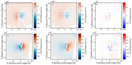
Figure 5.
Data displacement (a,d); Model Synthetic displacement (b,e); Residual displacement (c,f) of T012A and T121D, based on the optimal uniform slip model in Table 3.
4.3. Slip Distribution Inversion
In the second stage of inversion, we adopt the Steepest Descent Method (SDM) [5], developed by the German Research Centre for Geosciences, within a stratified crustal model to this study demonstrates the fault slip distribution. This approach formulates the inversion as a regularized least-squares problem. The objective function to be minimized is defined as the sum of the squared residuals between observed and modeled displacements plus a smoothing regularization term:
where represents the data misfit. is the vector of observed LOS displacements, is the Green’s function matrix, and x represents the slip distribution vector on subfaults. The second term is the smoothing constraint, where is a Laplacian operator and is the regularization parameter that balances the data misfit and the solution smoothness.
Compared to uniform slip models, distributed slip inversion provides a finer depiction of rupture complexity, though at the cost of increased parameter dimensionality. The geometric parameters and source location obtained from the prior non-linear inversion are used to constrain the linear inversion. The fault plane, with its overall strike and dip determined from our Bayesian inversion, is discretized into subfaults of 2 km × 2 km. To ensure a geophysically plausible solution, the rake angle for each subfault is then restricted to the range of −125° to −45°, a range informed by the focal mechanism solutions from multiple institutions (Table 1). LOS deformation observations are used as constraints to establish a linear mapping between surface displacements and fault slip components, enabling a detailed reconstruction of the fault’s internal kinematic structure. The inversion employs the CRUST1.0 Earth model (Table 4) [49], assuming a Poisson’s ratio of 0.25 for the elastic medium.
Table 4.
Crustal velocity model used for invention.
By comprehensively analyzing multiple datasets and incorporating field investigations from previous studies, this study identifies the DMCF as the seismogenic fault. The InSAR-derived deformation field clearly indicates that the rupture propagated to the surface, thus the upper boundary of the fault model is fixed at 0 km depth. To accommodate the full extent of the rupture zone, the fault plane is discretized with dimensions of 71 km along the strike and 30 km along the dip direction, based on the observed fault trace.
In order to ensure geophysically consistent and mechanically stable results, spatial smoothing constraints are incorporated into the inversion process, suppressing unrealistic slip variations and enhancing the robustness of the solution. The optimal smoothing parameter is selected through L-curve analysis, balancing data misfit and model roughness to achieve a reliable solution. The inversion is performed with a maximum of 10,000 iterations and a slip constraint of 10 m, yielding the final coseismic slip distribution (Figure 6).

Figure 6.
Slip distribution of the MS 6.8 Tingri earthquake: (a) Coseismic slip distribution on the seismogenic fault, with arrows indicating slip vectors; (b) Three-dimensional coseismic slip distribution model; (c) Surface projection of slip distribution, The red beach ball represents the focal mechanism solution from the GCMT project, and the cyan star is the surface projection of the centroid location derived from our slip distribution model (SDM) inversion. The red line indicates the surface trace of the DMCF, while the black lines denote other active faults in the region.
The slip distribution model indicates that the main rupture area of the 2025 Tingri earthquake extends roughly 38 km along strike and 25 km down-dip, with the majority of slip concentrated between depths of 1 and 15 km. Figure 6 highlights a distinct slip concentration near the surface of the ruptured fault plane, confirming that the coseismic rupture propagated to the surface. The maximum slip attains 5.36 m. The inversion estimates a moment magnitude (MW) of 7.12 for the 2025 Tingri earthquake, with the fault exhibiting a dip angle of 42.5°, an average rake of −114.94°, and a mean slip of 1.09 m. To evaluate the model’s reliability, the deformation field was simulated using the derived fault parameters (Figure 7), and residuals between observed and modeled displacements were calculated. As illustrated in the figure, the ascending track demonstrates good agreement with observations, showing only minor residuals. In contrast, the descending track exhibits a poorer fit on the eastern flank of the seismogenic fault. This discrepancy is mainly attributed to strong decorrelation effects in that region, which degrade the deformation signal and reduce measurement reliability. Furthermore, the presence of small-scale subsidiary faults with poorly constrained geometries introduces additional uncertainty to the inversion. Considering both the limited data quality and the absence of reliable fault parameter constraints, these secondary structures were excluded from the inversion to maintain the robustness of the fault model.

Figure 7.
Comparison between observed and modeled deformation fields for T012A and T121D tracks: (a,d) model coseismic deformation field; (b,e) simulated deformation field; (c,f) residuals.
5. Coulomb Stress Change Models
According to seismic cycle theory and Coulomb failure criterion, faults accumulate stress during inter-seismic periods until rupture [50], and the resulting Coulomb stress changes (≥0.1 bar) significantly modulate surrounding seismicity: increased stress promotes rupture while decreased stress inhibits it [51,52,53]. To evaluate the regional stress perturbations associated with the 2025 Tingri earthquake, we employed the PSGRN/PSCMP code [6], which computes coseismic Coulomb failure stress (CFS) changes based on a dislocation source embedded within a layered elastic half-space. The PSGRN/PSCMP code was used for this purpose, as it provides a robust elastic dislocation model while also offering the capability for future post-seismic viscoelastic modeling. The calculations were resolved onto receiver fault planes whose geometry was set to be consistent with our optimal inverted source fault model (strike 183°, dip 42.5°, rake −114.9°), as detailed in Table 5. This approach assesses the stress impact on optimally oriented faults within the study area. The calculations were performed for a depth range of 5–20 km, assuming an effective friction coefficient of 0.4 and a Poisson’s ratio of 0.25.
Table 5.
Geometric parameters of the receiver fault plane used for Coulomb stress change calculations.
The ΔCFS distribution patterns (Figure 8) exhibit pronounced spatial heterogeneity across four depth levels. Stress loading zones (ΔCFS > 0, red areas) predominantly align with the NE-SW orientation, particularly showing significant Coulomb stress increase (>0.03 MPa) near fault terminals and the DMCF periphery, thereby elevating seismic hazard in these regions. With increasing depth, the stress-enhanced zone progressively expands to the Nongqu Fault (NF), resulting in substantial stress accumulation. Conversely, NW-SE trending faults demonstrate stress release (ΔCFS < 0, blue areas), especially along the Shenzha–Dingjie Fault, Zada–Lazi–Qiongdojiang Fault system (ZLQF), and Dangreyongcuo–Xurucuo Fault, effectively reducing their seismic potential. These findings, consistent with recent tectonic studies of the DMCF [2,54], illuminate the control of deep-seated structures on coseismic stress redistribution and underscore the necessity for enhanced monitoring of high-ΔCFS zones.

Figure 8.
Coseismic Coulomb stress variations caused by the 2025 Tingri earthquake at multiple depths: (a) 5 km; (b) 10 km; (c) 15 km, and (d) 20 km. The red five-pointed star denotes the epicenter of the earthquake, and the black solid lines represent active faults.
In summary, the Tingri earthquake induced Coulomb stress changes demonstrate clear spatial heterogeneity and depth dependence. The elevated ΔCFS in the eastern STDS, southern Nongqu Fault, and southwestern DMCF indicates regions with a high potential for future seismic activity, underscoring the importance of focused seismic hazard assessment and continuous geophysical monitoring in these zones.
6. Discussion
6.1. Coherence Loss in Near-Field D-InSAR Observations
We observe severe coherence loss in the near-fault interferograms. Liu et al. [55] report that ~3 m surface ruptures in the graben created very large deformation gradients, causing Sentinel-1 C-band phase jumps exceeding half a wavelength. In practice, these steep fringes lead to unwrapping failures and interferogram gaps. To mitigate this, we masked low-coherence pixels (coherence < 0.4) as recommended by Yang et al. [54]. In general, interferometric coherence is easily destroyed by surface changes (vegetation, landslides, snow, etc.). In our case, the intense shaking, collapse of scatterers, and rapid ground deformation in the active graben largely explain the near-field decorrelation.
6.2. Fault Inversion Results and Deep Slip Phenomenon
Our initial modeling, which utilized a simplified single-dislocation source in a homogeneous elastic half-space (GBIS), yielded an optimal fault dip of ~42.5°. However, this single value derived from a simplified model may represent an “effective” or “averaged” dip rather than the true geometry for a distributed-slip inversion in a more realistic layered velocity structure. To address this critical point, we conducted an extensive grid search to systematically determine the optimal fault geometry. Our grid search systematically varied the dip at the top of the fault (Top_dip) from 50° to 89° and the dip at the bottom (Bottom_dip) from 5° to 45°. This search was replicated for four distinct modeling scenarios to assess the influence of data constraints (Sentinel-1 only vs. Sentinel-1 + LuTan-1) and structural complexity (single-fault vs. conjugate-fault models). The effort culminated in a comprehensive suite of 324 independent finite-fault inversions, with the detailed methodology and full results presented in Supporting Information Supplementary S2. This exhaustive search revealed a highly robust result: the data consistently favor a “listric” fault geometry with an extremely steep upper section (~89°) and a very shallow-dipping lower section (~5°). This finding of a near-surface, high-angle rupture is in excellent agreement with field observations from paleoseismic trenches by Tian et al. [56], who measured a near-surface fault dip of 73°. Our final preferred model utilizes this data-driven geometry.
Our finite-fault inversion suggests a west-dipping normal fault plane with a strike of approximately 183° (near N–S), a dip of ~42.5°, and a rake of ~−115°, indicating primarily dip-slip motion with a minor horizontal component. A similar fault geometry (strike ~189°, dip ~40°) was independently reported by Yu et al. [57], who also identified normal faulting as the dominant rupture mechanism. This interpretation is further supported by field observations, which reveal a surface rupture approximately 25–30 km in length, with vertical displacements reaching ~3 m and only limited lateral offset [58]. Thus, the slip vector is mostly downward on a dipping plane, with only a slight oblique component.
In addition, a minor amount of slip was detected at depths greater than ~20 km, potentially resulting from multiple contributing factors. First, based on the high-resolution relocated aftershock catalog obtained using the double-difference method by Yao et al. [59], it is evident that aftershocks persisted at depths below 20 km shortly after the mainshock (Figure 9). The presence of these deep aftershocks suggests that stress release in the lower crust may have been incomplete, potentially influencing the inversion results and yielding deep slip artifacts. Second, the selected fault plane geometry has a strong influence on the inversion outcome. In particular, when the selected rupture plane extends into a low-coherence region—such as the area on the eastern side—data quality deteriorates, reducing the reliability of constraints and possibly leading to spurious deep slip. Future research could integrate high-resolution spatiotemporal analysis of aftershock sequences, deep crustal imaging techniques (e.g., receiver function analysis and seismic tomography), and regional tectonic evolution modeling to better understand the physical mechanisms underlying the deep slip in this region, thereby improving the physical interpretability and reliability of finite-fault inversion results.

Figure 9.
Seismicity in the Dengmeduo graben region. A total of 31,038 early aftershocks were relocated using HypoDD (dots) [59]. Seismicity is concentrated along the Dengmocuo fault (the black solid lines are schematic fault traces). Five E–W cross-sectional profiles are plotted at 0.2° latitudinal intervals progressing from south to north across the study area. The color of each event dot denotes the corresponding aftershock occurrence time, as specified in the legend.
6.3. Improved Model Fit with a Conjugate Fault System and Analysis of Near-Field Residuals
To better constrain the near-field deformation, we incorporated the processed LT-1 dataset made publicly available by Qiao et al. [60]. The addition of this dataset allows us to investigate a key question: whether notable residuals in the near-field are caused by a suboptimal choice of the dip angle or if they point to more complex structural features. Our systematic grid search (as detailed in Supplementary S2) allows us to address this directly. We found that while optimizing the fault geometry (i.e., using the 89°/5° listric fault) does reduce residuals compared to a simple planar fault, the complexity of the fault structure itself, such as introducing a conjugate fault, plays an even more significant role in improving the data fit. Our tests confirm that a more complex, two-fault conjugate model significantly improves the fit to the geodetic data. As detailed in our analysis, incorporating a secondary conjugate fault structure, inspired by Qiao et al. [60], increased the data-model correlation from ~0.81 to ~0.89 and substantially reduced residuals (see Supplementary S1 Figures S2–S5 for a detailed comparison of all tested models). The slip was partitioned with the primary fault accommodating the vast majority of the moment release (~92%), indicating its dominance in the rupture process. This demonstrates that the conjugate geometry represents a more physically realistic depiction of the earthquake source.
While the conjugate model provides a scientifically refined solution, the single-fault model serves as an indispensable scientific benchmark within the scope of this study. This foundational approach is particularly pertinent given that our analysis is constrained to the publicly available Sentinel-1 dataset. Its primary role is twofold: it establishes a robust result using a standard methodology, providing a quantitative baseline against which more complex models can be rigorously evaluated; and it yields an excellent first-order approximation of the source. Our results show that the single-fault model successfully captures the fundamental source characteristics—including the faulting style, magnitude (MW ~7.1), and the location of peak slip. Therefore, the single-fault model is not presented as an alternative solution, but as a foundational component of our analytical progression, one that is essential for demonstrating the necessity and quantifying the improvement of the more refined conjugate fault system.
6.4. Comparison with Other Models: Similarities and Differences
Our results are broadly consistent with previous analyses of this event, particularly in terms of fault geometry and slip distribution, which are consistent with the findings of Yu et al. [57] and Xu et al. [58]: a ~20–30 km long normal fault trending N–S and dipping to the west, with peak coseismic slip of approximately 4–5 m. Xu et al. [58] mapped ~25–32 km of surface rupture with ~3 m vertical offset and only minor lateral offset, matching our modeled rupture length and displacement. However, a noteworthy discrepancy exists in the sense of the small strike-slip component. The results of Yu et al. [57] and Xu et al. [58] indicated a slight left-lateral motion, whereas our inversion yields a right-lateral component. This is a significant physical difference, not a matter of convention. As we will demonstrate in Section 6.4, the regional stress and strain fields provide a strong mechanical basis for favoring a right-lateral component of slip, allowing us to arbitrate between these competing kinematic models.
Conceptually, our findings better fit a distributed shear model than rigid block models. The event occurred in an interior extensional setting (the South Tibet Rift), not at a plate boundary. Unlike simple Andersonian normal-fault models (which would predict vertical σ1), the orientation here reflects a broader NNW–SSE σ1 and E–W σ3 regime. In fact, the fault lies on the southern (dextral) shear zone of the Lhasa block, in line with paired-shear deformation theories. In contrast to models of crustal extrusion or single-rift extension, the Tingri earthquake aligns with a system of conjugate shear faults under east–west extension. The event’s mechanism and orientation fall naturally out of a continuum shear framework rather than a rigid block translation model.
6.5. Seismogenic Mechanism and Regional Tectonics
The regional kinematic regime and tectonic setting provide a robust framework for interpreting our results. To establish this context, we first examine the crustal deformation pattern revealed by the GNSS-derived strain rate field from Pietrolungo et al. [61], focusing on our study area (Figure 10). This analysis reveals that the principal axis of horizontal contractional strain rate (εHmin) is oriented at ~341° (NNW) and the principal axis of horizontal extensional strain rate (εHmax) is at ~73° (ESE). This deformation is quantified by a dominant N–S contraction of [(20–30) × 10−9/year] across the ZLQF, accompanied by (~30 × 10−9/year) of E–W extension (Supplementary S1 Figure S1).

Figure 10.
Horizontal strain rate axes; Red and blue arrows denote the greatest extensional (εHmax) and contractional (εHmin) horizontal strain rates, respectively. The background color map illustrates the 2D dilatation strain rate, with blue indicating areal contraction and red representing dilatation. The red beach balls denote the GCMT focal mechanism solutions for this earthquake.
Complementing this kinematic picture, the regional stress field, derived independently from the inversion of earthquake focal mechanisms, illuminates the underlying dynamics. Pietrolungo et al. [61] demonstrate that in southern Tibet, the tectonic stress is characterized by a sub-horizontal, E-W to NW-SE oriented minimum principal stress axis (σ3), which is the driving force for extension. This stress orientation is consistent with the strain field and strongly supports a faulting mechanism characterized by extensional deformation [62]. The strain rate field also delineates a clear dilation–contraction transition zone bounded by the STDS, Shenzha–Dingjie Fault, Dangreyong Co Fault, and ZLQF, which marks the active tectonic boundary of the South Tibetan rift system [57].
Coulomb stress transfer modeling reveals that the earthquake increased Coulomb failure stress (ΔCFS ≥ 0.03 MPa) at both the northeastern and southwestern terminations of the rupture, predominantly along the fault strike. This suggests that adjacent north–south trending faults were brought closer to failure. Conversely, stress reductions occurred on major transverse fault systems, including east–west and oblique structures. As a result, the mainshock promoted failure on parallel normal-faulting systems while unloading stress on orthogonal faults. The distribution of aftershocks aligns closely with regions of increased ΔCFS, indicating effective stress transfer within the dextral shear zone of the Lhasa block. These patterns of stress redistribution and fault interaction further support an east–west extensional tectonic regime, which is consistent with the kinematic framework revealed by the geodetic strain data.
Furthermore, the established regional stress field serves as a powerful physical constraint to arbitrate between our coseismic slip model and previously published ones. As noted in Section 6.4, a key discrepancy is the sense of strike-slip motion; our model indicates a minor right-lateral component, whereas earlier studies suggested a left-lateral component. The tectonic setting is robustly defined by a persistent NNW-SSE compressional stress (maximum horizontal stress, SH_max) and ENE-WSW extension. When this stress field is resolved onto the ~N-S striking, west-dipping fault plane of the Tingri earthquake, it mechanically favors a right-lateral shear component in addition to the dominant normal slip. A left-lateral slip component, conversely, would be inconsistent with this well-established stress regime, requiring a significant and unobserved local rotation of the principal stress axes. This approach—using the background stress field to test the mechanical plausibility of competing features in coseismic slip models—is a powerful tool for model evaluation. For instance, Walbert and Hetland [63] successfully used this method to arbitrate between different slip models for the 2016 Kaikōura earthquake by assessing their consistency with the known slip history of nearby faults. Similarly, Szymanski et al. [64] demonstrated that a single-fault model for the 2020 Sparta earthquake was more mechanically plausible than a competing two-fault model because it better aligned with the regional stress field. Therefore, we argue that our right-lateral slip model is not only a valid fit to the geodetic data but is also more mechanically consistent with the regional tectonic environment.
6.6. Paired General-Shear (PGS) Deformation: Implications for Fault Evolution
Our finite-fault inversion reveals a west-dipping oblique-normal fault exhibiting a minor right-lateral slip component. Although the rupture is mainly extensional, this minor right-lateral motion aligns well with the regional stress and strain regime, making it kinematically plausible. In the Paired General-Shear (PGS) deformation proposed by Yin and Taylor [62], the Lhasa block lies within a southern right-lateral (dextral) shear zone, part of a broader east–west dual-shear system. This framework allows for local oblique faulting, where normal faults can be obliquely reactivated or newly formed under the influence of dextral shear. Our observed fault geometry—near N–S strike, west dip, and oblique-normal slip—is compatible with this tectonic setting.
We do not interpret the Tingri fault as a classic Riedel shear, nor do we suggest it is evolving into a strike-slip structure. Instead, the PGS model provides a kinematically plausible explanation for the slight dextral component observed in our inversion. It supports the interpretation that faulting in this segment of the South Tibet Rift occurs under oblique extension modulated by regional right-lateral shear.
The regional stress regime, primarily constrained by the inversion of earthquake focal mechanisms [61], shows a principal compressive axis (σ1) oriented at ~341° (NNW) and a principal extensional axis (σ3) at ~73° (ESE). This non-orthogonal stress orientation relative to the fault plane (strike ~183°, west-dipping) results in a resolved shear component on the fault surface.
Specifically, the ~20–30° angle between σ1 and the fault normal causes right-lateral shear stress on the fault, following the given relationship. This shear component explains the observed −115° rake, which incorporates a minor dextral offset. The oblique-normal slip is therefore a direct mechanical outcome of the regional stress field, rather than an anomalous feature.
The consistency between the fault’s slip vector and the oblique stress field lends further support to the application of the PGS model. In this context, the Tingri rupture represents a localized response to broader-scale right-lateral strain accommodation within the southern Lhasa block.
7. Conclusions
This study integrates Sentinel-1A radar data with the D-InSAR method to retrieve the coseismic deformation field of the 2025 MS 6.8 Tingri earthquake. The deformation field is masked out based on phase coherence, downsampled via the quadtree sampling technique, and inverted according to the elastic half-space dislocation theory model to examine fault slip. The coulomb stress alterations resulting from fault activity are computed, yielding the subsequent conclusions:
- The deformation field exhibits a butterfly shaped pattern (N-S ~160 km × E-W ~100 km), consistent with normal faulting. The ascending track shows maximum LOS displacements of +0.359 m and −0.841 m, while the descending track records +0.756 m and −1.09 m, respectively.
- Inversion identifies the seismogenic fault striking 183° (near N-S) with dip/slip angles of 42.5°/−114.94°. The maximum slip (5.36 m at shallow depth) yields a seismic moment of 3.32 × 10¹⁹ N·m (MW 7.12), confirming a normal-faulting event with surface rupture. The model achieves 81% fitting accuracy.
- The 2025 Tingri Mw 7.16 earthquake induced pronounced Coulomb stress perturbations across the Himalayan orogenic belt, characterized by distinct stress reduction along the eastern and western flanks of the DMCF, while triggering significant stress accumulation (ΔCFS > 0.1 bar) in several critical fault segments—notably the eastern STDS, southern Nongqu Fault, southwestern DMCF, and central Dajiling–Angren–Renbu Fault. Particularly intense stress loading was observed within the central rupture segment of the DMCF and its junction with the southern Nongqu Fault, where the combined effect of coseismic slip and geometric complexity generated localized stress concentrations exceeding 0.3 bar. These mechanically loaded fault segments now represent high-probability zones for future seismic activity, necessitating implementation of enhanced monitoring protocols including dense GNSS arrays, frequent InSAR acquisitions, and real-time seismic network optimization to better constrain the evolving seismic hazard potential.
- Based on our analysis, this study demonstrates that the coseismic rupture of this earthquake, characterized by its normal faulting mechanism and slip distribution, is a direct manifestation of the persistent N-S compressional and E-W extensional stress regime inherent to this tectonic domain.
Supplementary Materials
The following supporting information can be downloaded at: https://www.mdpi.com/article/10.3390/ijgi14110430/s1, Supplementary S1 Figure S1_S5.pdf and Supplementary S2 Systematic Grid Search for Optimal Fault Geometry of the Tingri Earthquake.pdf.
Author Contributions
Conceptualization, Zhen Wu and Huiwen Zhang; methodology, Zhen Wu and Zifei Ping; validation, Anan Chen; formal analysis, Anan Chen; investigation, Anan Chen; resources, Zhen Wu, Jianjian Wu and Jiayan Liao; data curation, Anan Chen; writing—original draft preparation, Anan Chen; writing—review and editing, Zhen Wu, Huiwen Zhang, Jianjian Wu, Zifei Ping and Jiayan Liao; visualization, Anan Chen; supervision, Zhen Wu; project administration, Zhen Wu; funding acquisition, Zhen Wu. All authors have read and agreed to the published version of the manuscript.
Funding
This study has been supported by six subjects, the Basic Scientific research Foundation of China Earthquake Administration (No. 2020IESLZ04); the Central Government Forest and Grassland Ecological Protection and Restoration Fund Project—Collection, Breeding, Cultivation, Reintroduction Technology, and Dynamic Monitoring of State Key Protected Wild Desert Plants in Gansu Province (No. KY202401); the Central Government Forest and Grassland Ecological Protection and Restoration Fund Project—Construction of Key and Endangered Wild Plant Conservation and Propagation Utilization Bases in Arid and Desert Areas (No. ZKY202306); the Project of Gansu Natural Science Foundation (No. 20JR5RA093); the Self-listed Program of Yunnan University (No. 2023KJF15); and the National Natural Science Foundation of China (No. 41761006).
Data Availability Statement
The raw data supporting the conclusions of this article will be made available by the authors on request.
Acknowledgments
The Sentinel-1 SAR (https://search.asf.alaska.edu/) data were provided by the ESA through their open data policy. The China Earthquake Networks Center and the National Earthquake Science Data Center (http://data.earthquake.cn, accessed on 27 January 2025) provided data support. Most Figures were plotted using Generic Mapping Tools (GMT). We used GBIS version 1.1 software. The SDM 2013 and PSGRN/PSCMP 2020 software were provided by Wang Rongjiang from the German Research Centre for Geosciences. We greatly appreciate the help provided by Bo Zhang, Junwen Zhu. The reviewers’ comments were very helpful in revising this paper, and we would like to express our gratitude to them as well.
Conflicts of Interest
The authors declare no conflicts of interest.
Abbreviations
The following abbreviations are used in this manuscript:
| SAR | Synthetic aperture radar |
| LOS | Line-of-sight |
| PGS | Paired general-shear |
| DMCF | Dengmecuo Fault |
| MFT | Main Frontal Thrust |
| MBT | Main Boundary Thrust |
| MCT | Main Central Thrust |
| STDS | Southern Tibetan Detachment System |
| YTSZ | Yarlung Tsangpo Suture Zone |
| GCMT | the Global Centroid Moment Tensor |
| USGS | the United States Geological Survey |
| CENC | the China Earthquake Networks Center |
| InSAR | Interferometric synthetic aperture radar |
| D-InSAR | Differential InSAR |
| COP-DEM | Copernicus Digital Elevation Model |
| GBIS | Geo-Bayesian Inversion Software |
| probability density function | |
| SDM | Steepest Descent Method |
| CFS | Coulomb failure stress |
| NF | Nongqu Fault |
| ZLQF | Zada–Lazi–Qiongdojiang Fault |
References
- Bai, L.; Chen, Z.; Wang, S. The 2025 Dingri MS6.8 Earthquake in Xizang: Analysis of Tectonic Background and Discussion of Source Characteristics. Rev. Geophys. Planet. Phys. 2025, 56, 258–263. [Google Scholar] [CrossRef]
- Shi, F.; Liang, M.; Luo, Q.; Qiao, J.; Zhang, D.; Wang, X.; Yi, W.; Zhang, J.; Zhang, Y.; Zhang, H.; et al. Seismogenic Fault and Coseismic Surface Deformation of the Dingri Ms 6.8 Earthquake in Tibet, China. Seismol. Geol. 2025, 47, 1–15. [Google Scholar] [CrossRef]
- Amey, R.M.J.; Hooper, A.; Walters, R.J. A Bayesian Method for Incorporating Self-Similarity into Earthquake Slip Inversions. J. Geophys. Res. Solid Earth 2018, 123, 6052–6071. [Google Scholar] [CrossRef]
- Bagnardi, M.; Hooper, A. Inversion of Surface Deformation Data for Rapid Estimates of Source Parameters and Uncertainties: A Bayesian Approach. Geochem. Geophys. Geosyst. 2018, 19, 2194–2211. [Google Scholar] [CrossRef]
- Wang, R.; Diao, F.; Hoechner, A. SDM—A Geodetic Inversion Code Incorporating with Layered Crust Structure and Curved Fault Geometry. In Proceedings of the EGU General Assembly Conference Abstracts, Vienna, Austria, 7–12 April 2013. [Google Scholar]
- Wang, R.; Lorenzo-Martín, F.; Roth, F. PSGRN/PSCMP—A New Code for Calculating Co- and Post-Seismic Deformation, Geoid and Gravity Changes Based on the Viscoelastic-Gravitational Dislocation Theory. Comput. Geosci. 2006, 32, 527–541. [Google Scholar] [CrossRef]
- Tapponnier, P.; Mercier, J.L.; Armijo, R.; Tonglin, H.; Ji, Z. Field Evidence for Active Normal Faulting in Tibet. Nature 1981, 294, 410–414. [Google Scholar] [CrossRef]
- Zhang, J.; Guo, L.; Ding, L. Structural Characteristics of the Central and Southern Segments of the Xainza-Dingjie Normal Fault System and Its Relationship with the Southern Tibet Detachment System. Chin. Sci. Bull. 2002, 47, 738–743. [Google Scholar] [CrossRef]
- Armijo, R.; Tapponnier, P.; Mercier, J.L.; Han, T.-L. Quaternary Extension in Southern Tibet: Field Observations and Tectonic Implications. J. Geophys. Res. Solid Earth 1986, 91, 13803–13872. [Google Scholar] [CrossRef]
- Zhao, B. Relocated Catalog of the M6.8 Tingri, Tibet Earthquake Sequence; National Earthquake Data Center: Golden, CO, USA, 2025. [CrossRef]
- Wu, X.; Xu, X.; Yu, G.; Ren, J.; Yang, X.; Chen, G.; Xu, C.; Du, K.; Huang, X.; Yang, H.; et al. The China Active Faults Database (CAFD) and Its Web System. Earth Syst. Sci. Data 2024, 16, 3391–3417. [Google Scholar] [CrossRef]
- Coleman, M.; Hodges, K. Evidence for Tibetan Plateau Uplift before 14 Myr Ago from a New Minimum Age for East–West Extension. Nature 1995, 374, 49–52. [Google Scholar] [CrossRef]
- Quidelleur, X.; Grove, M.; Lovera, O.M.; Harrison, T.M.; Yin, A.; Ryerson, F.J. Thermal Evolution and Slip History of the Renbu Zedong Thrust, Southeastern Tibet. J. Geophys. Res. Solid Earth 1997, 102, 2659–2679. [Google Scholar] [CrossRef]
- Ratschbacher, L.; Frisch, W.; Liu, G.; Chen, C. Distributed Deformation in Southern and Western Tibet during and after the India-Asia Collision. J. Geophys. Res. Solid Earth 1994, 99, 19917–19945. [Google Scholar] [CrossRef]
- Yin, A.; Harrison, T.M.; Murphy, M.A.; Grove, M.; Nie, S.; Ryerson, F.J.; Feng, W.X.; Le, C.Z. Tertiary Deformation History of Southeastern and Southwestern Tibet during the Indo-Asian Collision. GSA Bull. 1999, 111, 1644–1664. [Google Scholar] [CrossRef]
- Yin, A.; Harrison, T.M.; Ryerson, F.J.; Wenji, C.; Kidd, W.S.F.; Copeland, P. Tertiary Structural Evolution of the Gangdese Thrust System, Southeastern Tibet. J. Geophys. Res. Solid Earth 1994, 99, 18175–18201. [Google Scholar] [CrossRef]
- Bilham, R.; Gaur, V.K.; Molnar, P. Himalayan Seismic Hazard. Science 2001, 293, 1442–1444. [Google Scholar] [CrossRef]
- Avouac, J.-P.; Meng, L.; Wei, S.; Wang, T.; Ampuero, J.-P. Lower Edge of Locked Main Himalayan Thrust Unzipped by the 2015 Gorkha Earthquake. Nat. Geosci. 2015, 8, 708–711. [Google Scholar] [CrossRef]
- Houseman, G.; England, P. (Eds.) The Tectonic Evolution of Asia; World and Regional Geology Series; Cambridge University Press: Cambridge, UK, 1996; pp. 1–17. ISBN 978-0-521-48049-9. [Google Scholar]
- Wang, K.; Fialko, Y. Observations and Modeling of Coseismic and Postseismic Deformation Due to the 2015 Mw 7.8 Gorkha (Nepal) Earthquake. J. Geophys. Res. Solid Earth 2018, 123, 761–779. [Google Scholar] [CrossRef]
- McNamara, D.E.; Yeck, W.L.; Barnhart, W.D.; Schulte-Pelkum, V.; Bergman, E.; Adhikari, L.B.; Dixit, A.; Hough, S.E.; Benz, H.M.; Earle, P.S. Source Modeling of the 2015 Mw 7.8 Nepal (Gorkha) Earthquake Sequence: Implications for Geodynamics and Earthquake Hazards. Tectonophysics 2017, 714–715, 21–30. [Google Scholar] [CrossRef]
- Bai, L.; Klemperer, S.L.; Mori, J.; Karplus, M.S.; Ding, L.; Liu, H.; Li, G.; Song, B.; Dhakal, S. Lateral Variation of the Main Himalayan Thrust Controls the Rupture Length of the 2015 Gorkha Earthquake in Nepal. Sci. Adv. 2019, 5, eaav0723. [Google Scholar] [CrossRef]
- Chen, Y.; Li, W.; Yuan, X.; Badal, J.; Teng, J. Tearing of the Indian Lithospheric Slab beneath Southern Tibet Revealed by SKS-Wave Splitting Measurements. Earth Planet. Sci. Lett. 2015, 413, 13–24. [Google Scholar] [CrossRef]
- England, P.; Houseman, G. Extension during Continental Convergence, with Application to the Tibetan Plateau. J. Geophys. Res. Solid Earth 1989, 94, 17561–17579. [Google Scholar] [CrossRef]
- Lee, J.; Whitehouse, M.J. Onset of Mid-Crustal Extensional Flow in Southern Tibet: Evidence from U/Pb Zircon Ages. Geology 2007, 35, 45–48. [Google Scholar] [CrossRef]
- Li, J.; Song, X. Tearing of Indian Mantle Lithosphere from High-Resolution Seismic Images and Its Implications for Lithosphere Coupling in Southern Tibet. Proc. Natl. Acad. Sci. USA 2018, 115, 8296–8300. [Google Scholar] [CrossRef]
- Molnar, P.; Tapponnier, P. Active Tectonics of Tibet. J. Geophys. Res. 1978, 83, 5361–5375. [Google Scholar] [CrossRef]
- Pei, S.; Liu, H.; Bai, L.; Liu, Y.; Sun, Q. High-Resolution Seismic Tomography of the 2015 M7.8 Gorkha Earthquake, Nepal: Evidence for the Crustal Tearing of the Himalayan Rift. Geophys. Res. Lett. 2016, 43, 9045–9052. [Google Scholar] [CrossRef]
- Tian, X.; Chen, Y.; Tseng, T.-L.; Klemperer, S.L.; Thybo, H.; Liu, Z.; Xu, T.; Liang, X.; Bai, Z.; Zhang, X.; et al. Weakly Coupled Lithospheric Extension in Southern Tibet. Earth Planet. Sci. Lett. 2015, 430, 171–177. [Google Scholar] [CrossRef]
- Zhang, H.; Li, Y.E.; Zhao, D.; Zhao, J.; Liu, H. Formation of Rifts in Central Tibet: Insight from P Wave Radial Anisotropy. J. Geophys. Res. Solid Earth 2018, 123, 8827–8841. [Google Scholar] [CrossRef]
- Ryder, I.; Bürgmann, R.; Fielding, E. Static Stress Interactions in Extensional Earthquake Sequences: An Example from the South Lunggar Rift, Tibet. J. Geophys. Res. Solid Earth 2012, 117, 2012JB009365. [Google Scholar] [CrossRef]
- Aitchison, J.C.; Ali, J.R.; Davis, A.M. When and Where Did India and Asia Collide? J. Geophys. Res. Solid Earth 2007, 112, B05423. [Google Scholar] [CrossRef]
- Bettinelli, P.; Avouac, J.-P.; Flouzat, M.; Jouanne, F.; Bollinger, L.; Willis, P.; Chitrakar, G.R. Plate Motion of India and Interseismic Strain in the Nepal Himalaya from GPS and DORIS Measurements. J Geod. 2006, 80, 567–589. [Google Scholar] [CrossRef]
- Chen, Q.; Freymueller, J.T.; Wang, Q.; Yang, Z.; Xu, C.; Liu, J. A Deforming Block Model for the Present-Day Tectonics of Tibet. J. Geophys. Res. Solid Earth 2004, 109, B01403. [Google Scholar] [CrossRef]
- Wang, H.; Wright, T.J.; Liu-Zeng, J.; Peng, L. Strain Rate Distribution in South-Central Tibet from Two Decades of InSAR and GPS. Geophys. Res. Lett. 2019, 46, 5170–5179. [Google Scholar] [CrossRef]
- Wang, H.; Liu, M.; Cao, J.; Shen, X.; Zhang, G. Slip Rates and Seismic Moment Deficits on Major Active Faults in Mainland China. J. Geophys. Res. Solid Earth 2011, 116, B02405. [Google Scholar] [CrossRef]
- Xu, X. Late Quaternary Activity and Its Environmental Effects of the N-S Trend Kharta Fault in Xainza-Dinggye Rift, Southern Tibet. Master’s Thesis, China Earthquake Administration Institute of Geology, Beijing, China, 2019. [Google Scholar]
- He, P.; Wen, Y.; Ding, K.; Xu, C. Normal Faulting in the 2020 Mw 6.2 Yutian Event: Implications for Ongoing E–W Thinning in Northern Tibet. Remote Sens. 2020, 12, 3012. [Google Scholar] [CrossRef]
- Lasserre, C.; Peltzer, G.; Crampé, F.; Klinger, Y.; Van der Woerd, J.; Tapponnier, P. Coseismic Deformation of the 2001 M = 7.8 Kokoxili Earthquake in Tibet, Measured by Synthetic Aperture Radar Interferometry. J. Geophys. Res. Solid Earth 2005, 110, B12408. [Google Scholar] [CrossRef]
- Li, K.; Li, Y.; Tapponnier, P.; Xu, X.; Li, D.; He, Z. Joint InSAR and Field Constraints on Faulting during the Mw 6.4, July 23, 2020, Nima/Rongma Earthquake in Central Tibet. J. Geophys. Res. Solid Earth 2021, 126, e2021JB022212. [Google Scholar] [CrossRef]
- Wang, S.; Xu, C.; Wen, Y.; Yin, Z.; Jiang, G.; Fang, L. Slip Model for the 25 November 2016 Mw 6.6 Aketao Earthquake, Western China, Revealed by Sentinel-1 and ALOS-2 Observations. Remote Sens. 2017, 9, 325. [Google Scholar] [CrossRef]
- Fialko, Y.; Simons, M.; Agnew, D. The Complete (3-D) Surface Displacement Field in the Epicentral Area of the 1999 MW7.1 Hector Mine Earthquake, California, from Space Geodetic Observations. Geophys. Res. Lett. 2001, 28, 3063–3066. [Google Scholar] [CrossRef]
- Massonnet, D.; Rossi, M.; Carmona, C.; Adragna, F.; Peltzer, G.; Feigl, K.; Rabaute, T. The Displacement Field of the Landers Earthquake Mapped by Radar Interferometry. Nature 1993, 364, 138–142. [Google Scholar] [CrossRef]
- Qiu, J.; Ji, L.; Liu, L.; Liu, C. InSAR Coseismic Deformation and Tectonic Implications for the 2020 MW6.3 Nima Earthquake in Xizang. Seismol. Geol. 2021, 43, 1586–1599. [Google Scholar] [CrossRef]
- Okada, Y. Surface Deformation Due to Shear and Tensile Faults in a Half-Space. Bull. Seismol. Soc. Am. 1985, 75, 1135–1154. [Google Scholar] [CrossRef]
- Chen, T.; Akciz, S.O.; Hudnut, K.W.; Zhang, D.Z.; Stock, J.M. Fault-Slip Distribution of the 1999 Mw 7.1 Hector Mine Earthquake, California, Estimated from Postearthquake Airborne LiDAR Data. Bull. Seismol. Soc. Am. 2015, 105, 776–790. [Google Scholar] [CrossRef]
- Fukahata, Y.; Wright, T.J. A Non-Linear Geodetic Data Inversion Using ABIC for Slip Distribution on a Fault with an Unknown Dip Angle. Geophys. J. Int. 2008, 173, 353–364. [Google Scholar] [CrossRef]
- Jónsson, S.; Zebker, H.; Segall, P.; Amelung, F. Fault Slip Distribution of the 1999 Mw 7.1 Hector Mine, California, Earthquake, Estimated from Satellite Radar and GPS Measurements. Bull. Seismol. Soc. Am. 2002, 92, 1377–1389. [Google Scholar] [CrossRef]
- Laske, G.; Masters, G.; Ma, Z.; Pasyanos, M.E. CRUST1.0: An Updated Global Model of Earth’s Crust. Eur. Geosci. Union Gen. Assem. 2012, 14, 743. [Google Scholar]
- Milne, J. The California Earthquake of April 18, 1906. Nature 1910, 84, 165–166. [Google Scholar] [CrossRef]
- King, G.C.P.; Stein, R.S.; Lin, J. Static Stress Changes and the Triggering of Earthquakes. Bull. Seismol. Soc. Am. 1994, 84, 935–953. [Google Scholar] [CrossRef]
- Toda, S.; Stein, R.S.; Richards-Dinger, K.; Bozkurt, S.B. Forecasting the Evolution of Seismicity in Southern California: Animations Built on Earthquake Stress Transfer. J. Geophys. Res. Solid Earth 2005, 110, B05S16. [Google Scholar] [CrossRef]
- Shi, Y.; Cao, J. Some Aspects in Static Stress Change Calculation—Case Study on Wenchuan Earthquake. Chin. J. Geophys. 2010, 53, 102–110. [Google Scholar] [CrossRef]
- Yang, J.; Jin, M.; Ye, B.; Li, Z.; Li, Q. Source Rupture Mechanism and Stress Changes to the Adjacent Area of January 7, 2025, MS 6.8 Dingri Earthquak. Seismol. Geol. 2025, 47, 36. [Google Scholar] [CrossRef]
- Liu, Q.; Hua, J.; Zhang, Y.; Gong, W.; Zang, J.; Zhang, G.; Li, H. Geodetic Observations and Seismogenic Structures of the 2025 Mw 7.0 Dingri Earthquake: The Largest Normal Faulting Event in the Southern Tibet Rift. Remote Sens. 2025, 17, 1096. [Google Scholar] [CrossRef]
- Tian, T.; Wu, Z. Recent Prehistoric Major Earthquake Event of Dingmucuo Normal Fault in the Southern Segment of Shenzha-Dingjie Rift and Its Seismic Geological Significance. Geol. Rev. 2023, 69, 53–55. [Google Scholar] [CrossRef]
- Yu, S.; Zhang, S.; Luo, J.; Li, Z.; Ding, J. The Tectonic Significance of the Mw7.1 Earthquake Source Model in Tibet in 2025 Constrained by InSAR Data. Remote Sens. 2025, 17, 936. [Google Scholar] [CrossRef]
- Xu, X.; Wang, S.; Cheng, J.; Wu, X. Shaking the Tibetan Plateau: Insights from the Mw 7.1 Dingri Earthquake and Its Implications for Active Fault Mapping and Disaster Mitigation. npj Nat. Hazards 2025, 2, 16. [Google Scholar] [CrossRef]
- Yao, J.; Yao, D.; Chen, F.; Zhi, M.; Sun, L.; Wang, D. A Preliminary Catalog of Early Aftershocks Following the 7 January 2025 MS6.8 Dingri, Xizang Earthquake. J. Earth Sci. 2025, 36, 856–860. [Google Scholar] [CrossRef]
- Qiao, X.; Lu, Z.; Yan, S.; Shi, H.; Zhi, M.; Zhao, D. The 2025 MW7.0 Dingri Earthquake: Conjugate Normal Faulting of a Graben Structure in the Southern Xainza-Dinggye Rift. Geophys. Res. Lett. 2025, 52, e2025GL116154. [Google Scholar] [CrossRef]
- Pietrolungo, F.; Lavecchia, G.; Madarieta-Txurruka, A.; Sparacino, F.; Srivastava, E.; Cirillo, D.; de Nardis, R.; Andrenacci, C.; Bello, S.; Parrino, N.; et al. Comparison of Crustal Stress and Strain Fields in the Himalaya–Tibet Region: Geodynamic Implications. Remote Sens. 2024, 16, 4765. [Google Scholar] [CrossRef]
- Yin, A.; Taylor, M.H. Mechanics of V-Shaped Conjugate Strike-Slip Faults and the Corresponding Continuum Mode of Continental Deformation. GSA Bull. 2011, 123, 1798–1821. [Google Scholar] [CrossRef]
- Walbert, O.L.; Hetland, E.A. Bayesian Inference of Seismogenic Stress for the 2016 Mw 7.8 Kaikōura, New Zealand, Earthquake. Bull. Seismol. Soc. Am. 2022, 112, 1894–1907. [Google Scholar] [CrossRef]
- Szymanski, E.D.; Hetland, E.A.; Figueiredo, P.M. Imaging Left-lateral and Reverse Near-surface Slip of the 2020 Mw 5.1 Sparta, North Carolina, Earthquake. Bull. Seismol. Soc. Am. 2024, 114, 1870–1883. [Google Scholar] [CrossRef]
Disclaimer/Publisher’s Note: The statements, opinions and data contained in all publications are solely those of the individual author(s) and contributor(s) and not of MDPI and/or the editor(s). MDPI and/or the editor(s) disclaim responsibility for any injury to people or property resulting from any ideas, methods, instructions or products referred to in the content. |
© 2025 by the authors. Published by MDPI on behalf of the International Society for Photogrammetry and Remote Sensing. Licensee MDPI, Basel, Switzerland. This article is an open access article distributed under the terms and conditions of the Creative Commons Attribution (CC BY) license (https://creativecommons.org/licenses/by/4.0/).