Article

Using Certainty Factor as a Spatial Sample Filter for Landslide Susceptibility Mapping: The Case of the Upper Jinsha River Region, Southeastern Tibetan Plateau

1
Key Laboratory of Hydraulic and Waterway Engineering, Ministry of Education, Chongqing Jiaotong University, Chongqing 400074, China
2
College of Geological and Surveying Engineering, Taiyuan University of Technology, Taiyuan 030024, China
3
College of Construction Engineering, Jinlin University, Changchun 130012, China
4
College of Transportation and Civil Engineering, Fujian Agriculture and Forestry University, Fuzhou 350002, China
5
Key Laboratory of Mountain Hazards and Earth Surface Process, Institute of Mountain Hazards and Environment, Chinese Academy of Sciences, Chengdu 610041, China
*
Author to whom correspondence should be addressed.
ISPRS Int. J. Geo-Inf. 2025, 14(9), 339; https://doi.org/10.3390/ijgi14090339
Submission received: 7 July 2025 / Revised: 26 August 2025 / Accepted: 29 August 2025 / Published: 1 September 2025

Abstract

Landslide susceptibility mapping (LSM) faces persistent challenges in defining representative stable samples as conventional random selection often includes unstable areas, introducing spatial bias and compromising model accuracy. To address this, we redefine the certainty factor (CF) method—traditionally for factor weighting—as a spatial screening tool for stable zone delineation and apply it to the tectonically active upper Jinsha River (937 km2, southeastern Tibetan Plateau). Our approach first generates a preliminary susceptibility map via CF, using the natural breaks method to define low- and very low-susceptibility zones (CF < 0.1) as statistically stable regions. Non-landslide samples are exclusively selected from these zones for support vector machine (SVM) modeling with five-fold cross-validation. Key results: CF-guided sampling achieves training/testing AUC of 0.924/0.920, surpassing random sampling (0.882/0.878) by 4.8% and reducing ROC standard deviation by 32%. The final map shows 88.49% of known landslides concentrated in 25.70% of high/very high-susceptibility areas, aligning with geological controls (e.g., 92% of high-susceptibility units in soft lithologies within 500 m of faults). Despite using a simpler SVM, our framework outperforms advanced models (ANN: AUC, 0.890; RF: AUC, 0.870) in the same region, proving physical heuristic sample curation supersedes algorithmic complexity. This transferable framework embeds geological prior knowledge into machine learning, offering high-precision risk zoning for disaster mitigation in data-scarce mountainous regions.

1. Introduction

Landslides are among the most devastating natural hazards in mountainous areas across the globe. The upper reaches of the Jinsha River, located on the southeastern edge of the Tibetan Plateau, are marked by intricate terrain and vigorous tectonic uplift. Here, landslides exert grave dangers on both infrastructure and local communities. Landslide susceptibility mapping (LSM) is frequently deemed a crucial preliminary step for landslide risk evaluation and serves as a key instrument underpinning decision-making processes. Identifying landslide-prone areas and creating susceptibility maps are crucial for early warning systems against landslide disasters. Utilizing the results of susceptibility evaluations can reduce substantial losses, such as damage to buildings, casualties, and property loss [1]. These landslide susceptibility maps can directly provide references for land use and planning. However, their accuracy is challenged by multiple factors, including the critical but understudied issue of non-landslide sample selection [2,3,4,5].
Landslide susceptibility mapping includes processes such as the development of a landslide inventory, the division of evaluation units, the selection of influencing factors, and the modeling of susceptibility evaluations. To obtain accurate predictive models, scholars have proposed and applied various methods to enhance the precision of model predictions. For example, Pourghasemi and Rossi (2017) [6] reviewed 220 studies related to landslide susceptibility evaluation and summarized up to 41 landslide influencing factors. However, it is usually impractical to consider all these factors in susceptibility evaluations. Instead, the most relevant factors are selected based on the actual situation of the landslides for overlay analysis. Some scholars have suggested using techniques such as correlation coefficient analysis [7,8], principal component analysis [8], and information gain ratio [9] to filter influencing factors, followed by applying machine learning techniques such as logistic regression models [10], discriminant analysis models [11], fuzzy logic models [12], artificial neural network models [13], support vector machine models (SVM) [14], decision tree models [15], and neuro-fuzzy models [16] for landslide susceptibility mapping. Later, some scholars found that machine learning techniques used for LSM have inherent uncertainty and suggested using ensemble learning methods that combine multiple machine learning techniques to quantify this uncertainty, believing that ensemble models have better classification effects on landslides than single machine learning technique models [17]. While factor optimization and algorithm selection have been thoroughly investigated [4,18,19], the selection strategy for non-landslide samples—traditionally relying on random sampling with distance constraints (e.g., ≥200 m from known landslides)—introduces inherent spatial bias [1,20]. Recent studies confirm that such approaches risk including de facto unstable areas within “stable” samples, significantly compromising model reliability [2,21]; for example, Ozturk et al. (2021) [2] systematically explored the impact of landslide sample size, location, and temporal factors on landslide susceptibility evaluation results, suggesting that sampling the lower sedimentary cover area of landslides (without sampling the entire landslide) can lead to better model performance, and medium-sized landslides (104~106 m2) can result in better model effects when sampled for landslides, while spatially or temporally stratified sampling has only a small impact on model performance. However, the current selection of non-landslide data mostly adopts the method of random generation in the study area, and some non-landslide data may fall into the high-landslide-susceptibility area, resulting in the decline of model prediction accuracy. This fundamental gap in defining true stable zones limits practical applications of LSM, particularly in geologically complex terrains like our study area. Therefore, it is very important to seek a reasonable collection method of non-landslide data [22,23].
To address this limitation, we propose a paradigm shift in non-landslide sampling. Instead of treating the certainty factor (CF) method solely as a factor-weighting tool [24], we innovatively repurpose it as a spatial screening mechanism to delineate statistically stable zones for sample selection. First, based on the complex geological environment conditions in the upper reaches of the Jinsha River, a landslide susceptibility evaluation index system applicable to this area is established. Then, the slope units are divided based on the curvature watershed method. Next, CF is applied to generate a preliminary susceptibility map identifying low/very low-susceptibility areas as proxies for true stable regions. Then, non-landslide units are randomly sampled exclusively from these zones. Finally, both landslide and screened non-landslide samples are inputted into an SVM model. This framework (CF mapping + SVM classification) fundamentally redefines the role of heuristic methods in data-driven LSM. While prior studies combined CF with SVM for factor integration [25], our aim is to leverage CF explicitly for spatial sample purification, effectively embedding geological prior knowledge into the training data structure. The research in this study can be used to compare CF-guided sampling with conventional random sampling, and to determine whether sample screening based on physical heuristics is superior to pure algorithmic enhancement (for example, artificial neural network [26,27] or random forest [28,29]). These research results can be used to deliver a transferable LSM framework for similar mountainous regions.

2. Study Area

The research zone (99.157–99.245° E, 28.739–28.217° N) lies along the main course of the Jinsha River, straddling the border between the Sichuan and Yunnan provinces, with the river itself forming the dividing line (Figure 1). As part of the upper reaches of the Jinsha River, this area features a terrain that slopes downward from south to north, accompanied by swift currents. The flanking mountains rise steeply while the valleys run deep, forming a distinct “V”-shaped landform [1,30,31]. The total length of the study reach is about 937 km2, flowing through several villages. There are many faults in the area, most of which are trending north–south. In the past, earthquake activities were mainly limited to small earthquakes, and no destructive earthquakes with high magnitude have occurred. Due to the constraints and influences of plate tectonics and fault structures, the topography and landforms in the area are complex, with extensive distribution of high mountain canyons, and most areas are located at an altitude of 2200–4200 m. The climate and vegetation distribution show vertical zonation characteristics, with relatively low rainfall, which roughly increases linearly with altitude. The stratigraphic lithology is complex, with the main strata being the Mesoproterozoic Xiongsong Group (Pt2X) and the Paleozoic Jinshajiang Ophiolite Group (DTJ).

3. Materials and Methods

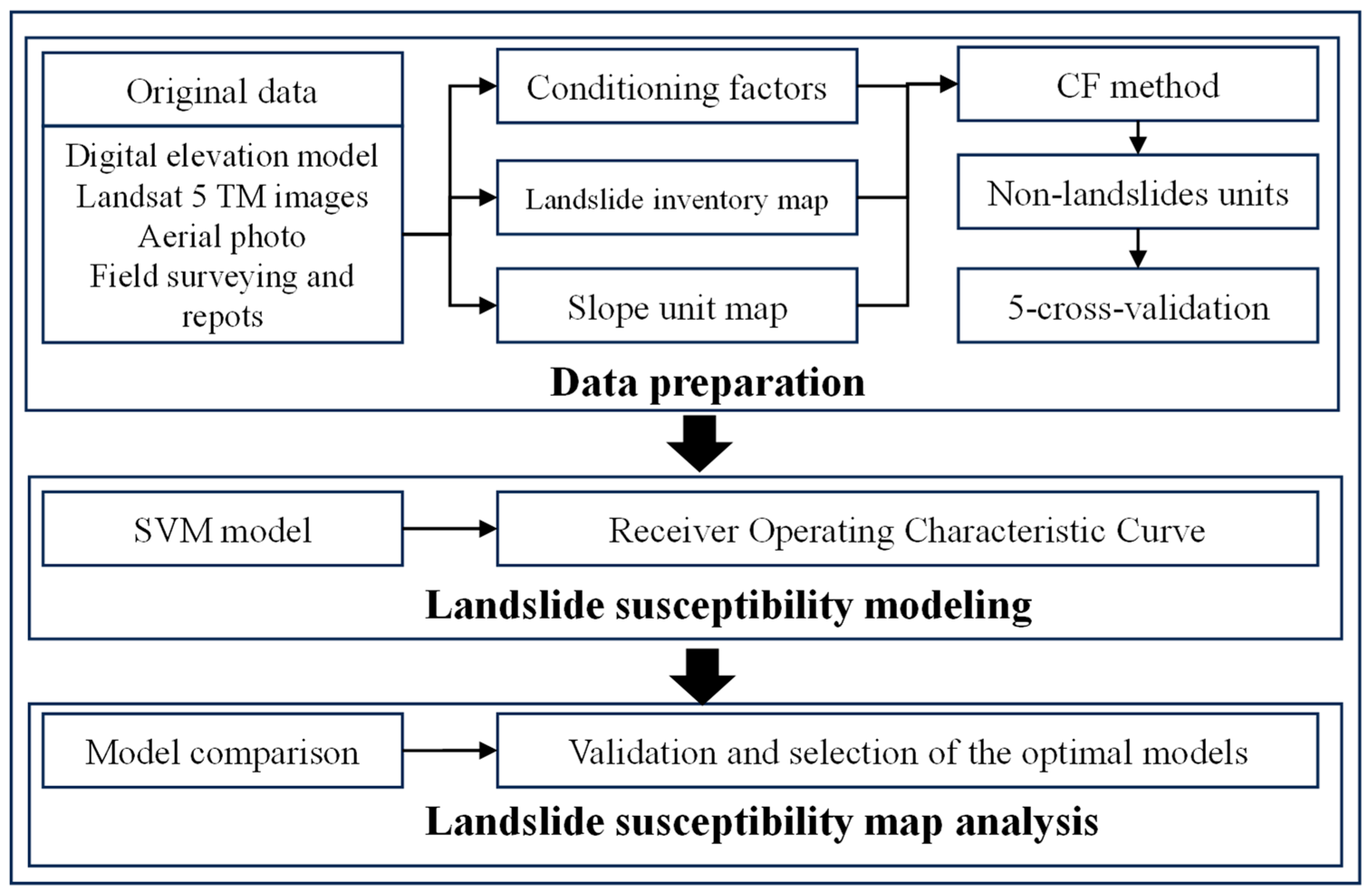
Figure 2 shows the three main steps of this study, including (a) data preparation, (b) landslide susceptibility modelling, (c) landslide susceptibility map analysis.

3.1. Landslide Inventory

The landslide inventory is derived from remote sensing interpretation and landslide surveys. By leveraging the features of landslides on remote sensing images and three-dimensionally integrating information such as actual terrain, structural characteristics, and river erosion, a more lifelike depiction of the site can be obtained. This offers a simple, accurate, and rapid approach to landslide interpretation. With the assistance of ArcGIS software, a three-dimensional comprehensive remote sensing interpretation map was finally created, which effectively facilitates landslide interpretation [1,30,31]. By using the high-resolution three-GNSS image (5 m) and the digital elevation model (5 m) to establish a three-dimensional model of the study area, the existing landslides were identified. Potential landslides were interpreted from the Sentinel-1 data, and the interpretation results were verified and supplemented through on-site investigations. A total of 61 landslides were identified in the study area. (Figure 1a). The types of these unstable slopes include glacial till, landslide deposits, and unstable deposits (Figure 3).

3.2. Mapping Units

As the core unit in landslide susceptibility mapping, the mapping unit plays a pivotal role in shaping research findings. Presently, diverse mapping units are used for surface segmentation, falling mainly into five types [1]: (a) watershed unit; (b) slope unit; (c) grid unit; (d) uniform condition unit; and (e) regional unit [19]. Of these frequently used units, the grid unit is the most widespread [32]. However, its loose connection with terrain and other geological data has led to a growing focus on the slope unit, defined by topographic traits, among relevant academics. It is widely recognized that within a given area, the slope unit is bounded by watershed lines and catchment lines, potentially covering multiple slopes or even an entire small watershed, making it better suited for landslide susceptibility mapping studies [33]. Through a summary of domestic and international slope unit division methodologies, four commonly applied methods are identified: (a) the r.slopeunits method; (b) the curvature watershed method; (c) the MIA-HUS method; (d) the hydrological analysis method. Sun et al. [1] compared the results of the hydrological analysis method and the curvature watershed method, noting that the latter divides the entire area into slope units based on changes in slope and aspect. This approach not only identifies watershed and catchment lines but also differentiates between horizontal and inclined surface boundaries. The divided units feature uniform areas, with fewer irrational ones, and the division results are more reasonable. Consequently, this paper adopts the curvature watershed method for the division of mapping units, and the basic flow chart is presented in Figure 4 [1].

3.3. Conditioning Factors

For constructing a rational index system for landslide susceptibility assessment, the selection of evaluation indicators must be rooted in a comprehensive comprehension of the landslide traits within the study area, integrating a literature review, field surveys, and regional geological settings. The study area, located on the southeastern fringe of the Tibetan Plateau, is characterized by intense tectonic activity, high topographic relief, and a vertical climate, i.e., vegetation zonation. We first reviewed many representative LSM studies in the Jinsha River basin and Tibetan Plateau [15,34,35,36,37] to identify commonly used factors then validated and supplemented these through three field surveys (2021–2022) covering the entire 130 km study reach. Surveys confirmed that local landslides are primarily controlled by lithology (soft rock fragmentation), fault activity (rock mass disturbance), river erosion (slope undercutting), and vegetation cover (root reinforcement). Combining these insights with data availability (e.g., rainfall data from local meteorological stations and NDVI from Sentinel-2 imagery), 14 conditioning factors were finally selected to form the evaluation index system [20,38]. These factors are as follows: (1) lithological factors, including (a) lithology and (b) rock hardness; (2) topographic factors, including (c) elevation, (d) slope angle, (e) slope aspect, (f) topographic relief, and (g) curvature; (3) vegetation factors, including (h) land use and (i) normalized difference vegetation index (NDVI); (4) geological structural factors, including (j) distance from faults; (5) terrain uplift factors, including (k) Strahler’s integral value; (6) river factors, including (l) distance from rivers; (7) rainfall, including (m) rainfall; and (8) seismic factors, including (n) earthquake intensity. The index system is illustrated in Figure 5. The data sources of each conditioning factor extraction and the mutator methods of each conditioning factor to the slope unit are listed in Table 1.

3.4. Multicollinearity Analysis of Conditioning Factors

Collinearity among conditioning factors may undermine assessment results [32], thus requiring thorough elimination. Principal component analysis (PCA), a technique for reducing dimensionality, functions fundamentally by transforming original variables into a fresh set of uncorrelated principal components. It prioritizes components that capture the greatest share of variance in the dataset: the first component takes up the largest variance, the second accounts for the remaining variance while staying orthogonal to the first, and this sequence proceeds [40,41,42]. By retaining components with the largest eigenvalues (which signify their contribution to variance), PCA maps high-dimensional data onto a lower-dimensional subspace, achieving a balance between information retention and dimensionality reduction. This process effectively sifts out noise and redundancy, emerging as a vital tool for simplifying complex datasets while preserving crucial patterns. Hence, PCA is adopted to remove multicollinearity among the conditioning factors.

3.5. Sampling Method for Non-Landslide Points

Recent LSM studies have developed rigorous non-landslide selection methods to avoid false stable samples, which are mainly categorized into three types.
Spatial constraint-based methods: Ozturk et al. (2021) [2] used multi-distance buffer stratification (200–500 m, 500–1000 m from landslides) and lithological zoning to reduce clustering, while Rossi et al. (2010) [33] sampled from homogeneous topographic units (e.g., slope units). However, fixed buffers (e.g., 200 m) are geologically arbitrary, and unit-based sampling relies on complete historical inventories, which are scarce in the upper Jinsha River.
Heuristic/knowledge-driven methods: Chen et al. (2016) [43] and Cao et al. (2016) [34] used CF/FR to identify low-susceptibility factor subclasses (e.g., hard lithologies) but only for factor weighting, not spatial sampling. Kumar et al. (2023) [35] excluded fault/erosion zones but needed detailed geological maps unavailable here.
Data-driven methods: Dey et al. (2024) [42] used K-means clustering, and Wang et al. (2022) [5] used pre-trained RF models. These require large datasets (thousands of samples), which are impractical for our study (only 61 unstable slopes).
In the process of building a landslide susceptibility mapping model, non-landslide units in quantities matching those of landslide units are required for model construction. A key drawback of the conventional random sampling approach for non-landslide units lies in its possible inclusion of unstable zones within “stable” samples, thereby introducing spatial bias [2]. To overcome this, we propose a novel two-stage framework that redefines the role of heuristic methods:
(a) Physically guided stable zone delineation using certainty factor (CF)
The CF method, conventionally applied for factor weighting [25,44,45,46], is innovatively repurposed as a spatial screening tool. We compute CF values for each conditioning factor subclass using Equation (1):
C F = P P a P P s P P a ( 1 P P s )           P P a P P s P P a P P s P P s ( 1 P P a )           P P a < P P s
where PPa is the ratio of the number of occurrences of a certain event in a subclass of evaluation indicators to the total number of samples in that subclass; and PPs is the ratio of the total number of event occurrences to the total number of samples. From the definition and calculation process of the CF value, it can be seen that the CF value is a number within the range of [−1, 1]. When the CF value is greater than 0, this indicates that the event is highly sensitive to a certain factor, and this factor is conducive to the occurrence of the event. The closer the CF value is to 1, the higher the sensitivity of this factor. However, when the CF value is less than 0, the opposite is true. This indicates that the event is less sensitive to a certain factor, and this factor is not conducive to the occurrence of the event. The closer the CF value is to −1, the lower the sensitivity of this factor.
This generates a preliminary susceptibility map where low/very low-susceptibility zones (statistically stable areas) are identified as candidate regions for non-landslide sampling.
(b) Spatial-constrained sampling
Non-landslide units are selected exclusively from these stable zones, contrasting sharply with conventional random sampling (a ≥200 m buffer, making sure to prevent the influence of existing landslides on non-landslide data).
To isolate the impact of sampling strategies, all models share identical slope units, identical PCA-reduced factors are used, and identical five-fold cross-validation partitions are applied. This rigorous design ensures that any accuracy improvement is directly attributable to our CF-guided sampling framework.
By using this method, the following breakthroughs are made: (a) it transforms CF from a factor evaluator to a sample filter—a paradigm shifts beyond prior CF-SVM integrations [25]; and (b) it embeds geological prior knowledge into data preparation, reducing machine learning’s “black-box” uncertainty [17].

3.6. Landslide Susceptibility Mapping Model

The support vector machine (SVM) has become a robust tool in landslide susceptibility zoning thanks to its strong ability to manage complex nonlinear relationships and high-dimensional data. As a supervised machine learning algorithm, SVM creates optimal hyperplanes to maximize the margin between different classes, which makes it especially suitable for distinguishing between landslide-prone areas and stable regions [43,47]. In analyzing landslide susceptibility, the support vector machine (SVM) proves effective at integrating a range of influencing factors—like topography, rock type, precipitation, and human-induced activities—to model the nonlinear relationships that trigger landslides. Its kernel function, such as the radial basis function (RBF), allows for the flexible conversion of input data into higher-dimensional feature realms, enhancing the model’s ability to detect intricate patterns [14,48]. When contrasted with conventional statistical approaches, SVM stands out for its strengths in preventing overfitting, managing limited sample sizes, and sustaining high predictive precision. This explains its widespread use in mapping regional landslide susceptibility.

3.7. Validation Methods

3.7.1. K-Fold Cross-Validation

In landslide susceptibility mapping, the application of k-fold cross-validation entails dividing spatial datasets into k mutually exclusive subsets. During each iteration, k-1 subsets act as the training set for calibrating predictive models, and the remaining one is utilized for validation. This procedure is repeated k times, with each data point being validated exactly once [1,30]. Particularly in landslide research, this method reduces spatial bias and overfitting by systematically assessing the model’s generalizability across various geographic segments.

3.7.2. Receiver Operating Characteristic (ROC) Curve

The receiver operating characteristic (ROC) curve offers a visual means to evaluate binary classification models. It does this by graphing the true positive rate (TPR) against the false positive rate (FPR) across a range of threshold values. TPR (sensitivity) measures correctly identified actual positives; FPR (related to 1-specificity) reflects actual negatives misclassified as positive [49,50,51]. The curve shape and area under the curve (AUC) indicate classification ability: AUC = 1 for perfect performance and 0.5 for random. In landslide susceptibility mapping, ROC curves help compare models and balance correct detections with false alarms.

4. Results

4.1. Result of Slope Unit Division and Non-Landslide Units Sampling

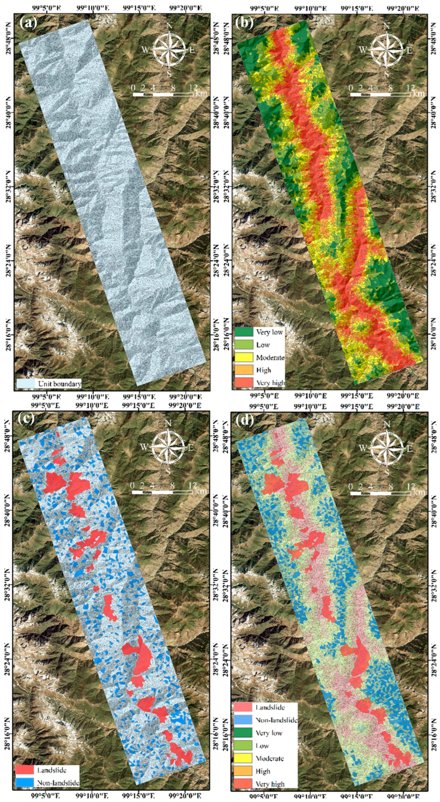
Grid resolution has a major bearing on the size of the slope units divided using the curvature watershed approach. In this research, multiple thresholds were tested through trial computations to compare how slope units turned out under different settings. These results were then pitted against high-precision Resource-3 image data to refine the division quality. For splitting slope units, the DEM data resolution was adjusted to 5.0 m × 5.0 m, 10.0 m × 10.0 m, 30.0 m × 30.0 m, 50.0 m× 50.0 m, 80.0 m× 80.0 m, 100.0 m× 100.0 m, and 120.0 m× 120.0 m. Findings show that the best division emerged at a DEM resolution of 100.0 m× 100.0 m, with 5421 units in total, of which the most significant unit is 1.048 km2, and the smallest unit is 0.001 km2 (Figure 6a).
Using the study area’s landslide inventory and slope unit division outcomes, 575 units with landslides were pinpointed. First, an equal number of non-landslide units were picked at random from zones at least 200 m away from the landslide units, serving as the first batch of non-landslide samples (Figure 6c). Second, drawing on the study area’s landslide susceptibility map (Figure 6b) computed via the CF value (Figure 7), non-landslide units—matching the count of landslide units—were selected randomly from its low/very low-susceptibility areas (the threshold was determined via the natural breaks (Jenks) method) to form the second group of non-landslide samples (Figure 7d).
According to the certainty factor (CF) calculation results, the stratigraphic lithologies that are most likely to trigger landslides, ranked from high to low, are Ψo (0.58), Pgj (0.37), DTJ (0.25), and D2q (0.18). As rock mass hardness increases, the CF value decreases gradually, meaning that soft and relatively soft rocks are more prone to landslides. In terms of elevation distribution, the elevation range of 2000–2800 m has the highest CF value, indicating that this range provides the most favorable conditions for landslides to occur. The slope intervals that are most conducive to landslides are 4–26° and 29–32°, and slopes facing southwest and west have higher susceptibility. Areas with a relief amplitude greater than 1000 m are more likely to experience landslides, and convex slopes are more vulnerable than slopes of other shapes. The CF value generally decreases as the distance from faults increases, which suggests that faults have a certain control over landslides in the study area. The closer a location is to faults, the more fragmented the rock mass structure, making it easier for landslides to happen. The Strahler integral value that is most favorable for landslides is below 0.44, which corresponds to the geomorphic development stage from late mature to old age. At this stage, the exogenic forces (such as weathering and erosion) acting on slope units are stronger than the endogenic forces (such as tectonic activities), which promotes the occurrence of landslides. Bare land is more sensitive to landslides because it lacks vegetation protection, leading to intensified erosion by surface water, a higher degree of weathering, fragmented rock mass, and reduced slope stability. The NDVI (Normalized Difference Vegetation Index) range of −0.02 to 0.17, which largely overlaps with bare land areas, is conducive to the occurrence of landslides. The CF value generally decreases as the distance from rivers increases, mainly because being closer to rivers enhances fluvial down-cutting erosion, resulting in steeper slopes along riverbanks. Slope instability along rivers often leads to landslides as a way to adapt to erosional forces. In addition, slope bodies near rivers are soaked by river water at their feet, which reduces the strength of rock and soil masses and promotes landslides. Most landslides in the study area occur in regions with low annual rainfall, which is attributed to the dry-hot valley climate and high-altitude (above 4800 m) snowfall, which rarely form sufficient rainfall to trigger landslides over a short period. It is worth noting that the impact of seismic intensity on landslides does not show a clear increasing trend with higher intensity, lacking obvious regularity. This is because most landslides in the study area were not induced by the current earthquake, weakening the correlation between seismic intensity and landslide distribution. However, seismic intensity still shows a certain correlation, and as a key triggering factor, earthquakes should be given priority in landslide susceptibility analysis.

4.2. Multicollinearity Analysis Results

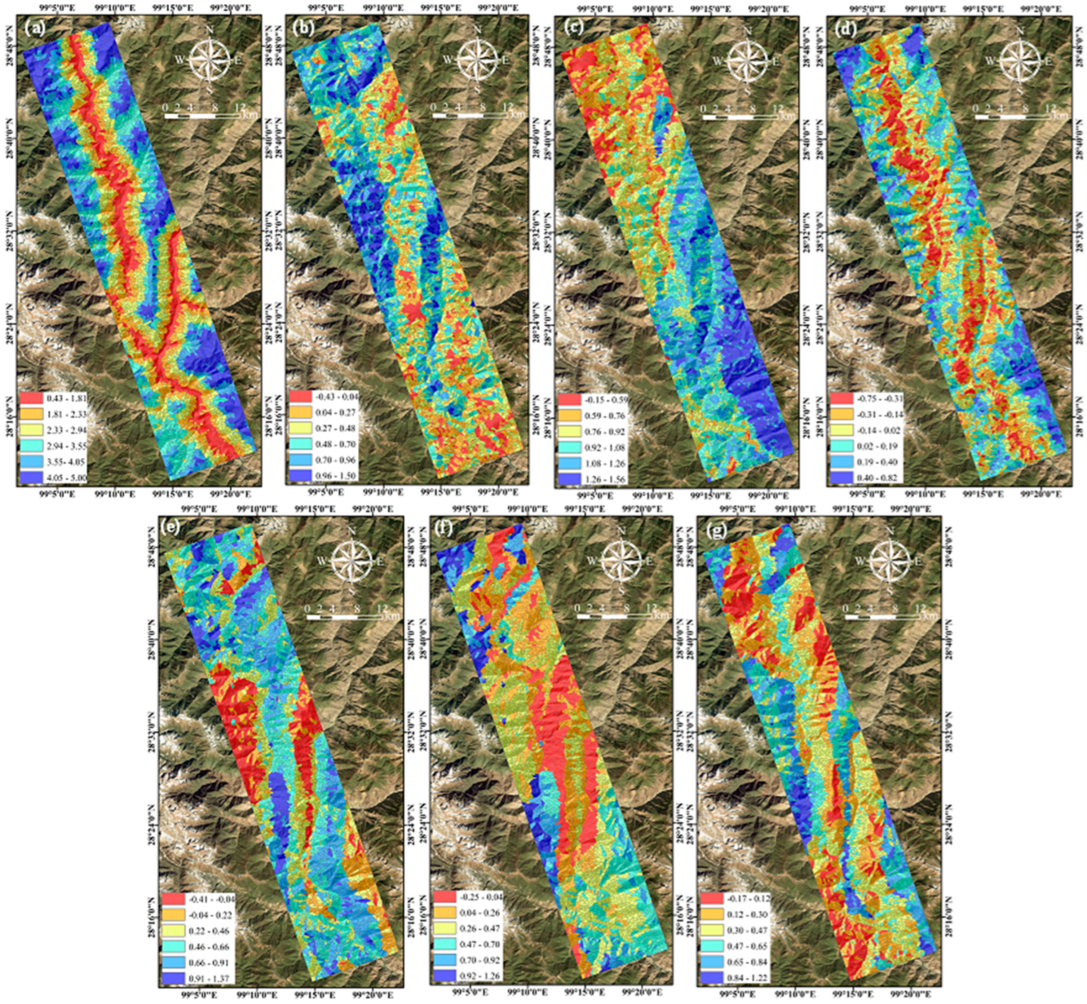
Per PCA method guidelines, the Kaiser–Meyer–Olkin (KMO) and Bartlett’s tests were run first on evaluation index values from slope units before principal component analysis was conducted. Results showed a KMO score of 0.764, with Bartlett’s test yielding 48,271.116 and a significance level of 0.000. Generally, a KMO value over 0.7 makes principal component analysis viable. Here, the KMO score for slope unit-derived evaluation indices exceeded 0.7, pointing to strong collinearity and justifying the use of principal component analysis. In calculating the correlation matrix’s maximum eigenvalues, those above 0.75 were selected as principal components, resulting in seven such components (Figure 8) with a cumulative variance exceeding 80%. This means that these seven components hold more than 80% of the original evaluation indices’ information.

4.3. Result of Model Fitting

The PC1-PC7 values of both landslide and non-landslide samples were extracted, and these samples were randomly split into five equal subsets. For modeling purposes, landslide units were labeled as 1 and non-landslide units as 0 to form the target layer. The SVM was chosen due to its demonstrated effectiveness in landslide susceptibility mapping [1,20]. Crucially, we applied identical SVM parameters (RBF kernel, C = 0.8, g = 0.5) to both sampling methods, ensuring that the observed performance differences solely stem from our novel sampling strategy, not algorithmic tuning. The model fitting results are shown in Figure 9.

5. Discussion

5.1. Model Comparison

After training and testing with various non-landslide samples, ROC curves were drawn for the five-fold cross-validation modeling results, and their corresponding AUC values were calculated. As shown in Figure 9, when using randomly selected non-landslide samples, the model had an average AUC of 0.882 in training and 0.878 in testing. For non-landslide samples randomly selected from the low/very low-susceptibility areas of the landslide susceptibility map derived by the CF method, the average AUCs in the training and testing stages were 0.924 and 0.920, respectively. In terms of ROC standard deviation, the modeling results using non-landslide samples from the low/very low regions of the CF-based susceptibility map had a smaller standard deviation than those using randomly selected non-landslide samples in both training and testing. This highlights the significant performance advantage of the CF-guided sampling strategy.
Models utilizing non-landslide samples randomly picked from at least 200 m away from landslides produced training and testing AUC values of 0.882 and 0.878, respectively. In comparison, sampling from CF-derived low/very low-susceptibility zones resulted in notably higher AUC values of 0.924 (training) and 0.920 (testing), marking a 4.8% improvement in accuracy. Importantly, both methods displayed a minimal difference between training and testing AUC values (ΔAUC = 0.004), indicating strong generalization ability. Additionally, the CF approach reduced the ROC standard deviation by 32% in testing (Figure 9), confirming enhanced model stability. These findings clearly demonstrate that CF can be effectively repurposed as a spatial filter for sample selection, rather than being limited to a factor-weighting tool.
The accuracy gains stem from resolving a fundamental limitation in conventional LSM modeling. Random sampling risks including geologically unstable areas within “non-landslide” training data [2], introducing false negatives that blur decision boundaries. Our CF-guided approach circumvents this by leveraging geostatistical prior knowledge to identify true stable zones, particularly slopes with low curvature (>−0.2), distal from faults (>2 km), and in resistant lithologies (e.g., DTJ ophiolite). This physical preprocessing creates a purified training dataset where SVM can establish sharper classification hyperplanes.

5.2. Model Comparison with Other Studies

Numerous scholars have conducted extensive research to develop a reasonable landslide susceptibility zoning map for the study area (Table 2). This paper further confirms the significance of non-landslide sample selection by comparing it with other modeling methods applied in the same area. To find slope units suitable for creating the study area’s landslide susceptibility map, Sun et al. [1] used both the hydrological analysis approach and the curvature watershed method to split the slope units within the study area. For the outcomes of these two division methods, they utilized an SVM model to create the landslide susceptibility zoning map. The results showed that the hydrological analysis method had average prediction accuracies of 0.897 during training and 0.881 during testing. On the other hand, the curvature watershed method achieved average prediction accuracies of 0.907 during training and 0.890 during testing. This indicates that the slope units divided by the curvature watershed method are better than those divided by hydrological analysis method.
Seeking to refine landslide susceptibility models suited to the study area, Sun et al. (2022) [30] ran susceptibility modeling analyses using logistic regression (LR), random forest (RF), and artificial neural network (ANN) models, all built on slope units. Their findings showed that the LR model hit average prediction accuracies of 0.857 (training) and 0.852 (testing). The RF model reached 0.964 and 0.870 in training and testing phases, while the ANN model scored 0.910 and 0.890, respectively. That said, every one of these models relied on randomly picking non-landslide units during setup, ignoring how non-landslide sample selection methods affect landslide susceptibility mapping.
Therefore, to verify the influence of non-landslide unit selection on landslide susceptibility zoning, this paper chose two non-landslide unit sample selection methods to build the study area’s landslide susceptibility zoning model. The CF-SVM framework (with a testing AUC of 0.920) outperformed (a) SVM based on hydrological slope units (AUC = 0.881 [1]); (b) ANN models with random sampling (AUC = 0.890 [30]); (c) logistic regression ensembles (AUC = 0.852 [30]); and (d) an RF model with random sampling (AUC = 0.870 [30]). This demonstrates that optimizing sample quality through physical heuristics is more effective than relying solely on algorithmic sophistication. Although deep learning approaches (such as ANN and RF) can achieve comparable accuracy, they require significantly more data and computational resources—a major limitation in data-scarce mountainous regions like the study area. Our method achieves superior performance using only 575 landslide units and 7 principal components. Therefore, making sound choices enhance the predictive precision of landslide susceptibility zoning models. This, in turn, offers useful direction for disaster prevention and mitigation initiatives in the upper reaches of the Jinsha River.

5.3. Landslide Susceptibility Map Analysis

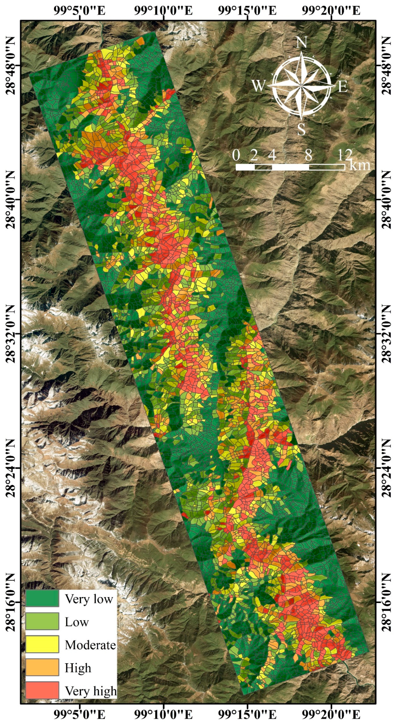
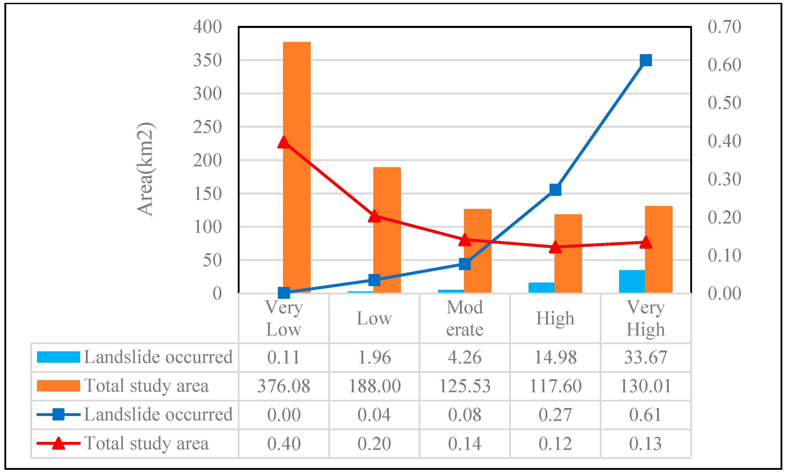
From modeling the outcomes of non-landslide samples randomly picked from the low/very low-susceptibility zones of the CF method-divided landslide susceptibility map, the model with the stronger predictive power was selected. This model was used to produce the study area’s final landslide susceptibility map, as shown in Figure 10. Statistical analysis was performed on this map, with the findings displayed in Figure 11. The data reveals that high- and very high-susceptibility areas in the map account for 25.70% of the study area’s total expanse. However, these zones hold 88.49% of the known landslide area, indicating that the landslide susceptibility zoning map is quite rational.
The study area’s landslide susceptibility map shows that areas with very high, high, and moderate susceptibility are mainly clustered in villages along the banks of the Jinsha River and Dingqu River. These villages have dense populations, high densities of buildings and farmland, and some industrial development, so they need to be given priority in disaster mitigation and prevention efforts. In contrast, low- and very low-susceptibility areas are mostly located in regions far from the Jinsha River and Dingqu River. Human activities here are relatively sparse, so even if landslides occur, the potential damage will be smaller; however, disaster prevention and mitigation measures are still needed. This spatial distribution emphasizes the importance of targeted risk management strategies. Due to their high vulnerability and socioeconomic exposure, villages in high-susceptibility areas need integrated planning that combines engineering and non-engineering measures. At the same time, remote areas with lower susceptibility should focus on basic monitoring and community preparedness to deal with residual risks, ensuring that disaster reduction efforts cover the entire study area comprehensively.

6. Conclusions

This study investigated landslide susceptibility mapping in the Upper Jinsha River region by comparing different non-landslide sampling methods. The objective was to optimize modeling accuracy and support disaster mitigation efforts. The main findings are as follows:
(a) The certainty factor (CF) is no longer just a factor evaluator; it now acts as a sample filter. We use the CF to mark true stable zones (with low and very low susceptibility) for non-landslide sampling. This fixes the big problem of random sampling, which often includes unstable units. This change has proven effective: it boosts AUC by 4.8% compared to random sampling. It shows that adding geological prior knowledge to data preparation works better than improving the algorithms.
(b) The CF-SVM framework is accurate and practical. It obtained a 0.920 testing AUC. It only used 575 landslide units and 7 principal components. It outperforms more complex models in the same region, like ANN (0.890 AUC) and RF (0.870 AUC). This makes it valuable for areas with little data, where deep learning is not possible.
(c) The susceptibility map offers useful risk mitigation guidance. A total of 88.49% of landslides are in 25.70% of the area. Most of these are along villages by the Jinsha and Dingqu Rivers. High- and very high-susceptibility zones gather in these densely populated villages. So, these places need top-priority engineering and non-engineering mitigation strategies. Low-risk areas are less vulnerable, but they still need basic monitoring to handle the remaining risk.
However, the CF-SVM framework for landslide susceptibility mapping has limitations: the “CF < 0.1” threshold for non-landslide sampling via the natural breaks method may have subjective bias across different geological backgrounds, and the SVM model is less capable of capturing complex nonlinear interactions between landslide-triggering factors compared to advanced models. Future improvements could integrate deep learning models, such as using CNNs or LSTMs, to process high-resolution spatiotemporal data for the dynamic characterization of landslide-prone conditions or develop hybrid frameworks like CF-UNet/CF-Transformer to enhance the learning of intricate geological patterns, especially in data-scarce mountainous regions like the upper Jinsha River.

Author Contributions

Conceptualization, Xin Zhou; methodology, Xin Zhou and Xiulei Li; software, Xin Zhou; validation, Yiding Bao; formal analysis, Xin Zhou and Xiulei Li; investigation, Xiaohui Sun and Ke Jin; resources, Yunkai Ruan, Xin Zhou, and Yiding Bao; data curation, Xin Zhou; writing—original draft preparation, Xin Zhou; writing—review and editing, Xiaohui Sun, Xin Zhou, Yunkai Ruan, Yiding Bao, Li Tang, and Xiulei Li. All authors have read and agreed to the published version of the manuscript.

Funding

This research was funded by the youth project of science and technology research program of Chongqing Education Commission of China (Grant No. KJ202200774654381); the National Natural Science Foundation of China (Grant No. 42007261); the Natural Science Foundation of Chongqing, China (Grant Nos. cstc2021jcyj-msxmX0869 and cstb2023nscq-msX0841); the Natural Science Foundation of Fujian Province, China (Grant No. 2021J05026); and the Open Project of Key Laboratory of Hydraulic and Waterway Engineering of the Ministry of Education, Chongqing Jiaotong University (Grant Nos. SLK2023B08 and SLK2021B09).

Data Availability Statement

Data supporting this research article are available from the corresponding author on request.

Acknowledgments

The authors would like to thank the editor and anonymous reviewers for their comments and suggestions, which helped a lot in improving this paper.

Conflicts of Interest

The authors declare no conflicts of interest.

References

  1. Sun, X.; Chen, J.; Han, X.; Bao, Y.; Zhou, X.; Peng, W. Landslide susceptibility mapping along the upper Jinsha River, south-western China: A comparison of hydrological and curvature watershed methods for slope unit classification. Bull. Eng. Geol. Environ. 2020, 79, 4657–4670. [Google Scholar] [CrossRef]
  2. Ozturk, U.; Pittore, M.; Behling, R.; Roessner, S.; Andreani, L.; Korup, O. How robust are landslide susceptibility estimates? Landslides 2021, 18, 681–695. [Google Scholar] [CrossRef]
  3. Sun, X.; Chen, J.; Bao, Y.; Han, X.; Zhan, J.; Peng, W. Landslide Susceptibility Mapping Using Logistic Regression Analysis along the Jinsha River and Its Tributaries Close to Derong and Deqin County, Southwestern China. ISPRS Int. J. Geo-Inf. 2018, 7, 438. [Google Scholar] [CrossRef]
  4. Thiery, Y.; Malet, J.P.; Sterlacchini, S.; Puissant, A.; Maquaire, O. Landslide susceptibility assessment by bivariate methods at large scales: Application to a complex mountainous environment. Geomorphology 2007, 92, 38–59. [Google Scholar] [CrossRef]
  5. Wang, S.; Lin, X.; Qi, X.; Li, H.; Yang, J. Landslide susceptibility analysis based on a PSO-DBN prediction model in an earthquake-stricken area. Front. Environ. Sci. 2022, 10, 912523. [Google Scholar] [CrossRef]
  6. Pourghasemi, H.R.; Rossi, M. Landslide susceptibility modeling in a landslide prone area in Mazandarn Province, north of Iran: A comparison between GLM, GAM, MARS, and M-AHP methods. Theor. Appl. Climatol. 2017, 130, 609–633. [Google Scholar] [CrossRef]
  7. Wu, Y.; Ke, Y.; Chen, Z.; Liang, S.; Zhao, H.; Hong, H. Application of alternating decision tree with AdaBoost and bagging ensembles for landslide susceptibility mapping. CATENA 2020, 187, 104396. [Google Scholar] [CrossRef]
  8. Lucchese, L.V.; de Oliveira, G.G.; Pedrollo, O.C. Attribute selection using correlations and principal components for artificial neural networks employment for landslide susceptibility assessment. Environ. Monit. Assess. 2020, 192, 129. [Google Scholar] [CrossRef]
  9. Dieu Tien, B.; Tran Anh, T.; Klempe, H.; Pradhan, B.; Revhaug, I. Spatial prediction models for shallow landslide hazards: A comparative assessment of the efficacy of support vector machines, artificial neural networks, kernel logistic regression, and logistic model tree. Landslides 2016, 13, 361–378. [Google Scholar] [CrossRef]
  10. Zhan, W.; Baise, L.G.; Moaveni, B. An uncertainty quantification framework for logistic regression based geospatial natural hazard modeling. Eng. Geol. 2023, 324, 107271. [Google Scholar] [CrossRef]
  11. Wang, G.; Chen, X.; Chen, W. Spatial Prediction of Landslide Susceptibility Based on GIS and Discriminant Functions. ISPRS Int. J. Geo-Inf. 2020, 9, 144. [Google Scholar] [CrossRef]
  12. Sahana, M.; Sajjad, H. Evaluating effectiveness of frequency ratio, fuzzy logic and logistic regression models in assessing landslide susceptibility: A case from Rudraprayag district, India. J. Mt. Sci. 2017, 14, 2150–2167. [Google Scholar] [CrossRef]
  13. Youssef, K.; Shao, K.; Moon, S.; Bouchard, L.S. Landslide susceptibility modeling by interpretable neural network. Commun. Earth Environ. 2023, 4, 162. [Google Scholar] [CrossRef]
  14. Huang, Y.; Zhao, L. Review on landslide susceptibility mapping using support vector machines. CATENA 2018, 165, 520–529. [Google Scholar] [CrossRef]
  15. Park, S.-J.; Lee, C.-W.; Lee, S.; Lee, M.-J. Landslide Susceptibility Mapping and Comparison Using Decision Tree Models: A Case Study of Jumunjin Area, Korea. Remote Sens. 2018, 10, 1545. [Google Scholar] [CrossRef]
  16. Polykretis, C.; Chalkias, C.; Ferentinou, M. Adaptive neuro-fuzzy inference system (ANFIS) modeling for landslide susceptibility assessment in a Mediterranean hilly area. Bull. Eng. Geol. Environ. 2019, 78, 1173–1187. [Google Scholar] [CrossRef]
  17. Achu, A.L.; Aju, C.D.; Di Napoli, M.; Prakash, P.; Gopinath, G.; Shaji, E.; Chandra, V. Machine-learning based landslide susceptibility modelling with emphasis on uncertainty analysis. Geosci. Front. 2023, 14, 101657. [Google Scholar] [CrossRef]
  18. Tang, L.; Liu, G.; Sun, X.; Liu, P. Optimizing storage-based reservoir operation schemes for enhanced large-scale hydrological modeling: A comprehensive sensitivity analysis. J. Hydrol. 2025, 657, 133173. [Google Scholar] [CrossRef]
  19. Wang, F.; Xu, P.; Wang, C.; Wang, N.; Jiang, N. Application of a GIS-Based Slope Unit Method for Landslide Susceptibility Mapping along the Longzi River, Southeastern Tibetan Plateau, China. ISPRS Int. J. Geo-Inf. 2017, 6, 172. [Google Scholar] [CrossRef]
  20. Sun, X.; Yu, C.; Li, Y.; Rene, N.N. Susceptibility Mapping of Typical Geological Hazards in Helong City Affected by Volcanic Activity of Changbai Mountain, Northeastern China. ISPRS Int. J. Geo-Inf. 2022, 11, 344. [Google Scholar] [CrossRef]
  21. Ali, N.; Chen, J.; Fu, X.; Ali, R.; Hussain, M.A.; Daud, H.; Hussain, J.; Altalbe, A. Integrating Machine Learning Ensembles for Landslide Susceptibility Mapping in Northern Pakistan. Remote Sens. 2024, 16, 988. [Google Scholar] [CrossRef]
  22. Liu, C.; Li, W.; Wu, H.; Lu, P.; Sang, K.; Sun, W.; Chen, W.; Hong, Y.; Li, R. Susceptibility evaluation and mapping of China’s landslides based on multi-source data. Nat. Hazards 2013, 69, 1477–1495. [Google Scholar] [CrossRef]
  23. Oliveira, S.C.; Zezere, J.L.; Garcia, R.A.C.; Pereira, S.; Vaz, T.; Melo, R. Landslide susceptibility assessment using different rainfall event-based landslide inventories: Advantages and limitations. Nat. Hazards 2024, 120, 9361–9399. [Google Scholar] [CrossRef]
  24. Guo, X.; Fu, B.; Du, J.; Shi, P.; Chen, Q.; Zhang, W. Applicability of Susceptibility Model for Rock and Loess Earthquake Landslides in the Eastern Tibetan Plateau. Remote Sens. 2021, 13, 2546. [Google Scholar] [CrossRef]
  25. Zhao, Z.; Liu, Z.Y.; Xu, C. Slope Unit-Based Landslide Susceptibility Mapping Using Certainty Factor, Support Vector Machine, Random Forest, CF-SVM and CF-RF Models. Front. Earth Sci. 2021, 9, 589630. [Google Scholar] [CrossRef]
  26. Jennifer, J.J.; Saravanan, S. Artificial neural network and sensitivity analysis in the landslide susceptibility mapping of Idukki district, India. Geocarto Int. 2022, 37, 5693–5715. [Google Scholar] [CrossRef]
  27. Quan, H.-C.; Lee, B.-G. GIS-based landslide susceptibility mapping using analytic hierarchy process and artificial neural network in Jeju (Korea). KSCE J. Civ. Eng. 2012, 16, 1258–1266. [Google Scholar] [CrossRef]
  28. Kim, J.-C.; Lee, S.; Jung, H.-S.; Lee, S. Landslide susceptibility mapping using random forest and boosted tree models in Pyeong-Chang, Korea. Geocarto Int. 2018, 33, 1000–1015. [Google Scholar] [CrossRef]
  29. Wang, X.; Nie, W.; Xie, W.; Zhang, Y. Incremental learning-random forest model-based landslide susceptibility analysis: A case of Ganzhou City, China. Earth Sci. Inform. 2024, 17, 1645–1661. [Google Scholar] [CrossRef]
  30. Sun, X.; Chen, J.; Li, Y.; Rene, N.N. Landslide Susceptibility Mapping along a Rapidly Uplifting River Valley of the Upper Jinsha River, Southeastern Tibetan Plateau, China. Remote Sens. 2022, 14, 1730. [Google Scholar] [CrossRef]
  31. Sun, X.; Han, X.; Chen, J.; Bao, Y.; Peng, W. Numerical simulation of the Qulong Paleolandslide Dam event in the late pleistocene using the finite volume type shallow water model. Nat. Hazards 2022, 111, 439–464. [Google Scholar] [CrossRef]
  32. Sun, X.; Chen, J.; Han, X.; Bao, Y.; Zhan, J.; Peng, W. Application of a GIS-based slope unit method for landslide susceptibility mapping along the rapidly uplifting section of the upper Jinsha River, South-Western China. Bull. Eng. Geol. Environ. 2020, 79, 533–549. [Google Scholar] [CrossRef]
  33. Rossi, M.; Guzzetti, F.; Reichenbach, P.; Mondini, A.C.; Peruccacci, S. Optimal landslide susceptibility zonation based on multiple forecasts. Geomorphology 2010, 114, 129–142. [Google Scholar] [CrossRef]
  34. Cao, C.; Wang, Q.; Chen, J.; Ruan, Y.; Zheng, L.; Song, S.; Niu, C. Landslide Susceptibility Mapping in Vertical Distribution Law of Precipitation Area: Case of the Xulong Hydropower Station Reservoir, Southwestern China. Water 2016, 8, 270. [Google Scholar] [CrossRef]
  35. Kumar, C.; Walton, G.; Santi, P.; Luza, C. An Ensemble Approach of Feature Selection and Machine Learning Models for Regional Landslide Susceptibility Mapping in the Arid Mountainous Terrain of Southern Peru. Remote Sens. 2023, 15, 1376. [Google Scholar] [CrossRef]
  36. Kumar, D.; Thakur, M.; Dubey, C.S.; Shukla, D.P. Landslide susceptibility mapping & prediction using Support Vector Machine for Mandakini River Basin, Garhwal Himalaya, India. Geomorphology 2017, 295, 115–125. [Google Scholar] [CrossRef]
  37. Sharma, S.; Mahajan, A.K. A comparative assessment of information value, frequency ratio and analytical hierarchy process models for landslide susceptibility mapping of a Himalayan watershed, India. Bull. Eng. Geol. Environ. 2019, 78, 2431–2448. [Google Scholar] [CrossRef]
  38. Sun, X.; Chen, J.; Bao, Y.; Han, X.; Zhan, J.; Peng, W. Flash flood schlep ability estimation in vertical distribution law of the precipitation area: A case of Xulong gully, Southwest China. Arab. J. Geosci. 2019, 12, 279. [Google Scholar] [CrossRef]
  39. Sun, X.; Liu, G.; Zhao, T.; Tang, L.; Han, X.; Peng, W. Application of a geomorphic restoration method for landslide susceptibility mapping along the rapidly uplifting section of the upper Jinsha river, South-Western China. Bull. Eng. Geol. Environ. 2025, 84, 181. [Google Scholar] [CrossRef]
  40. Cao, B.; Li, Q.; Zhu, Y. Comparison of Effects between Different Weight Calculation Methods for Improving Regional Landslide Susceptibility-A Case Study from Xingshan County of China. Sustainability 2022, 14, 11092. [Google Scholar] [CrossRef]
  41. Chen, Z.; Quan, H.; Jin, R.; Jin, A.; Lin, Z.; Jin, G.; Jin, G. Assessment of Landslide Susceptibility Using the PCA and ANFIS with Various Metaheuristic Algorithms. KSCE J. Civ. Eng. 2024, 28, 1461–1474. [Google Scholar] [CrossRef]
  42. Dey, S.; Das, S.; Roy, S.K. Landslide susceptibility assessment in Eastern Himalayas, India: A comprehensive exploration of four novel hybrid ensemble data driven techniques integrating explainable artificial intelligence approach. Environ. Earth Sci. 2024, 83, 641. [Google Scholar] [CrossRef]
  43. Chen, W.; Chai, H.; Zhao, Z.; Wang, Q.; Hong, H. Landslide susceptibility mapping based on GIS and support vector machine models for the Qianyang County, China. Environ. Earth Sci. 2016, 75, 474. [Google Scholar] [CrossRef]
  44. Chen, S.; Pan, Y.; Lu, C.; Wang, Y.; Wu, M.; Pedrycz, W. Landslide spatial prediction based on cascade forest and stacking ensemble learning algorithm. Int. J. Syst. Sci. 2025, 56, 658–670. [Google Scholar] [CrossRef]
  45. Costache, R.; Ali, S.A.; Parvin, F.; Quoc Bao, P.; Arabameri, A.; Hoang, N.; Craciun, A.; Duong Tran, A. Detection of areas prone to flood-induced landslides risk using certainty factor and its hybridization with FAHP, XGBoost and deep learning neural network. Geocarto Int. 2022, 37, 7303–7338. [Google Scholar] [CrossRef]
  46. Qin, Y.; Yang, G.; Lu, K.; Sun, Q.; Xie, J.; Wu, Y. Performance Evaluation of Five GIS-Based Models for Landslide Susceptibility Prediction and Mapping: A Case Study of Kaiyang County, China. Sustainability 2021, 13, 6441. [Google Scholar] [CrossRef]
  47. Lin, G.-F.; Chang, M.-J.; Huang, Y.-C.; Ho, J.-Y. Assessment of susceptibility to rainfall-induced landslides using improved self-organizing linear output map, support vector machine, and logistic regression. Eng. Geol. 2017, 224, 62–74. [Google Scholar] [CrossRef]
  48. Huang, F.; Yin, K.; Huang, J.; Gui, L.; Wang, P. Landslide susceptibility mapping based on self-organizing-map network and extreme learning machine. Eng. Geol. 2017, 223, 11–22. [Google Scholar] [CrossRef]
  49. Mandal, S.; Mandal, K. Bivariate statistical index for landslide susceptibility mapping in the Rorachu river basin of eastern Sikkim Himalaya, India. Spat. Inf. Res. 2018, 26, 59–75. [Google Scholar] [CrossRef]
  50. Mandal, S.P.; Chakrabarty, A.; Maity, P. Comparative evaluation of information value and frequency ratio in landslide susceptibility analysis along national highways of Sikkim Himalaya. Spat. Inf. Res. 2018, 26, 127–141. [Google Scholar] [CrossRef]
  51. Wang, Z.; Ma, C.; Qiu, Y.; Xiong, H.; Li, M. Refined Zoning of Landslide Susceptibility: A Case Study in Enshi County, Hubei, China. Int. J. Environ. Res. Public Health 2022, 19, 9412. [Google Scholar] [CrossRef] [PubMed]
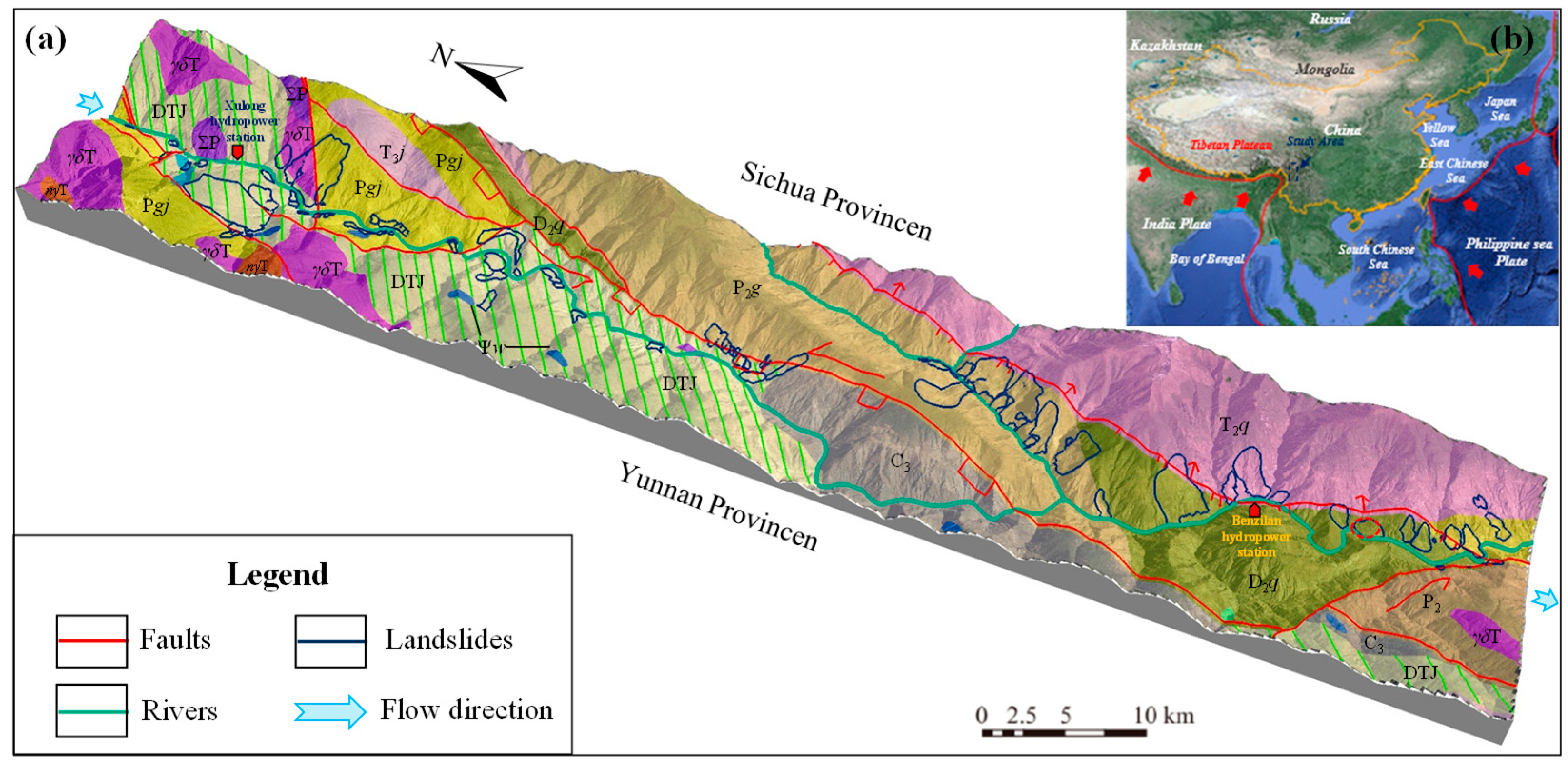
Figure 1. Location map of the study area: (a) geological map of the study area; (b) the location of the study area.
Ijgi 14 00339 g001
Figure 2. Flow chart of the study.
Ijgi 14 00339 g002
Figure 3. Typical unstable slope: (a) glacial till; (b) scattered huge boulders; (c) a typical landslide; (d) unstable deposits.
Ijgi 14 00339 g003
Figure 4. Slope unit division flow chart [1].
Ijgi 14 00339 g004
Figure 5. Landslide conditioning factors maps: lithological factors, including lithology (a) and rock hardness (b); topographic factors, including elevation (c), slope angle (d), slope aspect (e), topographic relief (f), and curvature (g); vegetation factors, including land use (h) and normalized difference vegetation index (NDVI) (i); geological structural factors, including distance from faults (j); terrain uplift factors, including Strahler’s integral value (k); river factors, including distance from rivers (l); rainfall, including rainfall (m); seismic factor, including earthquake intensity (n).
Ijgi 14 00339 g005aIjgi 14 00339 g005b
Figure 6. Slope unit division result map of the study area: (a) slope unit division result; (b) landslide susceptibility map using CF; (c) random non-landslide sample set; (d) low/very low-susceptibility random non-landslide sample set.
Ijgi 14 00339 g006
Figure 7. The result of CF value calculation of conditioning factors correlation analysis.
Ijgi 14 00339 g007
Figure 8. Outcomes of principal component (PC) extraction: (a) PC 1; (b) PC 2; (c) PC 3; (d) PC 4; (e) PC 5; (f) PC 6; (g) PC7.
Ijgi 14 00339 g008
Figure 9. The performance percentages of landslide susceptibility models fitted to slope units: (a) random non-landslide sample set; (b) low/very low-susceptibility random non-landslide sample set.
Ijgi 14 00339 g009
Figure 10. Landslide susceptibility map.
Ijgi 14 00339 g010
Figure 11. Statistical results of the landslide susceptibility map.
Ijgi 14 00339 g011
Table 1. Landslide conditioning factors in the present study.
Conditioning FactorsData SourceVariable TypeMutator Methods of the
Slope Units
LithologyDepartment of Geological Survey
(1:200,000 scale)
CategoricalMajor value
Rock hardness
ElevationDigital elevation model
(91 Weitu software, 8.96 m)
ContinuesAverage value
Slope angle
Slope aspect
Topographic relief
Curvature
Land useLandsat 5 TM images
(3 April 2015)
CategoricalMajor value
NDVIContinuesAverage value
Distance from faultsDepartment of Geological Survey
(1:200,000 scale)
Strahler’s integral valueSun et al., 2020 [1]
Distance from riversDepartment of Geological Survey
(1:200,000 scale)
RainfallSun et al. 2019 [30]
Earthquake intensitySun et al. 2025 [39]CategoricalMajor value
Table 2. Model fitting outcomes across various studies in the research region.
SourceMethodPrediction AccuracyMapping Unit
This studySVM
Non-landslide samples randomly selected
Training0.882Slope units
Testing0.878
SVM
Non-landslide samples randomly selected from the low- and very low-susceptibility regions of the CF-based landslide susceptibility map
Training0.924
Testing0.920
(Sun et al., 2020) [1]SVM
Hydrologic method
Training0.897
Testing0.881
SVM
Curvature watershed method
Training0.907
Testing0.890
(Sun et al., 2022) [30]LRTraining0.857
Testing0.852
RFTraining0.964
Testing0.870
ANNTraining0.910
Testing0.890
Disclaimer/Publisher’s Note: The statements, opinions and data contained in all publications are solely those of the individual author(s) and contributor(s) and not of MDPI and/or the editor(s). MDPI and/or the editor(s) disclaim responsibility for any injury to people or property resulting from any ideas, methods, instructions or products referred to in the content.