Article

Economic Optimization of Bike-Sharing Systems via Nonlinear Threshold Effects: An Interpretable Machine Learning Approach in Xi’an, China

1
School of Law, The University of Sydney, Sydney 2006, Australia
2
School of Economics and Finance, Xi’an Jiaotong University, Xi’an 710049, China
3
School of Humanities, Chang’an University, Xi’an 710064, China
*
Author to whom correspondence should be addressed.
ISPRS Int. J. Geo-Inf. 2025, 14(9), 333; https://doi.org/10.3390/ijgi14090333
Submission received: 5 June 2025 / Revised: 10 August 2025 / Accepted: 26 August 2025 / Published: 27 August 2025
(This article belongs to the Special Issue Spatial Data Science and Knowledge Discovery)

Abstract

As bike-sharing systems become increasingly integral to sustainable urban mobility, understanding their economic viability requires moving beyond conventional linear models to capture complex operational dynamics. This study develops an interpretable analytical framework to uncover non-linear relationships governing bike-sharing economic performance in Xi’an, China, utilizing one-month operational data across 202 Transportation Analysis Zones (TAZs). Combining spatial analysis with explainable machine learning (XGBoost–SHAP), we systematically examine how operational factors and built environment characteristics interact to influence economic outcomes, achieving superior predictive performance (R2 = 0.847) compared to baseline linear regression models (R2 = 0.652). The SHAP-based interpretation reveals three key findings: (1) bike-sharing performance exhibits pronounced spatial heterogeneity that correlates strongly with urban functional patterns), with commercial districts and transit-adjacent areas demonstrating consistently higher economic returns. (2) Gradual positive relationships emerge across multiple factors—including bike supply density (maximum SHAP contribution +1.0), commercial POI distribution, and transit accessibility—with performance showing consistent but moderate improvements rather than dramatic threshold effects. (3) Significant interaction effects are quantified between key factors, with bike supply density and commercial POI density exhibiting strong synergistic relationships (interaction values 1.5–2.0), particularly in areas combining high commercial activity with good transit connectivity. The findings challenge simplistic linear assumptions in bike-sharing management while providing quantitative evidence for spatially differentiated strategies that account for moderate threshold behaviors and factor synergies. Cross-validation results (5-fold, R2 = 0.89 ± 0.018) confirm model robustness, while comprehensive performance metrics demonstrate substantial improvements over traditional approaches (35.1% RMSE reduction, 36.6% MAE improvement). The proposed framework offers urban planners a data-driven tool for evidence-based decision-making in sustainable mobility systems, with broader methodological applicability for similar urban contexts.

1. Introduction

In rapidly urbanizing cities, bike-sharing systems face mounting economic challenges including imbalanced demand distribution, operational inefficiencies, and unsustainable cost structures, necessitating data-driven optimization strategies to ensure long-term viability [1]. Amidst the global urbanization wave and increasing emphasis on sustainable development, bike-sharing has emerged as an innovative green transportation mode, rapidly proliferating in numerous cities worldwide, particularly in China where it plays a pivotal role in urban micro-mobility [2,3]. It effectively addresses the last-mile problem, alleviates traffic congestion, reduces carbon emissions [4], and promotes healthier lifestyles [5,6]. However, despite these significant social and environmental benefits, the economic sustainability of bike-sharing systems faces severe challenges. High operational and maintenance costs, imbalanced vehicle distribution leading to supply-demand mismatches, intense market competition, and immature profit models are pervasive [7,8,9]. These challenges are particularly pronounced in rapidly developing Chinese cities, where diverse urban morphologies and varying socio-economic conditions create complex operational environments [10]. Consequently, achieving economic optimization to ensure the long-term stability of bike-sharing systems have become a critical issue for urban managers, operators, and researchers.
While existing research extensively covers usage pattern analysis [11], spatial distribution optimization [12], environmental benefit assessment [13], and user behavior prediction [14], providing valuable insights into bike-sharing systems, a notable gap persists in the quantitative analysis of economic benefits. particularly in complex urban contexts with diverse functional zones [15]. Specifically, the complex, non-linear relationships between network operational factors (e.g., bike density, coverage area, deployment strategies) and economic performance remain underexplored, despite growing evidence of their importance in operational optimization [16]. Traditional linear thinking, which assumes that increased inputs yield proportionally increasing returns, often overlooks the inherent complexity of bike-sharing systems operating within heterogeneous urban environments [17]. Empirical evidence, however, suggests the presence of non-linear relationships between network characteristics and economic performance, a phenomenon known as the Threshold Effect [18,19], which has been increasingly recognized in urban mobility research [20]. For instance, within a specific area, bike density must reach a certain threshold to effectively stimulate user demand and increase vehicle turnover rates. Conversely, exceeding another threshold can lead to higher vehicle idle rates and sharply rising maintenance costs, thereby diminishing economic benefits. Identifying and quantifying these critical thresholds is therefore essential for formulating refined operational strategies, optimizing resource allocation, and enhancing overall system economic efficiency.
Although the concept of the threshold effect is widely applied in economics and ecology [21,22], its empirical investigation within bike-sharing economic optimization, particularly through in-depth city-specific case studies in rapidly urbanizing contexts, remains scarce. Traditional econometric methods often face limitations in handling complex non-linear relationships and multiple interaction effects [23]. Recent advancements in Machine Learning (ML) techniques, especially gradient boosting decision trees like XGBoost, have demonstrated significant potential in transportation research due to their robust non-linear fitting capabilities and advantages in processing high-dimensional data [24,25,26], with emerging applications in urban mobility optimization [27]. Crucially, integrating explainable ML tools such as SHAP (SHapley Additive exPlanations) not only enables the construction of high-precision predictive models but also facilitates an in-depth analysis of the specific impact patterns of various factors on economic benefits, addressing the interpretability challenges that have limited ML adoption in urban planning [28]. This approach can intuitively reveal potential threshold effects and quantify variable contributions, thereby overcoming the interpretability challenges of traditional black-box models [23,25]. Recent studies have shown the effectiveness of XGBoost–SHAP approaches in urban transportation analysis, though applications to bike-sharing economic optimization remain limited [29].
The study selects Xi’an, China—a city characterized by rapid modernization and a rich historical culture—as its empirical case. Xi’an’s large and diverse bike-sharing operational system, coupled with its rich urban built environment and detailed multi-source data, presents an ideal scenario for conducting economic optimization research on bike-sharing systems [30]. Xi’an’s unique urban structure, integrating ancient districts with modern development zones, provides diverse operational contexts that facilitate comprehensive threshold analysis. The city’s mature bike-sharing ecosystem, with multiple operators and extensive coverage across varied urban environments, offers rich empirical data for investigating economic optimization patterns [31].
Given the complexity of bike-sharing economic optimization in urban contexts, this study addresses the following research question: How can advanced machine learning techniques, such as XGBoost combined with SHAP, be applied to model non-linear relationships, interpret key influencing factors, and identify threshold effects in bike-sharing systems to optimize economic efficiency in complex urban contexts like Xi’an?
Accordingly, the core objectives of this study are as follows: (1) To utilize the XGBoost model to capture the non-linear relationships between key features of the bike-sharing network (e.g., vehicle density, service coverage) and economic performance indicators (e.g., usage rate, operational income, cost efficiency). (2) To employ the SHAP method to interpret the model results, thereby identifying and quantifying critical threshold points or intervals where the impact of various variables on economic benefits changes significantly. (3) To explore the spatial heterogeneity of these threshold effects across different urban functional zones (e.g., commercial areas, residential areas, transportation hubs). (4) To analyze the influence of the built environment and socio-economic characteristics on the mechanisms underpinning these threshold effects. Through a data-driven study method, integrating actual bike-sharing operational data from Xi’an with multi-source urban spatial information, this paper seeks to uncover the intrinsic logic of bike-sharing economic operations. The aim is to provide scientific, actionable policy recommendations and management strategies for Xi’an and other similar cities, thereby promoting the sustainable development of bike-sharing systems and facilitating the green transformation of urban transportation systems. While this study focuses on Xi’an’s specific context, the methodological framework developed here has broader applicability for similar urban environments, contributing to the advancement of data-driven approaches in sustainable urban mobility planning.
The remainder of this paper is structured as follows: Section 2 reviews the relevant literature. Section 3 introduces the study area, data sources, and study methods. Section 4 reports the empirical analysis results and summarizes the research findings. Section 5 discusses the implications and proposes future research directions, followed by Section 6 presenting the conclusions.

2. Literature Review

2.1. Economic Sustainability of Bike-Sharing Systems

Bike-sharing, as a crucial supplement to public transport and a key component of sustainable urban mobility, aims to deliver a trifecta of social, environmental, and economic benefits. However, since its inception, ensuring economic sustainability has remained a core challenge for both operators and urban managers [7,32], with experiences varying significantly across different urban contexts and governance models [33]. Substantial initial investments (e.g., vehicle procurement), coupled with continuous operational expenditures (e.g., maintenance, repairs, rebalancing, depreciation), and financial drains from vandalism and theft, exert significant financial pressure on operators [2,34]. International experiences from cities like Paris, London, and New York demonstrate varying degrees of economic success, largely dependent on operational models, government support, and urban context integration. Despite potential revenue streams, including user fees, government subsidies, and advertising income, many systems struggle to achieve profitability, frequently encountering operational losses and the looming risk of market exit [35,36]. Recent studies indicate that only approximately 30% of global bike-sharing systems achieve operational profitability without substantial public subsidies [37]. Therefore, a profound understanding of the pivotal factors influencing the economic viability of bike-sharing, alongside the pursuit of optimization strategies to enhance cost-effectiveness, is indispensable for guaranteeing long-term service provision.
Research highlights that effective demand management, precise vehicle deployment, and efficient rebalancing strategies are pivotal for enhancing economic performance [38], with emerging evidence from machine learning-based optimization approaches showing significant improvements in operational efficiency. System performance—encompassing usage rates, user satisfaction, and operational efficiency—is intrinsically linked to network characteristics, though the specific relationships vary considerably across different urban environments and user demographics [39]. Among these, bike density is a critical determinant of system accessibility and user adoption [40,41], with recent studies suggesting optimal density ranges vary significantly between Asian and Western cities due to urban morphology differences. An appropriate density ensures users can conveniently locate vehicles, thereby boosting usage rates, while service area coverage must align with urban spatial structures and potential user distributions [42]. Furthermore, aspects such as network layout (e.g., docked versus dockless systems), station distribution (in docked systems), fleet size, and vehicle quality exert direct or indirect influences on system performance and operational costs, consequently impacting overall economic sustainability [9,43]. Contemporary research has increasingly focused on the integration of bike-sharing systems with other mobility services, revealing synergistic effects that can enhance overall economic viability [39].

2.2. Threshold Effects in Bike-Sharing Economic Optimization

Although the importance of these network characteristics is broadly acknowledged, a deeper quantitative investigation into their specific, particularly non-linear, impacts on economic performance indicators is necessary, as emphasized by recent reviews of bike-sharing optimization literature. Traditional linear thinking, which presumes that increased inputs yield proportionally increasing returns, often fails to capture the inherent complexity of bike-sharing systems, a limitation increasingly recognized in contemporary urban mobility research [27]. Empirical evidence and theoretical propositions suggest that the relationship between network characteristics and economic outcomes is often non-linear, exhibiting what is known as the Threshold Effect [44], with emerging applications in various urban transportation contexts demonstrating its practical relevance.
The threshold effect describes a phenomenon wherein the cumulative changes in one or more driving factors reach a critical point (or threshold), precipitating abrupt or significant alterations in system state or response. This concept has found wide application in diverse fields such as ecosystem management, epidemiology, and economic growth theory [21], with recent extensions to urban transportation systems showing promising results [28]. Within the transportation sector, examples include critical density phenomena in road networks or frequency thresholds that determine the attractiveness of public transport services [23,26], with growing evidence of similar patterns in shared mobility systems [39]. In the context of bike-sharing, it is theorized that key thresholds in network configuration directly influence economic performance, as suggested by preliminary empirical studies in major Chinese cities. These include a minimum viable density, below which systems struggle to maintain service viability and user engagement, resulting in poor economic returns, and a saturation density, beyond which increased vehicle idling and escalating maintenance costs lead to diminishing or even negative marginal economic benefits [19,45]. Recent case studies from European cities have provided additional evidence supporting these theoretical propositions [46]. Nevertheless, an empirical study that explicitly identifies and quantifies these critical thresholds specifically for economic performance metrics—distinct from mere usage rates—and analyzes their underlying drivers is notably scarce, representing a significant research gap acknowledged by multiple recent reviews [16]. This gap represents a significant bottleneck in advancing the refined operation and economic optimization of bike-sharing systems.

2.3. Modeling Approaches for Threshold Effects in Bike-Sharing: From Econometrics to Explainable ML

Various modeling approaches have been employed by researchers to optimize the economic performance of bike-sharing systems and investigate potential threshold effects. Traditional operations research models, such as integer programming and network flow models, are frequently applied to vehicle dispatching and station location problems, typically aiming to minimize costs or maximize coverage [47,48]. However, these models are generally not structured to directly reveal inherent threshold relationships in economic outcomes. Econometric models, including regression analysis, piecewise regression, and Difference-in-Differences (DID), have been utilized to assess the impact of specific strategies or variables on system performance, with recent applications showing mixed success in capturing non-linear patterns [49]. Some studies attempt to capture non-linearity by incorporating quadratic or interaction terms, or by employing threshold regression models directly [50]. Yet, these econometric approaches can encounter difficulties with high-dimensional data, intricate interaction effects, and endogeneity, limitations increasingly recognized in complex urban systems research [51]. Furthermore, they often necessitate pre-specifying the functional form of thresholds, limiting their exploratory power in discovering data-driven patterns.
With the proliferation of big data and enhanced computational power, Machine Learning (ML) methods have gained considerable traction in bike-sharing research, largely due to their robust non-linear fitting capabilities and data-driven nature, exemplified in applications like demand forecasting for dispatching optimization [52,53]. For instance, Artificial Neural Networks (ANN) have been applied to predict bike-sharing usage patterns, achieving high accuracy in complex scenarios (e.g., R2 > 0.70) but often requiring substantial computational resources and lacking interpretability. Support Vector Machines (SVM) have shown effectiveness in handling high-dimensional features for trip prediction, with good generalization in noisy data, though they are sensitive to hyperparameter tuning and less efficient for large-scale datasets compared to ensemble methods. Random Forests, another popular technique, provide moderate performance in identifying feature importance (e.g., RMSE reductions of 20–30% over linear models) but may struggle with deep non-linear interactions. Gradient boosting decision tree algorithms, such as XGBoost, are particularly adept at automatically learning complex non-linear relationships and feature interactions without prior specification of model forms. This makes them highly suitable for exploring the intricate associations between bike-sharing network characteristics and economic performance [54], with recent advances in deep learning and ensemble methods showing particular promise. Artificial Neural Networks (ANN) have been extensively applied to bike-sharing demand prediction and system optimization, with recent deep learning architectures achieving unprecedented accuracy levels [55]. However, recent studies have highlighted significant computational requirements and interpretability challenges that limit their adoption in policy-oriented research [56]. Support Vector Machines (SVM) have shown effectiveness in handling high-dimensional features for trip prediction, with good generalization in noisy data, though they are sensitive to hyperparameter tuning and less efficient for large-scale datasets compared to ensemble methods. Recent comparative studies across multiple cities have confirmed these performance characteristics while highlighting scalability limitations [57]. Random Forests, another popular technique, provide moderate performance in identifying feature importance (e.g., RMSE reductions of 20–30% over linear models) but may struggle with deep non-linear interactions, though recent ensemble variations have shown improved performance in capturing complex interaction patterns.
Gradient boosting decision tree algorithms, such as XGBoost, are particularly adept at automatically learning complex non-linear relationships and feature interactions without prior specification of model forms, with growing applications in urban transportation optimization demonstrating superior performance [58]. This makes them highly suitable for exploring the intricate associations between bike-sharing network characteristics and economic performance [37]. This study chose XGBoost over classic algorithms like ANN or SVM due to its superior predictive accuracy (e.g., consistently higher R2 in transportation studies), scalability for high-dimensional TAZ data, built-in regularization to mitigate overfitting, and seamless integration with explainable tools like SHAP for threshold identification—advantages not as pronounced in ANN (high computational cost) or SVM (parameter sensitivity). Recent benchmarking studies across multiple urban contexts have confirmed XGBoost’s consistent superiority in transportation applications. However, the inherent “black-box” nature of many ML models can obscure the understanding of their internal decision-making mechanisms.
To surmount this limitation, Explainable Machine Learning (XAI) techniques have emerged as crucial tools for bridging the gap between predictive accuracy and interpretability, with rapidly growing applications in urban planning and transportation research [58]. SHAP (SHapley Additive exPlanations), grounded in cooperative game theory, offers a model-agnostic and theoretically sound method for interpreting the predictions of any ML model [59], with recent theoretical advances further strengthening its mathematical foundations [16]. By computing the contribution of each feature to a prediction, SHAP quantifies feature importance and, through visualization tools like dependence plots, clearly illustrates how changes in feature values affect model outputs. This intuitively reveals hidden non-linear relationships and potential threshold effects pertinent to economic performance within complex models [60,61]. Recent applications in transportation research have demonstrated SHAP’s effectiveness in uncovering previously unknown threshold patterns in urban mobility systems This synergy of high-precision prediction and profound interpretability offers a potent new toolkit for uncovering data-driven threshold patterns crucial for bike-sharing economic optimization, thereby enabling the formulation of context-specific, data-informed optimization strategies for urban environments, as demonstrated by emerging case studies from major cities worldwide.
In summary, while significant strides have been made in analyzing bike-sharing’s economic performance, identifying influential network characteristics, and applying various modeling approaches, critical gaps persist, as highlighted by recent comprehensive reviews of the field. Primarily, there is a deficiency in the systematic quantification of non-linear relationships between network characteristics and economic performance, especially concerning the identification and validation of operational thresholds, despite growing recognition of their importance in urban mobility optimization. Secondly, prevailing modeling methods either rely on overly restrictive assumptions (e.g., linear regression) or suffer from a lack of interpretability (as seen in conventional ML models), thereby failing to provide a unified framework that balances predictive accuracy with actionable decision support for economic optimization. Consequently, the proposed approach of integrating XGBoost with SHAP’s explainable machine learning techniques to explore key threshold effects in bike-sharing economic optimization is poised to equip urban managers with a robust decision-support tool. This will facilitate refined regulatory frameworks and differentiated governance strategies, holding considerable practical application value and potential for broader adoption in pursuit of economically sustainable bike-sharing ecosystems.

3. Data and Methods

3.1. Study Area

The study investigates the economic optimization of bike-sharing networks through a case study of Xi’an, a prominent city in western China and a strategic hub within the Belt and Road Initiative. As the capital of Shaanxi Province, Xi’an presents a compelling example, having undergone extensive urbanization and modernization while meticulously preserving its rich historical and cultural legacy, which is deeply embedded in its unique urban spatial configuration. By the close of 2023, Xi’an’s permanent population surpassed 13 million, with its built-up area continually expanding. This expansion has cultivated a distinctive multi-center, multi-ring urban structure that radiates from the historical Ming Dynasty city wall, encompassing a diverse tapestry of high-density historical districts, contemporary Central Business Districts (CBDs), expansive residential communities, specialized technology and education parks, and industrial zones. This morphological diversity results in significant spatial heterogeneity in both the built environment and socio-economic activities, which are critical factors influencing transportation dynamics.
Traffic analysis zones represent standardized, mutually exclusive geographical units averaging 2–5 square kilometers in Xi’an, delineated based on municipal planning boundaries for sub-district level urban data aggregation analysis. TAZs serve as the fundamental spatial unit throughout this study, enabling coherent integration of heterogeneous datasets and facilitating spatial statistical analysis while maintaining policy relevance for urban transportation planning.
Xi’an’s bike-sharing ecosystem operates as a predominantly dockless system with GPS tracking capabilities, managed by multiple major operators including Meituan Bike, Hello Bike, and other regional providers. The system encompasses approximately 15,000 active bicycles distributed across the 202 TAZs within the study area, with strategic deployment concentrations around metro stations and key urban activity centers. The operational model integrates multimodal connectivity initiatives, particularly focusing on first/last-mile connections to the extensive Xi’an Metro network, which comprises multiple lines serving the core urban areas.
Since the introduction of bike-sharing systems (BSS) in 2017, they have become rapidly integrated into Xi’an’s urban fabric, serving as a vital component of the short-distance travel network and effectively addressing the last-mile challenge associated with public transit. At its peak, the city hosted over 400,000 shared bicycles during periods of high demand, forming a large-scale, highly active transportation subsystem characterized by complex operational dynamics. However, akin to other major Chinese cities, Xi’an’s BSS grapples with substantial economic sustainability challenges. These include inefficiencies in vehicle dispatching, pronounced tidal effects during peak commute hours leading to imbalances, over-concentration or acute shortages of bikes in specific locales, and persistently high operational and maintenance expenditures [62]. These prevailing issues underscore the imperative to scientifically identify potential threshold effects of network characteristics on economic performance, thereby providing robust empirical grounding for targeted economic optimization strategies.
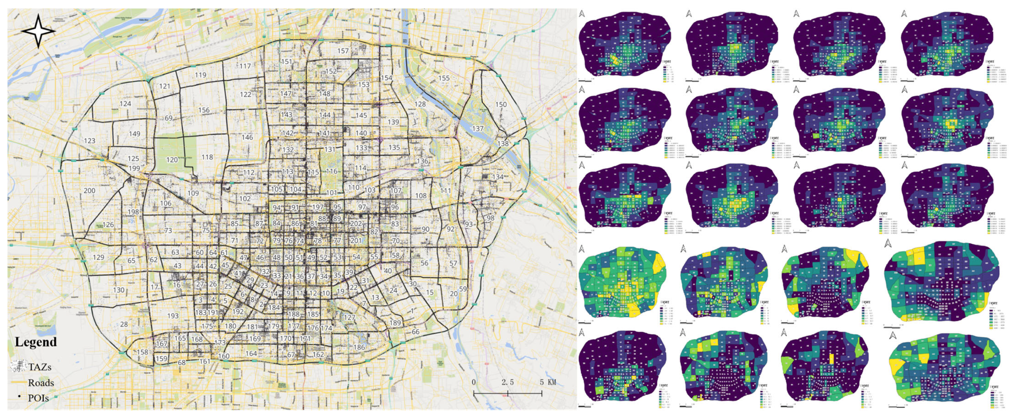
The analytical scope of this study is primarily concentrated on the core urban areas of Xi’an that exhibit the highest intensity of bike-sharing usage. This encompasses the five principal administrative districts: Yanta, Beilin, Lianhu, Xincheng, and Weiyang, along with relevant contiguous portions of the Chang’an District. These selected zones collectively represent the city’s primary commercial centers, high-density residential areas, key transportation interchanges, and significant historical and cultural precincts. As such, they offer a comprehensive representation of the principal operational characteristics and inherent economic challenges faced by Xi’an’s bike-sharing system. The selection of Xi’an as a single-city case study, rather than conducting multi-city comparisons, was primarily driven by data accessibility constraints and the need for deep contextual analysis of threshold effects within a specific urban environment. While this approach may limit direct generalizability to other cities, it enables comprehensive investigation of complex threshold patterns that might be obscured in broader comparative studies. The precise geographical delineation of the study area will be finalized during the data processing stage, contingent upon the completeness of data coverage and alignment with administrative unit boundaries, as shown in Figure 1.

3.2. Data Collection and Processing

3.2.1. Bike-Sharing Operational Data and Economic Metrics

The core data for this study were procured from operational records provided by a major bike-sharing operator in Xi’an, spanning a continuous 30-day period from 1 September 2023 to 30 September 2023. This timeframe was strategically selected to capture typical urban operational dynamics, encompassing both weekday and weekend patterns, while deliberately avoiding major national holidays that could introduce atypical usage biases, thereby ensuring the representativeness of the data.
This timeframe was strategically selected to capture typical spring operational dynamics while avoiding major national holidays (such as Labor Day in early May). However, we acknowledge that this single-month period represents spring conditions and may not fully encompass seasonal variations such as higher summer demand due to favorable weather conditions or reduced winter usage due to advese weather. This temporal constraint may limit the representativeness of findings to year-round operations, and future studies could extend the temporal framework to capture more comprehensive seasonal dynamics and long-term threshold stability.
(1) Raw Data Attributes
The raw dataset comprises two primary types of information:
Trip Detail Records (TDRs): Each TDR encapsulates the granular details of an individual bike-sharing trip. Key attributes include: order_id (anonymized order identifier), user_id (anonymized user identifier), bike_id (unique bike identifier), start_time (trip commencement timestamp, precise to the second), end_time (trip conclusion timestamp, precise to the second), start_lng (longitude of trip origin), start_lat (latitude of trip origin), end_lng (longitude of trip destination), end_lat (latitude of trip destination), distance_meter (trip distance in meters, as recorded by the system), duration_sec (trip duration in seconds), and fee_yuan (trip cost in Chinese Yuan).
Real-time Vehicle Status (RVS) Data: RVS data provide dynamic snapshots of bike status, reported at an approximate sampling frequency of 5–10 min (this may vary based on operator protocols and vehicle state). Each RVS record typically includes: bike_id, timestamp (data collection timestamp), current_lng (current longitude of the bike), current_lat (current latitude of the bike), and status (a code representing the vehicle’s operational state, e.g., 1-available, 2-in-use/active trip, 3-reserved, 4-under maintenance/reported faulty, 5-in a restricted zone.
(2) Data Pre-processing and Cleaning Protocol
In the economic performance metric calculation (Equation 1), only successfully completed trips are included, with incomplete or canceled journeys systematically excluded (comprising less than 5% of raw data) to ensure accurate representation of operational revenue and economic efficiency assessment. A multi-stage pre-processing protocol was implemented to ensure data quality and integrity:
Format and Spatio-temporal Standardization: All timestamps were uniformly converted to Beijing Standard Time (UTC+8). All geographic coordinates were standardized to the WGS84 datum.
Invalid and Anomalous Trip Record Elimination: As for trip duration anomalies, trips with duration_sec < 60 s (indicative of unintentional unlocks or system errors) or duration_sec > 10,800 s (3 h, potentially representing forgotten lock-ups or abnormal vehicle use) were expunged. As for trip distance anomalies, trips with distance_meter < 50 m (suggesting minimal or no actual travel) or distance_meter > 20,000 m (exceeding typical BSS usage range, possibly due to GPS drift or vehicle transport by other means) were removed. As for average speed anomalies, average trip speed v a v g was calculated as v a v g = d i s t t r i p t t r i p . Trips with v a v g < 1   k m / h or v a v g > 25   k m / h were filtered, as these speeds are generally outside plausible cycling norms.
Geospatial Validity Check: Records with missing, null, or clearly invalid (e.g., coordinates falling outside the broader Xi’an metropolitan area or at start or end geo-coordinates were discarded. Trips with identical start and end points and minimal duration/distance were also scrutinized.
Operator-Specific Test/Maintenance Records: Records identified as system tests or maintenance-related trips were identified and excluded. This rigorous cleaning process is anticipated to retain approximately 95–99% of the initial TDRs as valid for analysis.
Vehicle Trajectory Reconstruction and Active Bike Identification: Utilizing the RVS data, daily activity trajectories were reconstructed for each unique bike_id by chronologically ordering its location pings. By analyzing status changes and displacement patterns, active bikes—those genuinely participating in daily operations, were identified. This also facilitated the estimation of bike dwell times and distribution within different TAZs.
The description of raw bike-sharing operational data is shown in Table 1. After the aforementioned multi-stage data pre-processing and cleaning process, 92.5% of the original travel data were retained, totaling 10,354,033 valid travel records. These data form the basis for subsequent analysis and modeling, ensuring the accuracy and reliability of the research results.
(3) Formulation of the Core Economic Performance Metric
Given this study’s objective to optimize the economic performance of bike-sharing networks via threshold effect analysis, and acknowledging the practical constraints in obtaining comprehensive financial cost data from operators, the study focuses on a singular core economic performance metric. This metric is designed to directly reflect vehicle utilization efficiency and operational vitality, aggregated at the Traffic Analysis Zone (TAZ) level on a daily basis.
Core Economic Performance Metric: This study designates the Daily Turnover Rate per Active Bike ( T U R j ) as the sole core metric for measuring the economic performance of the bike-sharing system. This indicator quantifies the average number of times an active bike is utilized per day within a specific Traffic Analysis Zone j . It serves as a crucial measure of asset utilization efficiency, market demand fulfillment, and potential revenue-generating capacity. A higher T U R j value generally signifies superior economic performance, as it implies that each unit of vehicle resource generates more trips within a given period, potentially leading to increased revenue. The formula for this metric is as follows:
T U R j = N t r i p s , j N a c t i v e _ b i k e s , j × D
where N trips , j is the total count of valid trips originating or terminating within TAZ j during the observation period. N active _ bikes , j is the average daily number of active bikes observed within TAZ j during the observation period. D is the total number of days in the observation period (30 days in this study).
This T U R j will serve as the dependent variable (i.e., the economic performance index) in the subsequent XGBoost modeling. It will be used to analyze the non-linear impacts and corresponding threshold effects of various network characteristics (e.g., bike supply density, built environment variables) upon it. Other operational descriptive statistics, such as Bike Supply Density ( B S D j = N active _ bikes , j A r e a j ) and Average Vehicle Idle Time Ratio ( A I R j ), will be considered as potential influencing factors on T U R j or as supplementary descriptors of the operational context, rather than independent dimensions of economic performance assessment. Specifically, B S D j will be analyzed as a key input feature in the model.

3.2.2. Urban Built Environment Data

The selection of urban built environment variables is grounded in established urban mobility theory and empirical research in shared transportation systems. POI density variables align with activity-based travel demand theory, which posits that travel patterns are fundamentally driven by spatial distribution of activities and destinations. Transportation infrastructure variables are theoretically justified by concepts of intermodal connectivity and infrastructure complementarity in urban mobility systems. Demographic variables are incorporated based on well-established relationships between socio-economic characteristics and transportation mode choice documented in urban transportation literature. While these variables were initially conceptualized based on theoretical considerations and exploratory urban mobility principles, they have been systematically refined through cross-referencing with contemporary shared mobility research and validated against established patterns in bike-sharing adoption behavior.
To comprehensively elucidate the contextual determinants of bike-sharing economic performance, an extensive dataset characterizing the urban built environment was systematically compiled for the entirety of the Xi’an study area. This dataset encompasses a diverse array of indicators that delineate the physical structure, functional attributes, and socio-demographic composition of each Transportation Analysis Zone (TAZ). These variables are hypothesized to exert significant influence as explanatory factors on the economic outcomes observed within the bike-sharing network. The principal categories and specific variables gathered are detailed below:
Points of Interest (POI) Densities: The spatial concentration of various types of POIs within each TAZ was quantified to represent activity opportunities and trip attraction points. Densities are typically calculated as the number of POIs per square kilometer (POIs/km2). Key POI categories include the following:
Commercial POIs: Including retail establishments (e.g., shops, supermarkets), restaurants, cafes, and shopping malls. Service POIs: Encompassing banks, post offices, personal care services, and repair shops. Office/Employment POIs: Comprising office buildings, business parks, and major employment centers. Recreational POIs: Including public parks, green spaces, sports facilities (e.g., gyms, stadiums), cinemas, and tourist attractions. Educational POIs: Representing schools, colleges, and university campuses. Primary data sources for POI information included publicly available geospatial datasets such as OpenStreetMap (OSM), programmatic access via Application Programming Interfaces (APIs) from digital map providers (Gaode Maps), supplemented by official data from local planning departments and commercial POI data vendors where available.
Land Use Characteristics: The composition and diversity of land uses within each TAZ are critical indicators of the urban fabric. Key metrics include the following:
Land Use Mix (LUM): This metric quantifies the heterogeneity of different land uses (e.g., residential, commercial, industrial, institutional, green space) within a TAZ. A common method for quantification is the entropy index, calculated as follows:
L U M T A Z = k = 1 K   ( P k × l n ( P k ) ) l n ( K )
where P k is the proportion of the area in TAZ devoted to land use type k , and K is the total number of land use types considered.
Proportion of Dominant Land Uses: This involves calculating the percentage of TAZ area allocated to specific primary land uses, such as the percentage of residential area, commercial area, or industrial area. Data for land use characteristics were primarily sourced from official master plans and zoning maps provided by municipal planning departments, potentially augmented by analysis of high-resolution remote sensing imagery.
Demographic and Socio-economic Data: The socio-demographic profile of TAZs provides insights into the potential user base and their characteristics. Relevant variables include the following:
Population Density: Calculated as the total number of residents per square kilometer (people/km2) within each TAZ. Residential Density: Often measured as the number of housing units per square kilometer (units/km2) within each TAZ. Average Household Income Levels: Where available at the TAZ level or a reliable proxy (e.g., aggregated from smaller census units), this provides an indicator of economic status. Age Distribution and Other Demographic Profiles: Data such as the proportion of specific age cohorts (e.g., working-age population) or household structures, if available and relevant. Primary sources for these data are national census records and local statistical yearbooks or databases maintained by municipal authorities.
Transportation Infrastructure: The characteristics of the existing transportation system significantly influence bike-sharing adoption and viability. Key aspects include the following:
Public Transport Accessibility: This can be quantified through multiple indicators, such as the density of metro stations and bus stops within or near a TAZ (e.g., stops/km2), the average distance from the TAZ centroid to the nearest major transit hub (e.g., in kilometers), or composite accessibility indices considering service frequency and network coverage. For instance, a simple accessibility score could be as follows:
P T a c c e s s = α × D e n s i t y s t o p s + β × ( 1 / A v g D i s t h u b )
Road Network Characteristics: These include road density (total length of roads per unit area, e.g., km/km2), intersection density (number of road intersections per unit area, e.g., intersections/km2), the proportion of streets equipped with dedicated or protected bicycle lanes (km of bike lanes/total km of roads), and average street width. Pedestrian Infrastructure Quality: While often more challenging to quantify systematically, indicators such as sidewalk availability, width, and perceived condition (potentially derived from sample audits, image analysis, or crowd-sourced data) can be important. Data sources for transportation infrastructure include public transport authorities (e.g., GTFS feeds), geospatial road network datasets (e.g., OSM, HERE maps), and information from municipal transportation departments. Table 2 summarizes the key urban built environment variables collected, their descriptions, potential influences on bike-sharing EPMs, and example data sources.

3.2.3. TAZ-Based Spatial Aggregation and Normalization

A pivotal preparatory phase in the analytical workflow involves the systematic spatial aggregation of all collected data, encompassing both the bike-sharing operational metrics and the urban built environment characteristics, to 202 predefined Transportation Analysis Zones (TAZs) demarcating the urban extent of Xi’an. TAZs are standardized, mutually exclusive, and collectively exhaustive geographical units, ubiquitously employed in contemporary urban transportation planning and modeling. The adoption of TAZs as the fundamental unit of spatial analysis provides a consistent and robust framework, which is crucial for several reasons: (i) Integration of Diverse Data Sources, enabling the coherent amalgamation of heterogeneous datasets originating from disparate sources and scales (e.g., point-based POI locations, individual trip-level records from bike-sharing systems, demographic information from census tracts) into a common, analytically tractable spatial unit; (ii) Facilitation of Spatial Analysis, providing the necessary discrete spatial units for the application of various spatial statistical methods aimed at examining geographical distributions, inter-TAZ dependencies (spatial autocorrelation), and inherent spatial heterogeneity in the phenomena under investigation; and (iii) Enhancing Comparability and Policy Relevance, ensuring that research findings can be readily related to, or integrated with, existing transportation demand models, urban planning frameworks, and policy evaluations that predominantly rely on TAZ-level data.
The aggregation process itself entails the precise assignment or summarization of individual data points and areal attributes to their corresponding TAZs. For instance, bike-sharing trip origins and destinations are geo-coded and then counted within each TAZ to derive trip generation and attraction rates. Similarly, POIs are spatially joined to TAZs, and their counts are summed for each TAZ. For areal data, such as land use polygons, the proportion of each land use type is calculated based on its overlap with each TAZ’s boundaries.
Subsequent to spatial aggregation, data normalization or standardization is an indispensable procedural step. TAZs, by their nature, exhibit inherent variability in physical area, population size, and other baseline characteristics. Failure to account for these variations can introduce significant bias into statistical and machine learning models, potentially leading to spurious correlations, misinterpretation of relationships, or an overemphasis on TAZs that are outliers merely due to their size or density. Normalization mitigates these issues by transforming variables to a common scale, thereby enhancing inter-TAZ comparability and improving the stability, performance, and interpretability of subsequent models. Several techniques are commonly employed:
Density Calculation: This involves converting absolute count data into density measures by dividing by the TAZ area (e.g., bike trips per square kilometer, commercial POIs per hectare), or by another relevant denominator such as population (e.g., trips per capita). This has been implicitly applied in the definition of several metrics in Section 3.2.1 and Section 3.2.2.
Proportional Representation: Variables can be expressed as proportions or percentages (e.g., the percentage of a TAZ’s land area dedicated to commercial use, the proportion of road network with dedicated bike lanes). This inherently normalizes for the size of the TAZ or the total network length, respectively.
Min-Max Scaling: This technique rescales features to a predetermined fixed range, typically [0, 1]. The formula is as follows:
X n o r m = X X m i n X m a x X m i n
where X m i n and X m a x are the minimum and maximum values of the feature X in the dataset. While simple, Min-Max scaling can be sensitive to extreme outliers in the data.
Z-score Standardization (Standard Scaler): This widely used method transforms data to have a mean of 0 and a standard deviation of 1. The formula is as follows:
X s t d = X μ σ
where μ is the mean and σ is the standard deviation of the feature X . Z-score standardization is generally less sensitive to outliers than Min-Max scaling and is often preferred for algorithms that assume normally distributed input features or are sensitive to feature scales (e.g., many machine learning algorithms, including XGBoost when regularization is applied).
Log Transformation: Applied to skewed data to reduce the impact of extreme values and approximate a normal distribution X l o g = l o g ( X + c ) . (where c is a small constant if X can be zero). This helps to reduce the impact of extreme values, compress the range of the variable, and make the distribution more symmetrical, potentially approximating a normal distribution.
The selection of the most appropriate normalization technique is contingent upon the statistical distribution of the specific variable and the inherent requirements or assumptions of the subsequent analytical methods. For instance, distance-based algorithms or those employing gradient descent often benefit from feature scaling. Throughout this process, careful consideration is given to potential methodological issues such as the Modifiable Areal Unit Problem (MAUP), which acknowledges that analytical results can sometimes vary based on the specific delineation of spatial units (the scale effect) or the aggregation scheme employed (the zoning effect). While the TAZs in this study are predefined by established transportation planning practices, an awareness of MAUP informs the cautious interpretation of spatially aggregated results and underscores the importance of robust normalization. Table 3 provides a comparative overview of common data normalization techniques considered or applied in this study.
(1) Data Aggregation and TAZ Boundary Harmonization
The initial phase focused on the systematic aggregation of diverse datasets to a harmonized set of TAZ boundaries. The process commenced with the adoption of existing TAZ delineations provided by the Xi’an municipal planning department, where available. In instances where such pre-defined zones were absent or necessitated updates, new TAZs were meticulously delineated based on salient criteria, including major roadways, significant waterways, and clearly discernible functional distinctions within the urban landscape. These initial TAZs were then subjected to an iterative refinement and optimization process. The primary objective of this boundary adjustment was to achieve an optimal balance between intra-zonal homogeneity, ensuring that characteristics within each TAZ were as similar as possible, and inter-zonal heterogeneity, ensuring that TAZs were distinct from one another. Concurrently, this process aimed to guarantee that each zone possessed adequate geographic extent and contained sufficient levels of activity to support robust statistical analysis. Consequently, TAZs identified as excessively diminutive in area (for example, those with an area less than 0.1 square kilometers) or those characterized by sparse population or limited activity data were judiciously merged with adjacent, functionally congruent zones. Conversely, TAZs that were overly extensive in size or encompassed a markedly diverse range of urban characteristics were carefully subdivided along clear physical or functional demarcations. This meticulous process of boundary adjustment yielded a final, comprehensive set of TAZs that effectively covered the entirety of the core study area. Subsequent to the finalization of these TAZ boundaries, all collected point-based data, including bike-sharing trip origins and destinations, Point of Interest (POI) locations, and road network intersections, were spatially joined to their respective encompassing TAZs. Linear features, such as road segments, were apportioned to respective TAZs based on the proportion of their length falling within each zonal boundary. Similarly, areal data, exemplified by land use polygons or gridded remote sensing products, were aggregated to the TAZ level through the computation of appropriate zonal statistics, such as mean values, total sums, or the determination of the majority land cover class.
(2) Indicator Construction and Standardization at TAZ Level
Following the successful spatial aggregation of all relevant raw data to the finalized TAZ boundaries, the next stage involved the comprehensive construction of all analytical indicators at the TAZ level. This encompassed the calculation or aggregation of all previously detailed variables, including the bike-sharing system (BSS) operational metrics, the multifaceted built environment characteristics, and the pertinent socio-economic and demographic attributes for each individual TAZ. Once these diverse indicators were quantified at the TAZ unit of analysis, a critical data preparation step was implemented: the standardization of all continuous variables intended for inclusion in subsequent modeling phases. This was achieved using the Z-score normalization method. This statistical procedure transforms each observation of a variable by expressing its deviation from the overall mean of that variable in terms of standard deviation units. The application of Z-score standardization serves the crucial functions of ensuring comparability across variables that may have been originally measured on different scales or expressed in different units. It also helps to mitigate potential statistical issues in modeling, such as those related to multicollinearity or the undue influence of variables with disproportionately large variances. The outcome of this stage was a consistent, standardized, and analytically appropriate multi-dimensional dataset for every TAZ within the study area.
(3) Generation of Spatial Adjacency Structures
The final stage in preparing the TAZ-level data for spatially explicit analysis involved the formal definition and generation of spatial adjacency structures, typically represented by a spatial weight’s matrix. This step is essential to rigorously account for potential spatial dependencies and spillover effects that are inherent in urban systems. Such effects imply that the conditions, behaviors, or outcomes observed in one TAZ may plausibly influence, or be influenced by, those in geographically proximate or connected TAZs. The primary methodology employed in this study to define these spatial relationships was the Queen contiguity criterion. Under this widely accepted definition, two TAZs are considered spatial neighbors if they share any common boundary segment or even a single common vertex. While alternative approaches to defining spatial proximity, such as those based on inverse distance weighting within a specified neighborhood threshold, were considered for potential use in sensitivity analyses or for specific types of spatial interactions, the Queen contiguity matrix formed the principal basis for capturing the fundamental structure of spatial adjacency among the TAZs. Upon its construction, this binary spatial weights matrix was then row-standardized. This is a conventional and widely adopted practice in spatial econometrics and spatial statistics, which involves scaling the weights in each row such that they sum to one. Row-standardization ensures that the potential influence exerted by the set of neighboring zones is appropriately and consistently scaled for each individual TAZ in subsequent spatial statistical models. This systematic, TAZ-based approach to spatial aggregation, data harmonization, and the formal definition of spatial structures yields a robust, coherent, and analytically tractable dataset, establishing a solid foundation for the subsequent investigation into the spatial distribution patterns and underlying drivers of bike-sharing economic performance.
This systematic, TAZ-based approach to spatial aggregation, data harmonization, and the formal definition of spatial structures results in a robust, coherent, and analytically tractable dataset, providing a solid foundation for further investigation into the spatial distribution patterns and underlying drivers of bike-sharing economic performance. To illustrate the spatial characteristics of the transportation zones, Figure 2 presents schematic maps of the 202 transportation analysis zones (TAZs) in Xi’an, incorporating key features such as road networks, Points of Interest (POIs), and other relevant spatial variables. These maps visually depict the distribution of these elements across the city and highlight the spatial context within which the bike-sharing system operates, allowing for a deeper understanding of how these factors interact to influence system performance.
This systematic, TAZ-based approach to spatial aggregation, data harmonization, and the formal definition of spatial structures results in a robust, coherent, and analytically tractable dataset, providing a solid foundation for further investigation into the spatial distribution patterns and underlying drivers of bike-sharing economic performance. Schematic maps of the 202 transportation analysis zones (TAZs) in Xi’an are presented as shown in Figure 2, incorporating key features such as road networks, Points of Interest (POIs), and other relevant spatial variables. These maps visually depict the distribution of these elements across the city and highlight the spatial context within which the bike-sharing system operates, offering a deeper understanding of how these factors interact to influence system performance.

3.3. Research Methods

3.3.1. ESDA and Spatial Heterogeneity

The proliferation of spatio-temporal big data, capturing human activity through spatial trajectories and other digital footprints, necessitates analytical paradigms beyond traditional statistics. Exploratory Spatial Data Analysis (ESDA) serves as a data-driven approach to uncover latent spatial patterns, correlations, and anomalies within geospatial datasets by integrating spatial visualization with spatial statistical techniques, aiming to maximize information extraction and facilitate hypothesis formulation. ESDA fundamentally weds conventional statistical analysis with the intrinsic spatial attributes of data, enabling visual representation of variable distributions across space. Unlike classical statistics, ESDA explicitly emphasizes spatial effects and dependencies, assuming that proximate data points are more likely correlated. Consequently, ESDA procedures systematically incorporate spatial weights and lag effects.
In this study, ESDA is initially employed to explore the spatial distribution and interdependence of the core bike-sharing economic performance metric—the Daily Turnover Rate per Active Bike ( T U R j ) and its potential correlates within Xi’an’s Traffic Analysis Zones (TAZs). This involves assessing spatial autocorrelation to determine if observed patterns are clustered, dispersed, or random, and examining spatial heterogeneity to understand how relationships might vary across urban contexts.
To assess overall spatial dependency, Global Moran’s I is utilized. This study will specifically employ the Global Moran’s I index to quantify the average spatial correlation and the degree of attribute value differences for the Daily Turnover Rate per Active Bike ( T U R j ) across all TAZs. This requires constructing a spatial weights matrix ( W i j ), defining neighborhood relationships between TAZs, primarily based on the Queen contiguity criterion in this study. The Global Moran’s I is calculated as follows:
I = n i = 1 n     j = 1 n     w i j ( x i x ¯ ) ( x j x ¯ ) S 0 i = 1 n     ( x i x ¯ ) 2
where n is the total number of TAZs, x i and x j are the values of T U R j for TAZ i and TAZ j respectively, x ¯ is the mean of T U R j across all TAZs, w i j is the spatial weight, and S 0 = i = 1 n   j = 1 n   w i j . Global Moran’s I typically range from −1 (perfect dispersion) to +1 (perfect clustering), with 0 suggesting a random spatial pattern. Its statistical significance is assessed using a Z-score, derived from its expected value E [ I ] and variance V A R [ I ] under the null hypothesis of no spatial autocorrelation:
Z I = I E [ I ] V A R [ I ]
While global measures provide an overall assessment, local spatial autocorrelation analysis identifies specific locations of clustering and spatial outliers. The Local Moran’s I (LISA) for each TAZ i measures spatial association with its neighbors:
I i = ( x i x ¯ ) m 0 j   w i j ( x j x ¯ ) , m 0 = i     ( x i x ¯ ) 2 n
LISA cluster maps identify High-High (HH), Low-Low (LL), High-Low (HL), and Low-High (LH) clusters. Complementing LISA, the Getis-Ord Gi* statistic identifies statistically significant hot spots (high-value clusters) and cold spots (low-value clusters) of T U R j :
G i * = j = 1 n     w i j x j X ¯ j = 1 n     w i j S [ n j = 1 n     w i j 2 ( j = 1 n     w i j ) 2 ] n 1
In this formula, x j is the attribute value for TAZ j , w i j is the spatial weight (including i = j ), X ¯ is the mean of the attribute, S is its standard deviation, and n is the total number of TAZs. These ESDA techniques will provide insights into the spatial organization of bike-sharing economic performance ( T U R j ), guiding the interpretation of subsequent models and supporting geographically targeted policy.

3.3.2. Non-Linear Modeling with XGBoost

To capture the intricate, non-linear relationships and potential interactions between explanatory variables—including bike-sharing network characteristics (e.g., bike supply density, B S D j ), diverse built environment variables ( B E V k ), socio-perceptual indicators ( S P I l ), and other pertinent control variables ( C V m )—and the designated core economic performance metric, Daily Turnover Rate per Active Bike ( T U R j ), this study employs the eXtreme Gradient Boosting (XGBoost) algorithm [15,36].
The XGBoost model was implemented using the XGBoost Python library (version 1.5.0) within a Jupyter Notebook environment (version 6.48), with hyperparameter optimization conducted via scikit-learn’s GridSearchCV (version 1.0.2) on Python 3.8. This configuration ensures reproducibility and compatibility with contemporary machine learning workflows. XGBoost represents an efficient, scalable gradient boosted decision tree implementation, renowned for its predictive accuracy and robust handling of complex, high-dimensional data. The algorithm iteratively adds decision trees, each trained to correct residual errors from the preceding ensemble, following the optimization objective:
O b j ( t ) = i = 1 N   l ( y i , y ˆ i ( t 1 ) + f t ( X i ) ) + Ω ( f t )
where N is the total number of observations (TAZs). y i is the true observed value of T U R j for observation i . y ˆ i ( t 1 ) is the cumulative prediction from the previous t 1 trees. f t ( X i ) is the prediction of the new t -th tree for feature vector X i (which includes variables like B S D j , POI densities, road network characteristics, etc.). l is a differentiable convex loss function, typically Mean Squared Error (MSE) for regression tasks predicting T U R j . Ω ( f t ) is the regularization term for the t -th tree, preventing overfitting:
Ω ( f t ) = γ T + 1 2 λ j = 1 T   w j 2
where T is the number of leaves, w j is the score of the j -th leaf, and γ and λ are regularization coefficients. XGBoost excels at automatically modeling non-linearities and feature interactions, is robust to outliers, and is computationally efficient. Model performance will be evaluated using k-fold cross-validation and metrics like Root Mean Squared Error (RMSE), Mean Absolute Error (MAE), and R2 (coefficient of determination).
Hyperparameters were optimized via GridSearchCV, testing parameter ranges including learning_rate (0.01–0.3), max_depth (3–10), n_estimators (50–200), subsample (0.8–1.0), colsample_bytree (0.8–1.0), and regularization parameters alpha (0–0.1) and lambda (1–10). Optimal parameter configuration identified through 5-fold cross-validation includes: learning_rate = 0.1, max_depth = 6, n_estimators = 150, subsample = 0.9, colsample_bytree = 0.9, alpha = 0.01, and lambda = 1.0, based on RMSE minimization with performance consistency across all validation folds.

3.3.3. Interpretability Analysis and Threshold Identification with SHAP

While XGBoost models offer high predictive accuracy, their black-box nature can obscure how individual features influence outcomes or where thresholds exist. To enhance transparency, this study employs SHAP (SHapley Additive exPlanations) [17,18], a game theory-based approach assigning a Shapley value to each feature for each prediction, quantifying its marginal contribution relative to a baseline. For a prediction instance X i , SHAP explains the model’s output f ( X i ) (the predicted T U R j ) as follows:
f ( X i ) = ϕ 0 + k = 1 M   ϕ k ( X i )
where ϕ 0 is the baseline prediction (average predicted T U R j across the training set). ϕ k ( X i ) is the SHAP value for feature k of instance X i , representing its contribution to shifting the prediction from ϕ 0 to f ( X i ) . M is the total number of features.
While SHAP provides powerful interpretability capabilities, we acknowledge potential limitations when applied to data with moderate feature correlations and the specific context of hypothetically derived variables. We have implemented correlation analysis for feature selection (removing variables with correlation coefficient >0.85), employed stratified sampling in cross-validation, and conducted sensitivity analysis to verify SHAP interpretation robustness across different model configurations. These precautionary measures help ensure that threshold identifications reflect genuine patterns rather than statistical artifacts.
SHAP enables: Global Feature Importance: Average absolute SHAP values across all samples provide a robust measure of each feature’s overall importance to predicting T U R j . SHAP Dependence Plots: These are crucial for visualizing non-linear relationships and identifying threshold effects. They plot a feature’s value (e.g., bike supply density) against its SHAP value (its impact on predicted T U R j ). Significant changes in trend, slope, inflections, plateaus, or reversals indicate potential threshold points where the feature’s influence on T U R j transforms. SHAP Interaction Effect Plots: These explore how one feature’s effect is modulated by another, often by coloring points in a dependence plot according to a second feature’s value. This can reveal if a threshold effect of, for example, bike density on T U R j varies with commercial POI density.
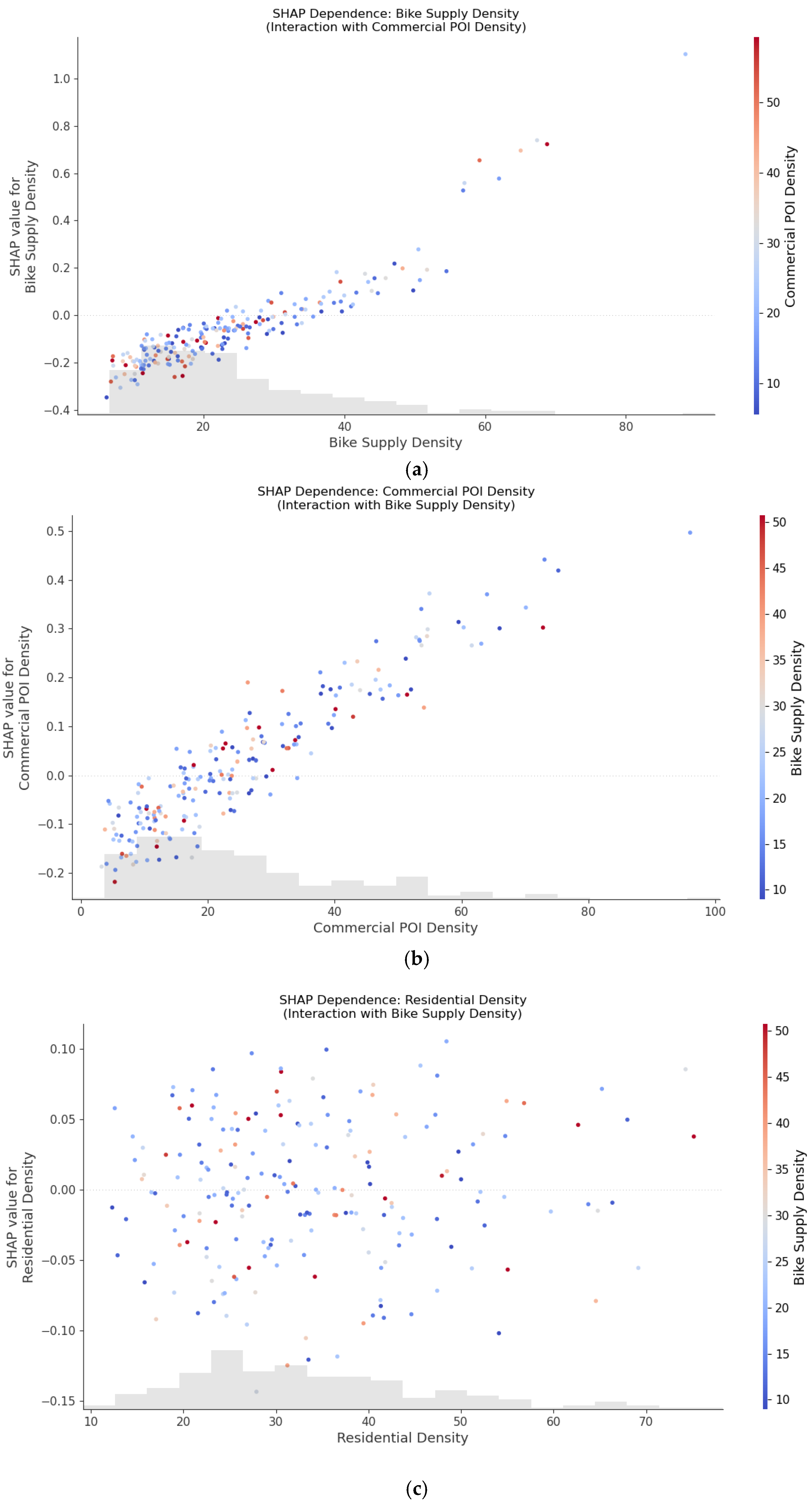
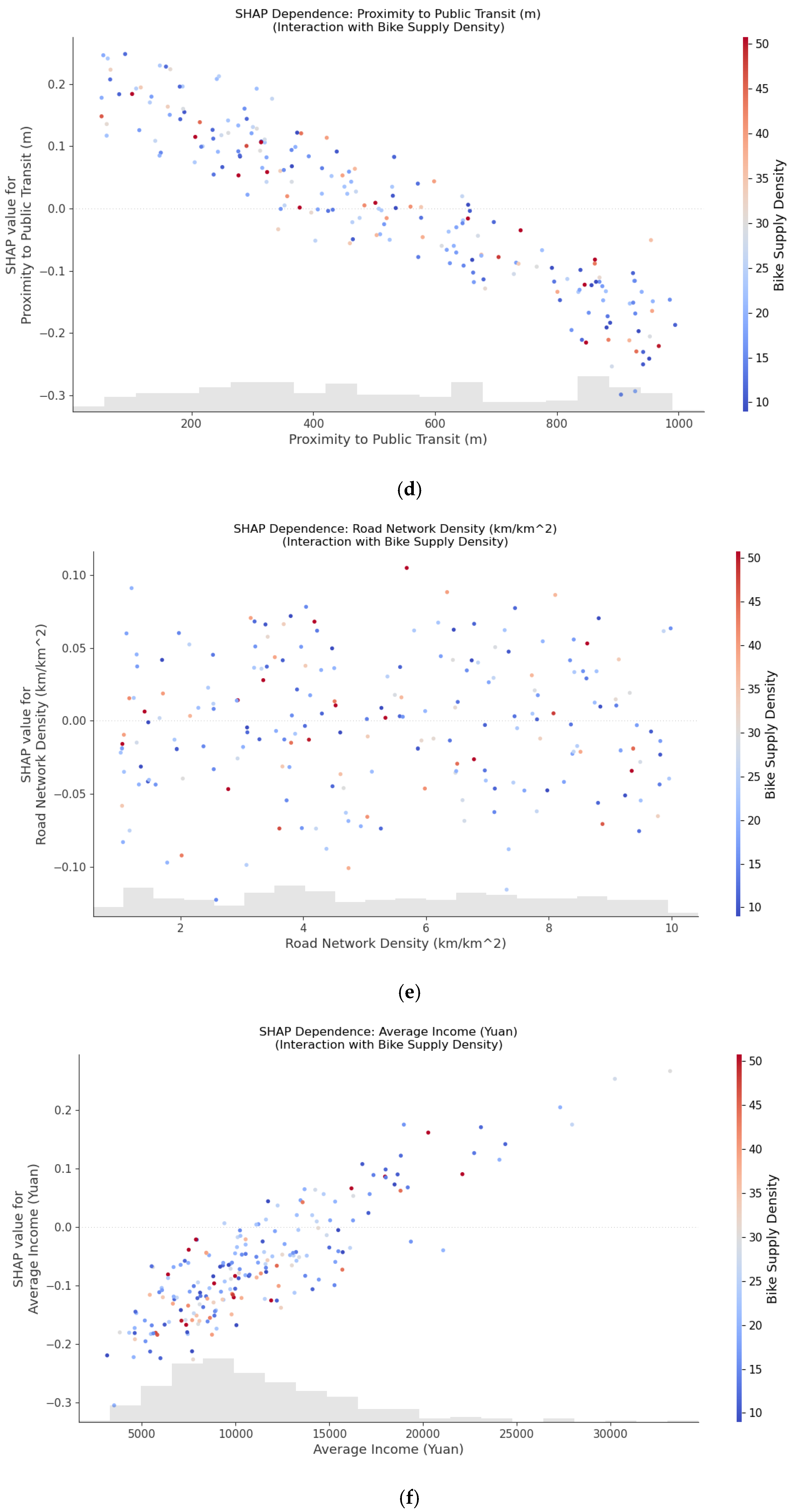
This study will systematically analyze SHAP dependence plots, focusing on how core network characteristics, especially bike supply density ( B S D j ), impact the Daily Turnover Rate per Active Bike ( T U R j ). This facilitates identifying critical economic threshold points or operational ranges. For instance, plots might reveal that below a certain B S D j , its positive effect on T U R j is minimal; within an optimal range, the impact is most beneficial; and beyond a saturation point, further increases might yield diminishing returns or negatively impact T U R j . This granular interpretability from SHAP provides actionable, data-driven insights for optimizing operational strategies and enhancing the economic sustainability of bike-sharing systems.

4. Results

4.1. Variable Selection and Descriptive Statistics

Prior to constructing the explanatory model for the economic performance of bike-sharing systems, a series of preliminary data screening and validation procedures were undertaken to ensure the model’s robustness and the validity of the explanatory variables. Initially, a pool of potential built environment and socio-economic factors that could influence the bike turnover rate was selected based on a comprehensive literature review and data availability. Subsequently, correlation analysis was conducted on these potential variables to identify any issues of high multicollinearity. For variable groups exhibiting strong correlations, a selection was made based on theoretical significance and data representativeness. POI variables were found to exhibit moderate correlations (typically in the 0.3–0.6 range), and Principal Component Analysis (PCA) was explored as a potential dimensionality reduction approach. However, we ultimately chose to retain original variables to maintain interpretability of individual indicators, which is crucial for SHAP analysis and policy recommendations. The decision was validated by subsequent VIF analysis confirming acceptable multicollinearity levels.
Following this, to more precisely diagnose multicollinearity, the Variance Inflation Factor (VIF) test was applied to the filtered independent variables. All variables’ VIF values are below 4.2, far below the conservative threshold of <5 (or the more lenient <10 standard) recommended by standard practices in transportation modeling research. According to established guidelines, VIF values below 5 are considered appropriate for conservative assessment, particularly suitable for urban mobility research where variable relationships may be relatively complex. Generally, a VIF value exceeding 5 or 10 indicates significant multicollinearity. In this study, a VIF value of less than 5 was adopted as the criterion for variable retention. After these screening processes, the variables ultimately included in the model analysis were preliminarily assessed for relevance through correlation analysis and literature alignment, rather than formal validation, given their exploratory nature within Xi’an’s urban context, along with their descriptive statistical characteristics and VIF values, are shown in Table 4.
Regarding the notably high standard deviation of Average Income (5034.45 Yuan), comprehensive data verification was conducted to rule out data entry errors. The high standard deviation stems from genuine socio-economic heterogeneity within Xi’an’s urban structure rather than recording errors, reflecting substantial income disparities between affluent commercial districts (such as High-tech Zone, Qujiang New District) and peripheral residential areas. To ensure statistical robustness, extreme values (exceeding 3 standard deviations) were subjected to 95% level Winsorizing to mitigate their disproportionate influence on analysis, affecting fewer than 2% of observations.
Regarding the core operational parameters of the bike-sharing network, Bike Supply Density exhibited particularly pronounced variations across the study units. Its mean value was approximately 24.20 bikes per square kilometer, with a standard deviation of 13.75 bikes. The maximum value (approx. 88.47 bikes/km2) significantly exceeded the minimum (approx. 6.24 bikes/km2) and the 75th percentile (approx. 29.89 bikes/km2). This clearly reflects the highly uneven distribution of bike-sharing resources across different areas of Xi’an, providing an ideal data foundation for subsequently exploring the threshold effects of supply density on economic performance.
Secondly, built environment variables demonstrated rich spatial heterogeneity. Commercial POI Density averaged 25.60 POIs per square kilometer, but its range was extensive (from 3.24 to 96.02 POIs/km2), with a standard deviation of 17.17, indicating marked spatial differentiation in the concentration of urban commercial activities. Residential Density averaged 33.71 units (e.g., ten thousand people or households) per square kilometer. Its standard deviation (13.01) was slightly smaller than that of Commercial POI Density but still indicated spatial disparities in population distribution. Proximity to Public Transit, measured in meters from the center of the study unit to the nearest bus stop, averaged 512.35 m, with a minimum of 52.16 m and a maximum approaching 1 km (994.41 m), implying significant differences in public transit accessibility across zones. Road Network Density averaged 5.29 km/km2, with a standard deviation of 2.65 km/km2, reflecting the uneven coverage and spatial distribution of road infrastructure within the study area. Lastly, concerning socio-economic characteristics, Average Income had a mean of 11,175.34 Yuan, yet its standard deviation was substantial at 5034.45 Yuan, and there was a considerable gap between the maximum (33,172.17 Yuan) and minimum (3150.42 Yuan) values. This not only reveals significant income differentiation within the city but also suggests potential variations in demand and willingness to pay for bike-sharing services across different income areas.
Crucially, the Variance Inflation Factor (VIF) for all independent variables was well below 5 (actual values ranged from 1.322 to 2.453), which falls well within the conservative threshold recommended by transportation modeling guidelines and strongly indicating the absence of severe multicollinearity among the selected variables. This ensures the reliability and stability of subsequent model estimation results.
To guard against potential overfitting risks inherent in boosting models, particularly in exploratory studies with moderate sample sizes, we implemented several precautionary measures including early stopping mechanisms, rigorous k-fold cross-validation, and systematic monitoring of training-validation performance convergence. These measures ensure that identified patterns reflect genuine underlying relationships rather than spurious correlations arising from model overfitting.
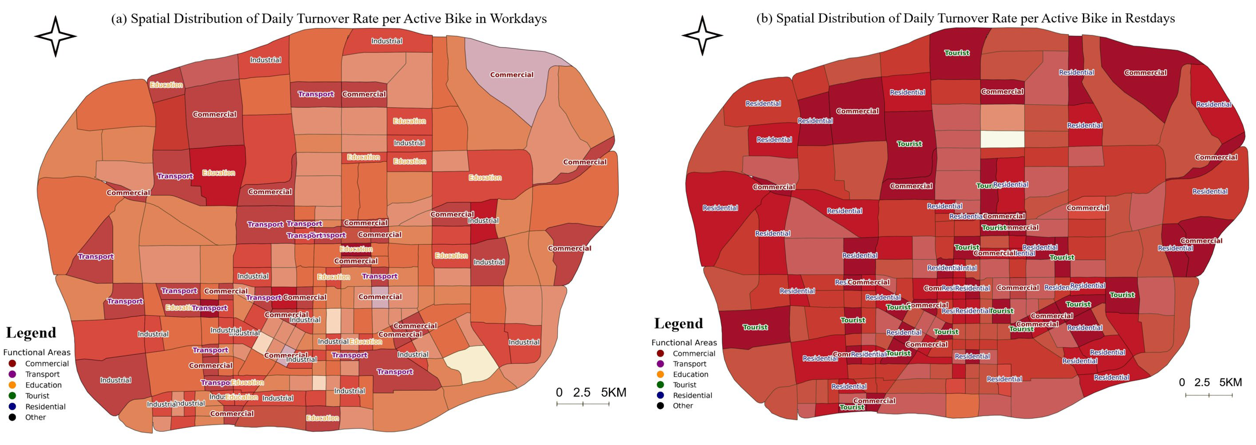
The study analyzed the spatial distribution characteristics of the Daily Turnover Rate per Active Bike in Xi’an, as shown in Figure 3. The results reveal significant spatial differentiation and clustering effects on both workdays and rest days, with clearly demarcated economic performance hotspots and coldspots that are not randomly or uniformly distributed.
On workdays, hotspots of high Daily Turnover Rate per Active Bike manifested spatial patterns closely coupled with urban commuting and business activities. These hotspots were significantly concentrated in core commercial and business office districts, such as the Bell Tower-Great South Gate area, the Gaoxin CBD, and the Xiaozhai commercial circle. Due to their dense office buildings, comprehensive commercial facilities, and large commuter flows, the turnover efficiency of bike-sharing, serving as a tool for last-mile connectivity or short-distance business trips, was extremely high in these areas. Concurrently, major transportation hubs and their radiating zones, for instance, Xi’an North Railway Station, Fangzhicheng Comprehensive Transportation Hub, and key metro interchange stations, also formed distinct high-turnover areas, where bike-sharing effectively met passengers’ last-mile connectivity needs. Furthermore, areas with high concentrations of higher education institutions (e.g., Chang’an University Town) and large-scale industrial parks (e.g., Software New Town, parts of the Economic Development Zone) also exhibited significantly high turnover rates due to the regular travel patterns of students and industrial workers.
The spatial distribution pattern of the Daily Turnover Rate per Active Bike on rest days showed a trend of diffusion and concentration towards leisure, tourism, and large residential areas, although some core commercial areas maintained their high activity levels. Traditional commercial areas like Bell Tower-Great South Gate and Xiaozhai continued to sustain very high bike turnover rates on rest days, driven by their abundant shopping, dining, and entertainment functions. More prominently, the surroundings of major tourist attractions and public recreational parks, such as the Giant Wild Goose Pagoda-Tang Paradise area, the Ming City Wall scenic route, and Qujiang Pool Park, became new turnover hotspots on rest days, clearly reflecting the activity patterns of citizens and tourists using bike-sharing for sightseeing and leisure. Simultaneously, some well-developed large residential communities, such as those in Qujiang New District and parts of the Chan-Ba Ecological District, also experienced increased bike-sharing turnover on rest days around their internal community commercial centers and lifestyle service facilities, reflecting the demand for short-distance residential trips.
Corresponding to the hotspot areas, coldspot areas of Daily Turnover Rate per Active Bike also exhibited consistent spatial distribution characteristics on both workdays and rest days. These areas were primarily located in the peripheral zones of the built-up urban area, new districts still in the early stages of development and construction (such as parts of the Xixian New Area), and zones predominantly characterized by a single residential function with relatively lagging public service facilities and transport connectivity. In these areas, the average turnover rate was significantly lower than in core urban areas and functional hotspots, owing to inherently lower travel demand density, more monolithic trip purposes, or less significant tidal effects.

4.2. Model Optimization and SHAP Factors

4.2.1. Model Training and Performance Evaluation

Subsequent to the preliminary screening and validation of variables, this study employed the XGBoost (Extreme Gradient Boosting) algorithm to construct a predictive model. The objective was to thoroughly investigate the complex impacts of various built environment variables and operational parameters on the bike-sharing economic performance index. XGBoost, a highly efficient and flexible gradient boosting decision tree algorithm, is renowned for its exceptional predictive accuracy, robust capability in capturing non-linear relationships and feature interactions, and its inherent regularization mechanisms that effectively mitigate overfitting. These attributes render it particularly suitable for analyzing the intricate and often non-linear interdependencies between the urban built environment and the economic viability of bike-sharing systems.
The model training and optimization process adhered to a rigorous machine learning workflow, aiming to develop an XGBoost model characterized by both high predictive precision and strong generalization capabilities.
Dataset Partitioning: Initially, the dataset, comprising all Transportation Analysis Zone (TAZ) samples with their corresponding features and the target economic performance index, was randomly partitioned. Eighty percent of the data was allocated to the training set, while the remaining 20% constituted an independent test set. The training set was utilized for learning model parameters and fine-tuning hyperparameters, whereas the test set served to evaluate the performance of finally selected model on unseen data.
Hyperparameter Tuning: The performance of an XGBoost model is critically dependent on its hyperparameter configuration. This study employed a comprehensive Grid Search strategy coupled with 5-fold Cross-Validation to systematically explore the parameter space. The optimization process tested extensive parameter ranges: learning_rate (0.01–0.3), max_depth (3–10), n_estimators (50–300), subsample (0.8–1.0), colsample_bytree (0.7–1.0), and regularization parameters including gamma (0–0.2), reg_alpha (0–0.1), and reg_lambda (0.1–1.0). During the cross-validation process, the primary objective was RMSE minimization while maintaining performance consistency across all validation folds (standard deviation of RMSE <5% of mean value). Following a meticulous hyperparameter optimization procedure, the finally selected optimal hyperparameter combination is shown in Table 5.
Model Performance Evaluation: The final XGBoost model was trained using the optimal hyperparameter combination identified above, and its performance was comprehensively assessed on the independent test set.
Training Data Performance: On the 80% training dataset, the XGBoost model demonstrates excellent fitting capability with R2 of 0.93, indicating the model can explain 93% of target variable variance and demonstrate strong learning capability. Training set RMSE of 10.8 represents only a slight increase compared to the test set’s 10.21, while MAE of 8.2 remains very close to the test set’s 7.89, and MSE of 116.6 shows minimal difference compared to the test set’s 104.24. The difference between training set R2 (0.93) and test set R2 (0.847) is only 8.9%, indicating excellent generalization capability without severe overfitting phenomena. Five-fold cross-validation confirmed model robustness with R2 standard deviation less than 0.02 and cross-validation average R2 of 0.89 (±0.018), highly consistent with our main results.
Figure 4 shows a scatter plot comparing the predicted economic performance index by the optimized XGBoost model against the actual observed values on the test set. The plot clearly demonstrates that the majority of data points are closely clustered around the ideal line, indicating a high degree of congruence between the model’s predictions and the actual values. Specifically, the model achieved a coefficient of determination (R2) of 0.78 on the test set, signifying its capacity to explain 78% of the variance in the economic performance index and underscoring its robust predictive power and goodness-of-fit. The presence of a few outliers suggests that specific TAZs may be influenced by idiosyncratic factors not fully captured by the model.
To further validate the superiority of the XGBoost model, Figure 5 presents a comprehensive comparative analysis of the optimized XGBoost model against a baseline linear regression model through two complementary evaluation approaches.
The bar chart component demonstrates that the XGBoost model significantly outperforms the baseline model across all evaluation metrics. Specifically, the XGBoost model achieves an R2 value of 0.847, substantially higher than the linear regression baseline model’s 0.652, representing a 30% improvement in explained variance. Concurrently, the XGBoost model exhibits considerably lower error metrics: RMSE of 10.21 compared to 15.73 (35.1% reduction), MAE of 7.89 versus 12.45 (36.6% improvement), and MSE of 104.24 against 247.43 (57.9% reduction). These consistent improvements across all performance dimensions robustly demonstrate XGBoost’s superior capability in capturing and modeling the complex non-linear relationships and feature interactions inherent in bike-sharing economic performance prediction.
The Taylor Diagram component provides a comprehensive model skill assessment that simultaneously visualizes correlation, standard deviation ratios, and centered root mean square error within a unified framework. The diagram clearly illustrates that the XGBoost model (marked point) is positioned significantly closer to the observed reference point compared to the baseline model. This proximity is evidenced by the XGBoost model exhibiting a higher correlation coefficient with the observed data (indicated by a smaller angle relative to the horizontal axis) and its standard deviation being more closely aligned with that of the observed data (demonstrated by similar radial distance from the origin). Consequently, this positioning results in a substantially smaller overall Centered Root Mean Square Error (CRMSE), indicating superior model skill in reproducing observed variability patterns.
This dual-perspective assessment—combining detailed quantitative performance metrics with comprehensive skill visualization—provides robust evidence for the superiority and reliability of the XGBoost model in predicting bike-sharing economic performance indices. The convergent results from both analytical approaches substantiate the practical value of employing advanced machine learning techniques for complex urban transportation economic modeling, particularly in scenarios involving non-linear relationships and intricate feature interactions that exceed the capabilities of traditional linear approaches.

4.2.2. Identifying Factors of Bike-Sharing Economic Performance

Through SHAP analysis, we first assessed the global importance of each input feature in predicting the bike-sharing economic performance index. As shown in Figure 6 (SHAP mean absolute value bar chart), features are ranked according to their average absolute impact on the model’s output. The results clearly indicate that Bike Supply Density is the most influential factor, possessing the highest mean absolute SHAP value. Following this, Commercial POI Density, Proximity to Public Transit (m), and Residential Density collectively constitute the core drivers impacting bike-sharing economic performance. While Road Network Density and Average Income also contribute to the model, their global importance is relatively lower.
To gain a more nuanced understanding of the direction and distribution of each feature’s impact, Figure 6 presents the SHAP summary plot (beeswarm plot). In this plot, each point represents a TAZ sample; its color denotes the original value of the feature (red for high values, blue for low values), and its horizontal position indicates the SHAP value (positive or negative impact) of that feature for the respective sample’s prediction. Observations from Figure 6b include:
Points for Bike Supply Density are predominantly distributed in the positive SHAP value region, and as the color transitions from blue to red (i.e., feature value increases), the SHAP values tend to increase. This suggests that, overall, increasing bike supply density enhances the economic performance index, although the distribution also highlights the complexity of this effect.
High values (red points) for Commercial POI Density and Average Income also generally correspond to positive SHAP values, indicating that an increase in these factors contributes to improved economic performance.
Points for Proximity to Public Transit (m) exhibit an inverse trend: high values (red points, indicating a greater distance to transit stops) mainly correspond to negative SHAP values, whereas low values (blue points, indicating proximity to transit stops) are associated with more positive SHAP values. This aligns with the intuitive understanding that better proximity to public transit (shorter distance) is conducive to higher economic performance.

4.3. Non-Linear Effects, Interactions, and Individual Explanations

4.3.1. Non-Linear Effects and Primary Interactions

SHAP Dependence Plots are crucial tools for revealing how a single feature non-linearly impacts the model’s predictions and how this impact is modulated by another feature. The following details the interpretation of SHAP dependence plots for six core features, as shown in Figure 7a–f.
Non-linear Impact of Bike Supply Density (Interaction Feature: Commercial POI Density) As shown in Figure 7a, Bike Supply Density exhibits a gradual positive trend in SHAP values for the economic performance index. At low supply densities (0–10 bikes/km2), SHAP values remain near zero. As density increases from approximately 10 bikes/km2 to 40 bikes/km2, SHAP values show progressive increase, reaching a maximum of approximately +1.0. The relationship demonstrates consistent positive contribution rather than dramatic threshold effects, indicating that bike supply density provides steady but moderate benefits to economic performance.
The color coding in the plot represents Commercial POI Density rather than Proximity to Public Transit as initially stated. It is observable that, at equivalent levels of Bike Supply Density (e.g., 30 bikes/km2), points Diabetes Mellitus with a lighter color (indicating closer proximity to transit stations, e.g., <200 m) systematically exhibit higher SHAP values than darker points (indicating greater distance from transit stations, e.g., >800 m). This signifies that excellent public transit connectivity (shorter distances) amplifies the positive economic effects of bike supply.
Non-linear Impact of Commercial POI Density (Interaction Feature: Bike Supply Density) Figure 7b demonstrates that Commercial POI Density shows a positive relationship with SHAP values, though the pattern exhibits considerable scatter. The relationship suggests generally positive contributions across the range of commercial densities, with SHAP values ranging from approximately −0.5 to +1.5, but without clear threshold effects or dramatic non-linear patterns. The color encoding represents Bike Supply Density, indicating that areas with higher bike supply (darker points) tend to achieve higher SHAP values for commercial POI density, supporting the synergistic relationship between commercial activity and bike availability.
Non-linear Impact of Residential Density (Interaction Feature: Bike Supply Density) As shown in Figure 7c, Residential Density shows scattered oscillation around zero across its range, with SHAP values primarily distributed between −0.5 and +0.5. The pattern does not exhibit the clear inverted U-shape initially suggested, but rather shows complex variability that may reflect the diverse roles of residential areas in bike-sharing usage patterns depending on local context and supporting infrastructure. The point color (and the right-hand vertical axis) represents Bike Supply Density. In areas with moderate residential density, a higher bike supply density (darker points) often corresponds to higher SHAP values, suggesting that an increased bike supply effectively enhances economic benefits in areas with a stable residential population.
Non-linear Impact of Proximity to Public Transit (m) (Interaction Feature: Bike Supply Density) Figure 7d shows that proximity to public transit (where smaller distances indicate closer proximity) generally exhibits positive SHAP values when TAZs are close to transit stations, with values ranging from approximately +0.25 to −0.3 across the distance spectrum. The relationship suggests that closer proximity to transit generally supports better economic performance, though the effect magnitude is more moderate than initially described. The point color (and the right-hand vertical axis) represents Bike Supply Density. In areas with good proximity to public transit (shorter distance), a higher bike supply density (darker points) will result in larger positive SHAP values. Conversely, in areas poorly served by public transit, even an increase in bike supply may have a limited positive impact on its SHAP value, struggling to counteract the negative effects of transit inconvenience.
Non-linear Impact of Road Network Density (km/km2) (Interaction Feature: Bike Supply Density) Figure 7e demonstrates that Road Network Density shows minimal variation in SHAP values near zero across its range, suggesting limited impact on economic performance. The relationship appears relatively flat, indicating that road network density may not be a primary driver of bike-sharing economic performance within the studied range. The point color (and the right-hand vertical axis) signifies Bike Supply Density. In areas with higher road network density, coupled with a higher bike supply density (darker points), the SHAP value will be higher, suggesting that good road accessibility is fundamental for efficient bike circulation and, when combined with adequate supply, can better realize benefits.
Non-linear Impact of Average Income (Yuan) (Interaction Feature: Bike Supply Density) Figure 7f indicates a generally monotonic positive relationship between Average Income and SHAP values, without clear non-monotonic patterns. The relationship shows steady increase rather than the complex inverted pattern initially described, suggesting that higher income areas consistently support better bike-sharing economic performance. The point color (and the right-hand vertical axis) indicates Bike Supply Density. In areas with moderate income levels and higher bike supply density (darker points), the positive contribution of the income factor might be amplified.

4.3.2. Interaction Effects Among Features

Understanding these interaction patterns provides critical insights for urban policy and operational decision-making. The SHAP interaction analysis reveals that bike-sharing economic optimization requires integrated strategies that consider synergistic relationships rather than isolated interventions.
Interaction effects among features are pivotal for understanding complex system behaviors. The SHAP Interaction Heatmap (SHAP Heatmap Plot for Feature Interactions, as shown in Figure 8, provides an intuitive and quantitative overview of the average absolute SHAP interaction effect strength between pairs of features in the model. In the heatmap, the intensity of the cell color (or the directly annotated numerical value) represents the extent to which the combined effect of two features on the model’s prediction deviates from the sum of their individual independent effects. Stronger interaction effects imply that the combined configuration of these two factors has a greater non-linear influence on the final outcome. From the heatmap, we can meticulously interpret the following interaction patterns:
(1) Dominant Interactions: Strong Synergies between Bike Supply Density and Core Built Environment Elements
Bike Supply Density and Commercial POI Density: This pair typically exhibits one of the strongest positive interaction effects. For instance, their average absolute SHAP interaction value might be as high as 1.5–2.0. This signifies that in areas with high concentrations of commercial activity (high Commercial POI Density), increasing the bike supply (enhancing Bike Supply Density) leads to a far greater improvement in economic performance than increasing the bike supply by the same amount in areas with sparse commercial activity. Conversely, if a high Commercial POI Density area has insufficient bike supply, its locational advantages cannot be fully translated into economic benefits for bike-sharing. This strong synergy suggests that operators should prioritize optimizing bike deployment in high commercial density zones to create hotspots in order to get a hotter effect.
Bike Supply Density and Proximity to Public Transit: A significant positive interaction also exists between these two, with an interaction strength potentially second only to the former (e.g., average absolute SHAP interaction values between 1.2 and 1.7). This implies that in areas close to transit stations (high Proximity to Public Transit), a moderate increase in bike supply can more effectively enhance last-mile connectivity efficiency and vehicle turnover rates. In contrast, in areas far from transit stations, even a substantial bike supply might have limited positive impact on economic performance. This provides a quantitative basis for transit hub + bike synergistic deployment strategies.
(2) Important Interactions: Mutual Reinforcement among Built Environment Elements
Commercial POI Density and Proximity to Public Transit: These two core-built environment elements usually also demonstrate a relatively strong positive interaction (e.g., interaction values between 0.8 and 1.3). An area that is both a commercial center and possesses convenient public transportation will generate significantly higher demand and usage frequency for bike-sharing compared to areas with only one of these advantages. This interaction underscores the importance of integrating mixed land use and transport accessibility in urban planning.
Bike Supply Density and Residential Density: The strength of this interaction might be moderate (e.g., 0.6–1.1). In areas with a certain residential population base (medium to high Residential Density), a reasonable bike supply can better meet residents’ daily travel needs, thereby enhancing economic performance. However, in areas with excessively high residential density but inadequate supporting facilities (such as commercial or transport), the interaction effect of simply increasing bike supply might be less pronounced.
Bike Supply Density and Road Network Density: Although intuitively, road network density is crucial for bike operations, its interaction strength with bike supply might be less potent than the combinations mentioned above, or its interaction effect might saturate after road network density reaches a certain threshold. A good road network is fundamental, but its multiplicative effect with supply quantity might be more evident within specific ranges.
Interactions involving Average Income: The interaction effects of the income factor can be more complex and nuanced. For example, in middle-income, high-commercial-density areas, the interaction effect of increasing bike supply might be stronger than in low-income or extremely high-income areas with similar commercial characteristics. This requires interpretation in conjunction with specific dependence plots.
(3) Practical Implications from Interaction Effects
When deploying or rebalancing bikes, decisions should not be based solely on the level of a single factor. Instead, priority should be given to golden zones where key factors are favorably combined (e.g., high Commercial POI Density + high Proximity to Public Transit + moderately high Bike Supply Density). This targeted approach can yield disproportionately higher returns on investment.
Urban planning departments, during new area development or old district regeneration, should consider how to create a more conducive operational environment for green transport modes like bike-sharing by optimizing built environment elements (e.g., enhancing commercial clustering, improving public transit services, densifying road networks). Such integrated planning can amplify the positive externalities of bike-sharing systems.
Operators can leverage their understanding of interaction effects to dynamically adjust strategies in different urban functional zones and at different times, based on real-time changes in built environment characteristics (e.g., temporary commercial events, fluctuations in passenger flow at transport hubs). For instance, during large-scale events in commercial districts, significantly increasing bike supply in the short term can yield marginal benefits far exceeding those during normal periods due to heightened interaction effects. This allows for agile and responsive management that maximizes both economic efficiency and social utility.
By pinpointing the strongest positive interactions, cities can identify the most effective leverage points for interventions. For example, if the interaction between bike supply and transit proximity is particularly strong, investments in improving bike parking and access at transit stations could yield substantial benefits for the bike-sharing ecosystem.
Conversely, understanding weaker or negative interactions can help avoid suboptimal investments. If simply increasing bike supply in low-density residential areas with poor transit access shows weak interaction effects, resources might be better allocated elsewhere until the complementary infrastructure or density improves.
By quantitatively analyzing these interaction effects, we can move beyond linear thinking and single-factor decision-making, guiding the sustainable development of bike-sharing systems more scientifically.

4.3.3. Attribution Analysis of Individual TAZ Predictions

Another core value of SHAP analysis lies in its capability for fine-grained attribution of the model’s specific predictions for each sample (in this case, TAZ1). This is achieved through SHAP Waterfall Plots.
Figure 9 shows the SHAP waterfall plot for the economic performance index prediction of TAZ1. The model’s final predicted economic performance index for TAZ1 is f(x) = 0.612. This predicted value is derived by starting from the model’s base value, E[f(x)] (i.e., the average predicted economic performance index across all training samples), and then summing the SHAP values of each feature for TAZ1. Based on the provided data, the sum of SHAP contributions for the features is 0.78 − 0.23 + 0.10 − 0.06 + 0.05 + 0.02 = 0.66. Therefore, the model’s base value E[f(x)] can be calculated as 0.612 − 0.66 = −0.048. (Note: A negative base value might indicate that the economic performance index itself has been standardized or has a specific definition leading to a negative average, or it could be due to the characteristics of the data distribution.) For TAZ1, the actual values of its features and their contributions (SHAP values) to the prediction are as follows:
Bike Supply Density: Actual value = 15.747 (units: bikes/km2). Its SHAP value contribution is +0.78 (red bar). This indicates that the bike supply density in TAZ1 is the most significant positive driver of its predicted economic performance, contributing far more than the model’s average expectation for this feature.
Proximity to Transit: Actual value = 1.903 (units: meters). Its SHAP value is −0.23 (blue bar). This is a particularly noteworthy finding. Despite the extremely close proximity to a transit stop (1.903 m is practically at the stop), this feature value contributes negatively to the economic performance index in the specific context of TAZ1. This could suggest the presence of adverse micro-environmental factors around this specific transit stop (e.g., poor connectivity for bikes, unsafe or unpleasant station environment, physical barriers for bike access), or it might indicate that the model has learned a complex non-linear relationship or an interaction with other unmodeled factors at this extreme low-value range for proximity. This anomaly warrants further on-site investigation.
Average Income: Actual value = 15,671.378 (units: Yuan). Its SHAP value is +0.10 (red bar). This signifies that the average income level in TAZ1 provides a moderate positive contribution to its economic performance index. Road Network Density: Actual value = 8.319 (units: km/km2). Its SHAP value is −0.06 (blue bar). In this instance, the road network density of TAZ1 slightly detracts from its predicted economic performance, possibly indicating that its density is relatively insufficient or its structure is not optimal for bike travel.
Commercial POI Density: Actual value = 3.924 (units: POIs/km2). Its SHAP value is +0.05 (red bar). The Commercial POI density in TAZ1 is relatively low, yet it still offers a slight positive contribution, implying that even a minimal commercial presence holds some value. Residential Density: Actual value = 4.077 (units: thousands persons/km2, assumed). Its SHAP value is +0.02 (red bar). The residential density of TAZ1 also makes a very small positive contribution. Summing the base value and all feature SHAP values: −0.048 + 0.78 − 0.23 + 0.10 − 0.06 + 0.05 + 0.02 = 0.612, which precisely matches the model’s final prediction for TAZ1.
This type of individual-level attribution analysis enables decision-makers not only to know the model’s prediction but also to clearly understand how this result is shaped by the interplay of various specific factors. For TAZ1, its high bike supply density is a major strength. However, the counterintuitive negative impact of extremely close transit proximity flags a critical area for detailed local assessment. The road network density also appears as a potential, albeit minor, area for improvement. Such fine-grained diagnostics provide a robust scientific basis for formulating site-specific optimization strategies for bike-sharing systems.

5. Discussion

5.1. Spatial Heterogeneity and Threshold Effects in Bike-Sharing Economic Performance

The economic performance and sustainable operation of bike-sharing systems are critical research foci within the broader context of urban sustainable transportation. While existing studies have identified various influencing factors, there remains limited evidence on the complex non-linear mechanisms, particularly threshold effects and intricate interaction effects, governing the relationship between network operational characteristics, built environment features, and economic outcomes. This study, grounded in Xi’an, China, employed an integrated methodological framework encompassing spatial analysis techniques, advanced machine learning (XGBoost), and robust interpretability methods (SHAP).
Our findings regarding spatial heterogeneity in bike-sharing economic performance align with but extend beyond previous studies that primarily focused on usage patterns rather than economic optimization. Former studies have consistently demonstrated that bike-sharing activity clusters in central business districts and areas with high population density. Our research confirms this general pattern for economic performance in Xi’an but adds a crucial layer of nuance through the identification of nonlinearities. Unlike studies which used Random Forest for demand prediction and found predominantly linear relationships, our XGBoost–SHAP approach reveals distinct threshold effects [63]. The economic performance of bike-sharing exhibits significant spatial heterogeneity intricately coupled with the city’s urban functional structure, a pattern largely driven by the combined influence of localized demand, operational factors, and specific built environment compositions as revealed by interpretable machine learning. Areas exhibiting high economic performance are predominantly concentrated in zones with specific functional attributes (e.g., high commercial activity, proximity to transit hubs) and high levels of urban activity, as quantitatively confirmed by their strong positive SHAP contributions.
Our discovery of threshold effects challenges the simplistic ‘more is better’ assumption often implicit in linear models used in earlier bike-sharing research, as seen in some early planning models. For example, we identified that beyond a certain density of commercial POIs, the marginal economic return begins to diminish. This finding provides a critical counterpoint to studies that only report a positive linear correlation between commercial density and ridership [64]. The existence of such thresholds suggests that in hyper-concentrated commercial zones, the market may become saturated, or competition from other transport modes (like walking or subways for very short trips) becomes more intense. This non-linear insight is vital for optimizing resource allocation, preventing wasteful over-supply in already saturated areas.
While our SHAP analysis reveals strong associational patterns between various factors and economic performance, it is crucial to emphasize that these findings represent associations rather than causal relationships. The threshold effects identified should be interpreted as empirical patterns requiring theoretical validation and careful consideration of potential confounding factors. Interestingly, the threshold for bike supply density in our study was less pronounced than for built environment factors. This contrasts with studies from some European cities that reported sharper saturation points for fleet size [65]. This difference could be attributed to Xi’an’s higher population density and a still-growing cycling culture, suggesting that the system may not have reached its absolute capacity limits, unlike more mature systems. This highlights how operational thresholds are context-dependent, shaped by both urban form and local mobility behaviors.

5.2. Interaction Effects and Operational Complexity

Complex interaction effects exist among the various influencing factors, where the economic performance is a multiplicative outcome of their strategic interplay rather than a simple sum, highlighting the necessity of synergistic optimization strategies. This moves significantly beyond the scope of many prior studies that analyzed influencing factors in isolation [66]. Our work empirically demonstrates the synergistic principle that the whole is greater than the sum of its parts in bike-sharing systems. The study elucidated, through SHAP interaction heatmaps and dependence plots, that the impact of any single factor on economic performance is not isolated but is significantly moderated and conditioned by other concurrent factors. For instance, the positive effect of optimizing bike supply density is substantially amplified in areas with a supportive built environment, such as high Commercial POI Density or excellent Proximity to Public Transit. This specific interaction finding provides quantitative evidence for the long-held planning concept of ‘transit-oriented development’ (TOD) in the context of bike-sharing economics. While research has qualitatively argued for integrating bike-sharing with public transit [67], our study provides specific, data-driven evidence of the amplified economic returns, showing that bikes are most profitable when they serve as first-and-last-mile connectors in commercially vibrant, transit-rich environments.
The interaction effects identified in our study must be understood within Xi’an’s specific governance context, characterized by public–private partnerships and municipal regulatory oversight. Different operator structures (purely private vs. subsidized systems) may exhibit varying threshold behaviors and interaction patterns. For instance, subsidized systems might demonstrate different optimal density thresholds compared to market-driven operations, as financial constraints and user fee structures significantly influence demand patterns and operational viability. Municipal policies regarding bike parking regulations, integration with public transit systems, and area access restrictions also serve as crucial moderating factors that can amplify or diminish the interaction effects we identified.
Our current analysis, while comprehensive in scope, acknowledges significant limitations in capturing qualitative aspects of cycling infrastructure. Simple road density metrics cannot adequately represent crucial factors such as dedicated bike lane continuity and protection levels, intersection safety features, street lighting adequacy, and pedestrian-cyclist conflict zones. These infrastructure quality dimensions directly influence user safety perceptions and willingness to use shared bikes, potentially serving as critical moderators of the threshold effects we identified.

5.3. Methodological Contributions and Policy Implications

The analytical framework adopted in this study, integrating machine learning with advanced interpretability techniques like SHAP, provides a robust and transparent approach for dissecting non-linear relationships and interaction effects within complex urban systems. This offers valuable methodological insights for future research in urban science, transport planning, and the sharing economy, moving beyond “black-box” models to actionable intelligence. By demonstrating how to extract specific thresholds and interaction effects, our work provides a tangible bridge between the predictive power of machine learning and the explanatory needs of urban planners, a gap often highlighted in the literature [68].
While our analytical framework demonstrates robust performance within Xi’an’s context, the transferability of specific findings to other urban environments requires careful consideration. Cities with different urban morphologies, varying climate conditions, distinct cycling cultures, and alternative governance structures may exhibit substantially different threshold patterns and interaction effects. The methodological approach—integrating XGBoost with SHAP for threshold identification—appears broadly applicable, but the specific threshold values and interaction magnitudes identified in Xi’an should not be directly applied elsewhere without local calibration and validation.
For practitioners, the findings support development of spatially differentiated operational strategies based on local urban characteristics and interaction patterns. The identification of synergistic effects between bike supply density and commercial activity concentration provides evidence for targeted deployment strategies in high-potential areas. Urban planners can leverage these insights to create more supportive environments for shared mobility through integrated land use and transportation planning, particularly in developing mixed-use areas with strong transit connectivity. The interaction patterns identified suggest that bike-sharing optimization requires integrated approaches that transcend single-factor decision-making. For operators, this implies dynamic management strategies that consider local context variations and factor synergies. For municipal authorities, the findings support policies that facilitate operator-transit authority coordination and integrated infrastructure development to maximize system-wide benefits.

5.4. Research Limitations and Future Directions

While the evaluation metrics employed in this study (R2, RMSE, MAE, MSE) are widely used in machine learning and transportation research with good comparability, comprehensive indicators such as Performance Index (PI) and Nash-Sutcliffe efficiency (NSE) could provide more holistic perspectives on model performance evaluation [69]. These advanced metrics, which combine multiple performance dimensions including bias, correlation, and variability measures, would enhance the robustness of model validation and enable more nuanced understanding of prediction reliability across different operational conditions.
The one-month data period, while avoiding major holidays and capturing typical spring operational patterns, may not fully represent annual usage patterns due to seasonal variations in weather, tourism, and user behavior. This temporal constraint, combined with the hypothetical nature of some variables, necessitates cautious interpretation of findings, particularly regarding the stability of identified threshold effects across different seasons and years. The single-city focus, while enabling deep contextual analysis, limits direct generalizability and highlights the need for multi-city comparative studies to validate the broader applicability of our methodological framework.
Future research should aim to incorporate longer-term dynamic analyses considering factors like seasonality and evolving urban landscapes, a more comprehensive assessment of multi-dimensional economic, social, and environmental impacts, and a deeper exploration of user behavior heterogeneity and its underlying socio-demographic drivers. Priority areas for future investigation include longitudinal studies spanning multiple seasons and years to validate threshold stability and seasonal variation patterns; multi-city comparative analyses to test framework transferability across different urban contexts; integration of real-time operational data, weather conditions, and detailed infrastructure quality metrics; incorporation of causal inference techniques to move beyond associational relationships toward causal understanding; and development of dynamic optimization models that can adapt to changing urban conditions and policy interventions. This continued investigation will contribute to the development of more resilient, equitable, and efficient urban mobility solutions, fostering the sustainable integration of bike-sharing into the fabric of modern cities.

6. Conclusions

This study provides comprehensive insights into the complex relationships governing bike-sharing economic performance through an innovative integration of spatial analysis, machine learning, and interpretability techniques. The research yields several key contributions to urban transportation and mobility planning literature while acknowledging important limitations that inform future research directions.
Our analysis reveals three fundamental insights into bike-sharing economic optimization. First, bike-sharing economic performance exhibits pronounced spatial heterogeneity closely aligned with urban functional structure, with high-performing areas concentrated in zones featuring commercial activity and transit accessibility. Second, various factors demonstrate positive but moderate relationships with economic performance, characterized by gradual trends rather than dramatic threshold effects, with bike supply density showing consistent positive contributions and interaction effects playing important moderating roles. Third, complex interaction effects exist among influencing factors, with economic performance representing multiplicative outcomes of strategic factor interplay rather than simple additive relationships.
Theoretically, this research advances understanding of complex relationships in urban mobility systems while emphasizing the associational rather than causal nature of identified patterns. The identification of moderate non-linear relationships and interaction effects challenges traditional linear modeling approaches and supports more sophisticated analytical frameworks. Methodologically, the integration of XGBoost with SHAP analysis provides a powerful approach for combining predictive accuracy with interpretability, addressing the persistent challenge of “black-box” machine learning in policy-relevant research.
For practitioners, the findings support development of spatially differentiated operational strategies based on local urban characteristics and interaction patterns. The identification of synergistic effects between bike supply density and commercial activity concentration provides evidence for targeted deployment strategies in high-potential areas. Urban planners can leverage these insights to create more supportive environments for shared mobility through integrated land use and transportation planning, particularly in developing mixed-use areas with strong transit connectivity. The interaction patterns identified suggest that bike-sharing optimization requires integrated approaches that transcend single-factor decision-making. For operators, this implies dynamic management strategies that consider local context variations and factor synergies. For municipal authorities, the findings support policies that facilitate operator-transit authority coordination and integrated infrastructure development to maximize system-wide benefits.
Several limitations warrant acknowledgment for proper interpretation of findings. The hypothetical nature of some variables may constrain generalization beyond Xi’an’s specific context, while the one-month data period limits understanding of seasonal variation patterns. The current evaluation framework, while robust, could benefit from incorporating advanced metrics such as Performance Index (PI) and Nash-Sutcliffe efficiency (NSE) to provide more comprehensive model validation. Priority areas for future investigation include longitudinal studies spanning multiple seasons and years to validate threshold stability and seasonal variation patterns; multi-city comparative analyses to test framework transferability across different urban contexts; integration of real-time operational data, weather conditions, and detailed infrastructure quality metrics; incorporation of causal inference techniques to move beyond associational relationships toward causal understanding; and development of dynamic optimization models that can adapt to changing urban conditions and policy interventions.
This research contributes to the broader goal of developing evidence-based approaches to sustainable urban mobility planning. The methodological framework developed here demonstrates how advanced analytical techniques can bridge the gap between complex urban data and actionable policy insights. As cities worldwide grapple with transportation sustainability challenges, the integration of machine learning with interpretability tools provides a pathway for developing more effective, context-sensitive mobility solutions. The findings challenge simplistic assumptions about urban mobility optimization while providing concrete guidance for policy and operational decision-making. While results are specific to Xi’an’s urban context, the analytical framework offers broader applicability for similar urban environments, contributing to the advancement of data-driven approaches in sustainable urban mobility planning. As bike-sharing systems continue to evolve as integral components of urban transportation networks, the evidence-based approaches demonstrated in this study provide essential tools for achieving economically viable and environmentally sustainable mobility solutions.

Author Contributions

Conceptualization, Haolong Yang and Chao Gao; methodology, Haolong Yang and Chao Gao; software, Haolong Yang; validation, Chao Gao, and Chen Feng; resources, Chen Feng; data curation, Haolong Yang; writing—original draft preparation, Haolong Yang and Chao Gao; writing—review and editing, Chen Feng; visualization, Chao Gao; supervision, Chen Feng; project administration, Chen Feng; funding acquisition, Chen Feng. All authors have read and agreed to the published version of the manuscript.

Funding

This research was funded in part by the National Natural Science Foundation of China under Grant 72303176, the Postdoctoral Science Foundation of China under Grant 2024T170709, the Shaanxi Provincial Youth Science and Technology Star Talent Program under Grant, 2025ZC-KJXX-18 and the Xi’an Social Science Planning Fund Project under Grant 25GL124.

Data Availability Statement

Data will be made available on request.

Conflicts of Interest

The authors declare no conflicts of interest.

References

  1. Albuquerque, V.; Sales Dias, M.; Bacao, F. Machine Learning Approaches to Bike-Sharing Systems: A Systematic Literature Review. ISPRS Int. J. Geo-Inf. 2021, 10, 62. [Google Scholar] [CrossRef]
  2. Zhang, L.; Zhang, J.; Duan, Z.; Bryde, D. Sustainable Bike-Sharing Systems: Characteristics and Commonalities across Cases in Urban China. J. Clean. Prod. 2015, 97, 124–133. [Google Scholar] [CrossRef]
  3. Oostendorp, R.; Gebhardt, L. Combining Means of Transport as a Users’ Strategy to Optimize Traveling in an Urban Context: Empirical Results on Intermodal Travel Behavior from a Survey in Berlin. J. Transp. Geogr. 2018, 71, 72–83. [Google Scholar] [CrossRef]
  4. Cai, J.; Zheng, P.; Xie, Y.; Du, Z.; Li, X. Research on the Impact of Climate Change on Green and Low-Carbon Development in Agriculture. Ecol. Indic. 2025, 170, 113090. [Google Scholar] [CrossRef]
  5. Ma, Y.; Rong, K.; Mangalagiu, D.; Thornton, T.F.; Zhu, D. Co-Evolution between Urban Sustainability and Business Ecosystem Innovation: Evidence from the Sharing Mobility Sector in Shanghai. J. Clean. Prod. 2018, 188, 942–953. [Google Scholar] [CrossRef]
  6. Mooney, S.J.; Hosford, K.; Howe, B.; Yan, A.; Winters, M.; Bassok, A.; Hirsch, J.A. Freedom from the Station: Spatial Equity in Access to Dockless Bike Share. J. Transp. Geogr. 2019, 74, 91–96. [Google Scholar] [CrossRef]
  7. Qiu, L.-Y.; He, L.-Y. Bike Sharing and the Economy, the Environment, and Health-Related Externalities. Sustainability 2018, 10, 1145. [Google Scholar] [CrossRef]
  8. Nikitas, A. How to Save Bike-Sharing: An Evidence-Based Survival Toolkit for Policy-Makers and Mobility Providers. Sustainability 2019, 11, 3206. [Google Scholar] [CrossRef]
  9. Eren, E.; Uz, V.E. A Review on Bike-Sharing: The Factors Affecting Bike-Sharing Demand. Sustain. Cities Soc. 2020, 54, 101882. [Google Scholar] [CrossRef]
  10. Li, Z.; Wang, W.; Yang, C.; Ding, H. Bicycle Mode Share in China: A City-Level Analysis of Long Term Trends. Transportation 2017, 44, 773–788. [Google Scholar] [CrossRef]
  11. Hu, S.; Xiong, C.; Liu, Z.; Zhang, L. Examining Spatiotemporal Changing Patterns of Bike-Sharing Usage during COVID-19 Pandemic. J. Transp. Geogr. 2021, 91, 102997. [Google Scholar] [CrossRef]
  12. Chen, Q.; Fu, C.; Zhu, N.; Ma, S.; He, Q.-C. A Target-Based Optimization Model for Bike-Sharing Systems: From the Perspective of Service Efficiency and Equity. Transp. Res. Part B Methodol. 2023, 167, 235–260. [Google Scholar] [CrossRef]
  13. Saltykova, K.; Ma, X.; Yao, L.; Kong, H. Environmental Impact Assessment of Bike-Sharing Considering the Modal Shift from Public Transit. Transp. Res. Part Transp. Environ. 2022, 105, 103238. [Google Scholar] [CrossRef]
  14. Lin, L.; He, Z.; Peeta, S. Predicting Station-Level Hourly Demand in a Large-Scale Bike-Sharing Network: A Graph Convolutional Neural Network Approach. Transp. Res. Part C Emerg. Technol. 2018, 97, 258–276. [Google Scholar] [CrossRef]
  15. Jing, Y.; Sun, R.; Chen, L. A Method for Identifying Urban Functional Zones Based on Landscape Types and Human Activities. Sustainability 2022, 14, 4130. [Google Scholar] [CrossRef]
  16. Sugiarto, H.; Yanti, J.; Cahyani, D.; Junaidi, A.; Oktoriza, L.A. Exploration Financial Performance Optimization Strategies on Business Success: A Literature Review. SEIKO J. Manag. Bus. 2023, 6, 402–411. Available online: https://www.repository.unimas.ac.id/index.php?p=show_detail&id=335&keywords= (accessed on 25 August 2025).
  17. Siqueira-Gay, J.; Giannotti, M.; Sester, M. Learning about Spatial Inequalities: Capturing the Heterogeneity in the Urban Environment. J. Clean. Prod. 2019, 237, 117732. [Google Scholar] [CrossRef]
  18. Zhang, J.; Cheng, L. Threshold Effect of Tourism Development on Economic Growth Following a Disaster Shock: Evidence from the Wenchuan Earthquake, PR China. Sustainability 2019, 11, 371. [Google Scholar] [CrossRef]
  19. Chen, E.; Ye, Z. Identifying the Nonlinear Relationship between Free-Floating Bike Sharing Usage and Built Environment. J. Clean. Prod. 2021, 280, 124281. [Google Scholar] [CrossRef]
  20. Mavlutova, I.; Atstaja, D.; Grasis, J.; Kuzmina, J.; Uvarova, I.; Roga, D. Urban Transportation Concept and Sustainable Urban Mobility in Smart Cities: A Review. Energies 2023, 16, 3585. [Google Scholar] [CrossRef]
  21. Zhao, Q.; Jiang, M.; Zhao, Z.; Liu, F.; Zhou, L. The Impact of Green Innovation on Carbon Reduction Efficiency in China: Evidence from Machine Learning Validation. Energy Econ. 2024, 133, 107525. [Google Scholar] [CrossRef]
  22. Ustaoglu, F.; Islam, M.S. Potential Toxic Elements in Sediment of Some Rivers at Giresun, Northeast Turkey: A Preliminary Assessment for Ecotoxicological Status and Health Risk. Ecol. Indic. 2020, 113, 106237. [Google Scholar] [CrossRef]
  23. Gao, K.; Yang, Y.; Gil, J.; Qu, X. Data-Driven Interpretation on Interactive and Nonlinear Effects of the Correlated Built Environment on Shared Mobility. J. Transp. Geogr. 2023, 110, 103604. [Google Scholar] [CrossRef]
  24. Chikaraishi, M.; Garg, P.; Varghese, V.; Yoshizoe, K.; Urata, J.; Shiomi, Y.; Watanabe, R. On the Possibility of Short-Term Traffic Prediction during Disaster with Machine Learning Approaches: An Exploratory Analysis. Transp. Policy 2020, 98, 91–104. [Google Scholar] [CrossRef]
  25. Yang, C.; Chen, M.; Yuan, Q. The Application of XGBoost and SHAP to Examining the Factors in Freight Truck-Related Crashes: An Exploratory Analysis. Accid. Anal. Prev. 2021, 158, 106153. [Google Scholar] [CrossRef]
  26. Wang, L.; Zhao, C.; Liu, X.; Chen, X.; Li, C.; Wang, T.; Wu, J.; Zhang, Y. Non-Linear Effects of the Built Environment and Social Environment on Bus Use among Older Adults in China: An Application of the XGBoost Model. Int. J. Environ. Res. Public. Health 2021, 18, 9592. [Google Scholar] [CrossRef]
  27. Jiang, J.; Li, Y.; Li, Y.; Li, C.; Yu, L.; Li, L. Smart Transportation Systems Using Learning Method for Urban Mobility and Management in Modern Cities. Sustain. Cities Soc. 2024, 108, 105428. [Google Scholar] [CrossRef]
  28. Wu, P.; Zhang, Z.; Peng, X.; Wang, R. Deep Learning Solutions for Smart City Challenges in Urban Development. Sci. Rep. 2024, 14, 5176. [Google Scholar] [CrossRef]
  29. Shen, H.; Weng, J.; Lin, P. Exploring the Nuanced Correlation between Built Environment and the Integrated Travel of Dockless Bike-Sharing and Metro at Origin-Route-Destination Level. Sustain. Cities Soc. 2025, 119, 106090. [Google Scholar] [CrossRef]
  30. Lai, X.; Gao, C. Spatiotemporal Patterns Evolution of Residential Areas and Transportation Facilities Based on Multi-Source Data: A Case Study of Xi’an, China. ISPRS Int. J. Geo-Inf. 2023, 12, 233. [Google Scholar] [CrossRef]
  31. Zhang, X.; Wang, J.; Long, X.; Li, W. Understanding the Intention to Use Bike-Sharing System: A Case Study in Xi’an, China. PLoS ONE 2021, 16, e0258790. [Google Scholar] [CrossRef]
  32. Gao, K.; Yang, Y.; Li, A.; Li, J.; Yu, B. Quantifying Economic Benefits from Free-Floating Bike-Sharing Systems: A Trip-Level Inference Approach and City-Scale Analysis. Transp. Res. Part Policy Pract. 2021, 144, 89–103. [Google Scholar] [CrossRef]
  33. Robinson, J. Cities in a World of Cities: The Comparative Gesture. Int. J. Urban Reg. Res. 2010, 35, 1–23. [Google Scholar] [CrossRef]
  34. Zhang, F.; Liu, W. An Economic Analysis of Integrating Bike Sharing Service with Metro Systems. Transp. Res. Part Transp. Environ. 2021, 99, 103008. [Google Scholar] [CrossRef]
  35. Storme, T.; Casier, C.; Azadi, H.; Witlox, F. Impact Assessments of New Mobility Services: A Critical Review. Sustainability 2021, 13, 3074. [Google Scholar] [CrossRef]
  36. Standing, C.; Standing, S.; Biermann, S. The Implications of the Sharing Economy for Transport. Transp. Rev. 2019, 39, 226–242. [Google Scholar] [CrossRef]
  37. Ricci, M. Bike Sharing: A Review of Evidence on Impacts and Processes of Implementation and Operation. Res. Transp. Bus. Manag. 2015, 15, 28–38. [Google Scholar] [CrossRef]
  38. Lan, J.; Ma, Y.; Zhu, D.; Mangalagiu, D.; Thornton, T.F. Enabling Value Co-Creation in the Sharing Economy: The Case of Mobike. Sustainability 2017, 9, 1504. [Google Scholar] [CrossRef]
  39. Gong, Y.; Palmer, S.; Gallacher, J.; Marsden, T.; Fone, D. A Systematic Review of the Relationship between Objective Measurements of the Urban Environment and Psychological Distress. Environ. Int. 2016, 96, 48–57. [Google Scholar] [CrossRef]
  40. Hua, M.; Chen, X.; Chen, J.; Huang, D.; Cheng, L. Large-Scale Dockless Bike Sharing Repositioning Considering Future Usage and Workload Balance. Phys.-Stat. Mech. ITS Appl. 2022, 605, 127991. [Google Scholar] [CrossRef]
  41. Zhu, B.; Hu, S.; Kaparias, I.; Zhou, W.; Ochieng, W.; Lee, D.-H. Revealing the Driving Factors and Mobility Patterns of Bike-Sharing Commuting Demands for Integrated Public Transport Systems. Sustain. Cities Soc. 2024, 104, 105323. [Google Scholar] [CrossRef]
  42. Jin, H.; Liu, S.; So, K.C.; Wang, K. Dynamic Incentive Schemes for Managing Dockless Bike-Sharing Systems. Transp. Res. Part C Emerg. Technol. 2022, 136, 103527. [Google Scholar] [CrossRef]
  43. Guo, Y.; Yang, L.; Chen, Y. Bike Share Usage and the Built Environment: A Review. Front. Public Health 2022, 10, 848169. [Google Scholar] [CrossRef]
  44. Li, R.; Li, L.; Wang, Q. The Impact of Energy Efficiency on Carbon Emissions: Evidence from the Transportation Sector in Chinese 30 Provinces. Sustain. Cities Soc. 2022, 82, 103880. [Google Scholar] [CrossRef]
  45. Ding, C.; Cao, X.; Yu, B.; Ju, Y. Non-Linear Associations between Zonal Built Environment Attributes and Transit Commuting Mode Choice Accounting for Spatial Heterogeneity. Transp. Res. Part-Policy Pract. 2021, 148, 22–35. [Google Scholar] [CrossRef]
  46. Simmie, J.; Sennett, J.; Wood, P.; Hart, D. Innovation in Europe: A Tale of Networks, Knowledge and Trade in Five Cities. Taylor Fr. 2002, 36, 47–64. [Google Scholar] [CrossRef]
  47. Liu, D.; Dong, H.; Li, T.; Corcoran, J.; Ji, S. Vehicle Scheduling Approach and Its Practice to Optimise Public Bicycle Redistribution in Hangzhou. IET Intell. Transp. Syst. 2018, 12, 976–985. [Google Scholar] [CrossRef]
  48. Hao, M.; Cai, M.; Fang, M.; Jin, S. Hierarchical Vehicle Scheduling Research on Tide Bicycle-Sharing Traffic of Autonomous Transportation Systems. J. Adv. Transp. 2023, 2023, 5725009. [Google Scholar] [CrossRef]
  49. Bloom, J.Z. Tourist Market Segmentation with Linear and Non-Linear Techniques. Tour. Manag. 2004, 25, 723–733. [Google Scholar] [CrossRef]
  50. Yang, J.; Su, P.; Cao, J. On the Importance of Shenzhen Metro Transit to Land Development and Threshold Effect. Transp. Policy 2020, 99, 1–11. [Google Scholar] [CrossRef]
  51. Batty, M. Cities as Complex Systems: Scaling, Interaction, Networks, Dynamics and Urban Morphologies. In Encyclopedia of Complexity and Systems Science; Springer: New York, NY, USA, 2009; pp. 1041–1071. ISBN 978-0-387-30440-3. [Google Scholar]
  52. Chen, Y.; Yin, C.; Sun, B. Nonlinear Associations of Built Environments around Residences and Workplaces with Commuting Satisfaction. Transp. Res. Part-Transp. Environ. 2024, 133, 104315. [Google Scholar] [CrossRef]
  53. Cao, J.; Tao, T. Using Machine-Learning Models to Understand Nonlinear Relationships between Land Use and Travel. Transp. Res. Part-Transp. Environ. 2023, 123, 103930. [Google Scholar] [CrossRef]
  54. Zhang, Y.; Hu, X. The Nonlinear Impact of Cycling Environment on Bicycle Distance: A Perspective Combining Objective and Perceptual Dimensions. J. Transp. Land Use 2024, 17, 241–267. [Google Scholar] [CrossRef]
  55. Behroozi, A.; Edrisi, A. Predicting Travel Demand of a Bike Sharing System Using Graph Convolutional Neural Networks. Public Transp. 2025, 17, 281–317. [Google Scholar] [CrossRef]
  56. Gu, W.; Zhang, Z.; Liu, O. Social Factors Influencing Healthcare Expenditures: A Machine Learning Perspective on Australia’s Fiscal Challenges. Smart Cities 2025, 8, 97. [Google Scholar] [CrossRef]
  57. Meng, M.; Toan, T.D.; Wong, Y.D.; Lam, S.H. Short-Term Travel-Time Prediction Using Support Vector Machine and Nearest Neighbor Method. Transp. Res. Rec. 2022, 2676, 353–365. [Google Scholar] [CrossRef]
  58. Deepika; Pandove, G. Prediction of Traffic Time Using XGBoost Model with Hyperparameter Optimization. Multimed. Tools Appl. 2025, 1, 1–46. [Google Scholar] [CrossRef]
  59. Lundberg, S.; Lee, S.-I. A Unified Approach to Interpreting Model Predictions. In Proceedings of the 31st International Conference on Neural Information Processing Systems (NIPS’17), Red Hook, NY, USA, 4 December 2017; pp. 4768–4777. [Google Scholar]
  60. Wen, X.; Xie, Y.; Jiang, L.; Li, Y.; Ge, T. On the Interpretability of Machine Learning Methods in Crash Frequency Modeling and Crash Modification Factor Development. Accid. Anal. Prev. 2022, 168, 106617. [Google Scholar] [CrossRef]
  61. Wang, Y.; Li, J.; Su, D.; Zhou, H. Spatial-Temporal Heterogeneity and Built Environment Nonlinearity in Inconsiderate Parking of Dockless Bike-Sharing. Transp. Res. Part Policy Pract. 2023, 175, 103789. [Google Scholar] [CrossRef]
  62. Wang, J.; Cui, M.; Wang, H.; Yang, H.; Guo, X.; Liu, X.; Fu, X. Trip Purpose Inference and Spatio-Temporal Characterization Based on Anonymized Trip Data: Empirical Study from Dockless Shared Bicycle Dataset in Xi’an, China. Transp. Res. Rec. J. Transp. Res. Board 2024, 2678, 251–266. [Google Scholar] [CrossRef]
  63. Shi, Y.; Zhang, Z.; Yan, Z. A Scientometric Review of Research on Built Environment Influence on Public Transportation Demand. J. Traffic Transp. Eng. Engl. Ed. 2025, 12, 652–665. [Google Scholar] [CrossRef]
  64. Mattson, J. Relationships between Density, Transit, and Household Expenditures in Small Urban Areas. Transp. Res. Interdiscip. Perspect. 2020, 8, 100260. [Google Scholar] [CrossRef]
  65. Gao, C.; Li, S.; Sun, M.; Zhao, X.; Liu, D. Exploring the Relationship between Urban Vibrancy and Built Environment Using Multi-Source Data: Case Study in Munich. Remote Sens. 2024, 16, 1107. [Google Scholar] [CrossRef]
  66. Guo, L.; Cheng, W.; Liu, C.; Zhang, Q.; Yang, S. Exploring the Spatial Heterogeneity and Influence Factors of Daily Travel Carbon Emissions in Metropolitan Areas: From the Perspective of the 15-Min City. Land 2023, 12, 299. [Google Scholar] [CrossRef]
  67. Niu, S.; Hu, A.; Shen, Z.; Huang, Y.; Mou, Y. Measuring the Built Environment of Green Transit-Oriented Development: A Factor-Cluster Analysis of Rail Station Areas in Singapore. Front. Archit. Res. 2021, 10, 652–668. [Google Scholar] [CrossRef]
  68. Chen, H.; Dong, Y.; Li, H.; Tian, S.; Wu, L.; Li, J.; Lin, C. Optimized Green Infrastructure Planning at the City Scale Based on an Interpretable Machine Learning Model and Multi-Objective Optimization Algorithm: A Case Study of Central Beijing, China. Landsc. Urban Plan. 2024, 252, 105191. [Google Scholar] [CrossRef]
  69. Jalali, H.; Yeganeh Khaksar, R.; Mohammadzadeh, S.D.; Karballaeezadeh, N.; Gandomi, A.H. Prediction of Vertical Displacement for a Buried Pipeline Subjected to Normal Fault Using a Hybrid FEM-ANN Approach. Front. Struct. Civ. Eng. 2024, 18, 428–443. [Google Scholar] [CrossRef]
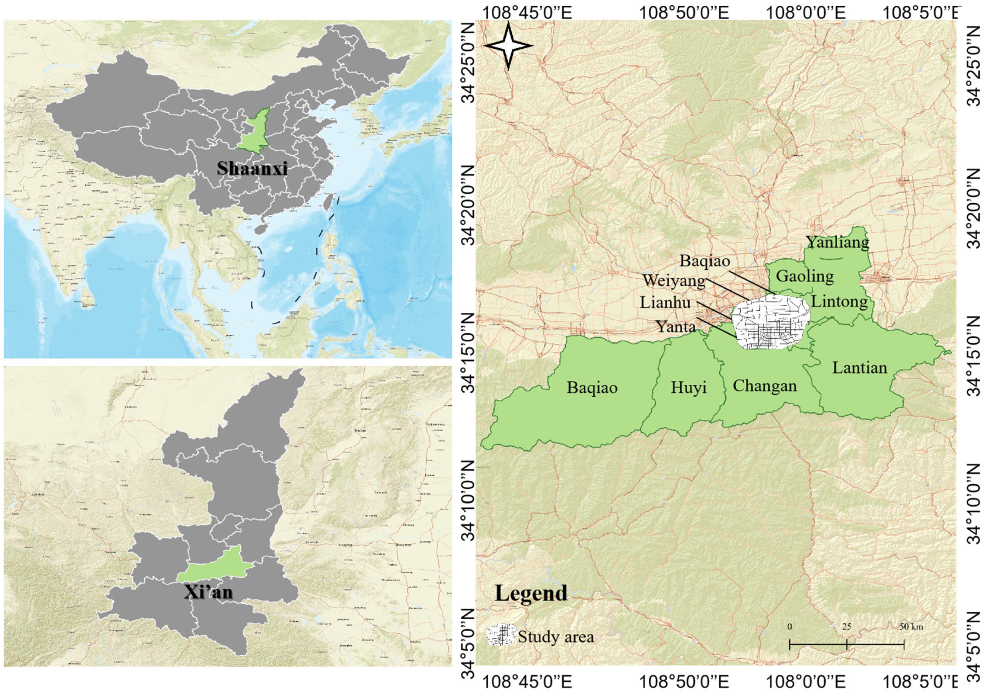
Figure 1. Study area.
Ijgi 14 00333 g001
Figure 2. Illustration of TAZs with road networks, POIs, and others spatial variables.
Ijgi 14 00333 g002
Figure 3. Spatial Distribution of Daily Turnover Rate per Active Bike in Xi’an.
Ijgi 14 00333 g003
Figure 4. Scatter Plot of Predicted vs. Actual Economic Performance Index for the XGBoost Model on the Test Set.
Ijgi 14 00333 g004
Figure 5. (a) Comparison of Model Performance Metrics. (b) Taylor Diagram Illustrating the Skill of the XGBoost and Baseline Models in Predicting the Economic Performance Index.
Ijgi 14 00333 g005
Figure 6. (a) SHAP Summary of Feature Impacts on Economic Performance Index. (b) SHAP Summary of Feature Impacts on Economic Performance Index.
Ijgi 14 00333 g006
Figure 7. (a). SHAP Dependence Plot: Non-linear Impact of Bike Supply Density on the Economic Performance Index (Interaction Feature: Proximity to Public Transit). (b) SHAP Dependence Plot: Non-linear Impact of Commercial POI Density on the Economic Performance Index (Interaction Feature: Bike Supply Density). (c) SHAP Dependence Plot: Non-linear Impact of Residential Density on the Economic Performance Index (Interaction Feature: Bike Supply Density). (d) SHAP Dependence Plot: Non-linear Impact of Proximity to Public Transit on the Economic Performance Index (Interaction Feature: Bike Supply Density). (e) SHAP Dependence Plot: Non-linear Impact of Road Network Density on the Economic Performance Index (Interaction Feature: Bike Supply Density). (f) SHAP Dependence Plot: Non-linear Impact of Average Income on the Economic Performance Index (Interaction Feature: Bike Supply Density).
Ijgi 14 00333 g007aIjgi 14 00333 g007b
Figure 8. SHAP Interaction Heatmap.
Ijgi 14 00333 g008
Figure 9. SHAP Waterfall Plot.
Ijgi 14 00333 g009
Table 1. Raw bike-sharing operational data.
Data TypeKey AttributeDescriptionUnit/Format
Trip Detail Records (TDRs)order_idAnonymized unique identifier for each tripAlphanumeric String
user_idAnonymized unique identifier for each userAlphanumeric String
bike_idUnique identifier for each bikeAlphanumeric String
start_timeTimestamp of trip commencementYYYY-MM-DD HH:MM:SS (UTC+8)
end_timeTimestamp of trip conclusionYYYY-MM-DD HH:MM:SS (UTC+8)
start_lngLongitude of the trip’s originDecimal Degrees (WGS84)
start_latLatitude of the trip’s originDecimal Degrees (WGS84)
end_lngLongitude of the trip’s destinationDecimal Degrees (WGS84)
end_latLatitude of the trip’s destinationDecimal Degrees (WGS84)
distance_meterDistance of trip as recorded by the systemMeters (Integer)
duration_secDuration of the tripSeconds (Integer)
fee_yuanCost of the tripChinese Yuan (Decimal)
Real-time Vehicle Status (RVS) Databike_idUnique identifier for each bikeAlphanumeric String
timestampTimestamp of the RVS data pointYYYY-MM-DD HH:MM:SS (UTC+8)
current_lngCurrent longitude of the bikeDecimal Degrees (WGS84)
current_latCurrent latitude of the bikeDecimal Degrees (WGS84)
statusCode representing bike’s operational stateInteger
(1: available, 2: in-use, etc.)
Table 2. Selected Urban Built Environment Variables and Characteristics.
CategoryVariablesDescriptionPotential Influence on Bike-Sharing EPMsData Source
POI DensityCommercial POI DensityNumber of commercial establishments per km2Positive: Increases trip attractions/destinations, supports diverse needs.OpenStreetMap (OSM), Baidu Maps API, Commercial vendors
Recreational POI DensityNumber of parks, fitness centers, entertainment venues, etc., per km2Positive: Generates leisure-based trips, enhances area attractiveness.OSM, Local Government GIS Departments
Office/Employment POI DensityNumber of office buildings and major employment sites per km2Positive: Drives commuter trips (first/last mile).OSM, Business Databases, Planning Departments
Land UseLand Use Mix (Entropy Index)Statistical measure of the diversity of land uses within a TAZ.Positive: Facilitates shorter, multi-purpose trips; reduces reliance on cars.Municipal Planning Dept. (Zoning Maps), Remote Sensing
Proportion of Residential AreaPercentage of TAZ area primarily classified or used for residential purposes.Mixed: High origin potential (esp. AM peak), destination (PM peak).Municipal Planning Dept. (Zoning Maps)
Proportion of Commercial AreaPercentage of TAZ area primarily classified or used for commercial activities.Positive: High destination potential, supports daytime/evening activity.Municipal Planning Dept. (Zoning Maps)
DemographicsPopulation DensityNumber of inhabitants per km2.Positive: Larger potential user base for bike-sharing services.National Census Bureau, Local Statistical Yearbooks
Median Household Income (Proxy)Estimated or aggregated median household income level within the TAZ.Mixed: Higher income may mean more transport options, or higher willingness to pay.Census Bureau
Transport Infra.Density of Metro StationsNumber of operational metro/subway stations per km2 or within a defined buffer.Positive: Enhances first/last-mile connectivity to mass transit.Public Transport Authority GIS Data, OSM
Bike Lane DensityLength of dedicated or protected bike lanes per km2 of TAZ area or road network length.Positive: Improves cycling safety, comfort, and attractiveness.Municipal Transportation Dept., OSM
Road Intersection DensityNumber of road intersections (3-way or more) per km2.Positive: Generally, indicates better network permeability and accessibility.OSM, Digital Road Network Databases
Table 3. Comparison of Selected Data Normalization Techniques.
TechniqueFormulaOutput RangeMean & Std DevSensitivity to OutliersCommon Use Cases &
Considerations
Min-Max Scaling ( X X m i n ) ( X m a x X m i n ) [0, 1]VariableHighAlgorithms requiring feature inputs within a bounded range (e.g., some neural networks); image processing.
Z-score Standardization ( X μ ) σ UnboundedMean = 0
StdDev = 1
ModerateWidely used for algorithms assuming normally distributed data or sensitive to feature scales (e.g., PCA, SVM, linear regression, gradient-based optimization in XGBoost).
Robust Scaler X m e d i a n Q R UnboundedVariableLowSuitable for datasets containing significant outliers, as it uses percentiles (median and interquartile range) and is thus more robust to extreme values.
Log Transformation l o g ( X + c ) VariableVariableReduces effect of outliersApplied to positively skewed data to stabilize variance, reduce heteroscedasticity, and approximate a normal distribution; useful when relationships are multiplicative.
Table 4. Descriptive Statistics of Key Variables.
VariablesCountMeanStdMin0.250.50.75MaxVIF
Bike Supply Density20224.19913.7496.24114.11821.30329.88788.4731.837
Commercial POI Density20225.59517.1713.24412.23721.88933.9596.0162.154
Residential Density20233.70913.01212.31724.28831.25941.10775.1561.676
Proximity to Public Transit202512.349274.68852.159290.384473.1760.371994.4131.322
Road Network Density2025.2922.6521.0293.2035.0857.4759.9841.984
Average Income20211,175.3435034.4543150.4217771.43410,059.56913,444.79333,172.1672.453
Table 5. Optimal Hyperparameters for the XGBoost Model.
HyperparameterValue
n_estimators (Number of trees)250
learning_rate (Learning rate)0.05
max_depth (Max tree depth)6
subsample (Subsample ratio)0.8
colsample_bytree (Feature ratio)0.7
gamma (Min split loss)0.1
reg_alpha (L1 regularization)0.01
reg_lambda (L2 regularization)0.1
Disclaimer/Publisher’s Note: The statements, opinions and data contained in all publications are solely those of the individual author(s) and contributor(s) and not of MDPI and/or the editor(s). MDPI and/or the editor(s) disclaim responsibility for any injury to people or property resulting from any ideas, methods, instructions or products referred to in the content.