Article

Relationship Between Aggregation Index and Change in the Values of Some Landscape Metrics as a Function of Cell Neighborhood Choice

1
Department of Civil, Environmental and Mechanical Engineering, University of Trento, Via Mesiano 77, 38123 Trento, Italy
2
Department of Theoretical and Applied Sciences, Università degli Studi dell’Insubria, 21100 Varese, Italy
3
C3A, Center Agriculture Food Environment, University of Trento, Via E. Mach 1, 38098 S. Michele all’Adige (TN), Italy
*
Author to whom correspondence should be addressed.
ISPRS Int. J. Geo-Inf. 2025, 14(8), 304; https://doi.org/10.3390/ijgi14080304
Submission received: 22 June 2025 / Revised: 29 July 2025 / Accepted: 2 August 2025 / Published: 5 August 2025

Abstract

Landscape metrics are one of the main tools for studying changes in the landscape and the ecological structure of the territory. However, the calculation of some metrics yields significantly different values depending on the configuration of the “Cell neighborhood” (CN) used. This makes the comparison of different analysis results often impossible. In fact, although the metrics are defined in the same way for all software, the choice of a CN with four cells, which includes only the elements on the same row or column, or eight cells, which also includes the cells on the diagonal, changes their value. QGIS’ LecoS plugin uses the value eight while GRASS’ r.li module uses the value four and these values are not modifiable by users. A previous study has shown how the value of the CN used for the calculation of landscape metrics is rarely explicit in scientific publications and its value cannot always be deduced from the indication of the software used. The difference in value for the same metric depends on the CN configuration and on the compactness of the patches, which can be expressed through the Aggregation Index (AI), of the investigated landscape. The scope of this paper is to explore the possibility of deriving an analytical relationship between the Aggregation Index and the variation in the values of some landscape metrics as the CN varies. The numerical experiments carried out in this research demonstrate that it is possible to estimate the differences in landscape metrics evaluated with a four and eight CN configuration using polynomials only for few metrics and only for some intervals of AI values. This analysis combines different Free and Open Source Software (FOSS) systems: GRASS GIS for the creation of test maps and R landscapemetrics package for the calculation of landscape metrics and the successive statistical analysis.

1. Introduction

Landscape metrics have had a great influence in the study of landscape change at different scales, from the local to the planetary. They have allowed for a different and more objective description, study and consideration of the landscape changes occurred through time in any given area of the world [1,2,3]. In the Anthropocene era we are living in, landscape change (e.g., due to deforestation or urbanization) is one of the major phenomenon that can be observed [4,5,6,7,8]. The concept of habitat loss and habitat fragmentation were certainly clear for the biologists, foresters and naturalists who worked in the field [9] but, due to a lack of clear quantification methods, they were less understandable for other scientists like engineers and mathematics because they were perceived as too qualitative. Landscape metrics combined with GIS techniques provide a tool to measure and quantify landscape, transforming this concept from qualitative to quantitative and helping to understand the concept of habitat fragmentation and to widen its adoption in ecology. This has created a new research field [10] and it is gaining popularity in education [11,12].
Landscape metrics are now a standard instrument for those who investigate landscape change dynamics in ecology [2,13,14,15,16,17,18,19] as well as in many other disciplines such as soil protection [20,21], water management [22,23,24,25], urban green spaces management [26,27,28,29] and disease spread [30]. For example in a recent review paper of the ecological restoration in Brazilian biomes, Guerra et al. [31] highlighted the need to expand research to assess landscape metrics to fill the gaps in research and helping prioritization, legislation and public policies. Some metrics like Patch Number (NP) or Mean Patch Size (MPS) are considered particularly robust and significant [32] and are extensively used in scientific literature [2,33] becoming a standard to compare different landscapes. New landscape metrics are currently proposed, such as the Ecological Land Evolution Index (ELEI) [34]. However, conceptual errors in the interpretation of landscape patterns, the intrinsic restrictions of landscape indices and inappropriate pattern index usage are well known limitations in the use of landscape metrics [35].
Although theoretically the calculation of these indices on the same data, given the same algorithm, should provide the same results, it has been proven that the lack of description of some parameters may affect the interpretation of the output in a dramatic way [32]. In fact, many scientific papers fail to describe in detail some important parameters, making it very difficult to correctly compare the results of different research even if they have been carried out in the same areas and/or using, at least apparently, exactly the same methods. In particular, the “Cell neighborhood” (CN) size is one of the most sensible parameters and Zatelli et al. [32] found that using a different software gives a different visibility to the setting of cell neighborhood size. Thus, when comparing different research works, it is extremely important to find a way to detect if the results are really comparable and in particular if landscape metrics have been evaluated using the same CN configuration.
Zatelli et al. [32] demonstrated that it is possible to use the values of the Aggregation Index (AI) to assess how the uncertainty on CN can affect some landscape metrics. This paper takes a step further, investigating the possibility of evaluating the influence of the choice of the CN value on the most frequently used landscape metrics. Moreover, a method to compute the differences between metrics evaluated with different CN is presented. These results can be used in two ways: (i) it is possible to estimate the difference in the metrics’ values with different CN configurations and, therefore, to assess the feasibility of using their values when the CN in use is unknown if the difference is small, and (ii) to evaluate the value of metrics with one CN configuration when the value for the other CN configuration is known but the map used to calculate them is not available.
The research question is, therefore, is it possible to estimate the differences in landscape metrics evaluated with a four and eight CN configuration using polynomials?
The paper is organized as follows: Section 2 introduces the Aggregation Index (AI) following the original formulation from He et al. [36], Section 3 describes the materials and methods used for the analysis, Section 4 illustrates the results that are discussed in Section 5 and finally the conclusions and future developments are presented in Section 6.

2. Aggregation Index

The Aggregation Index (AI) landscape metric has been introduced by He et al. in [36] as a way to quantify the presence of clusters in landscape patterns. Unlike its precursors contagion index (CI) and shape index (SI), AI is not affected by spatial patterning, landscape composition and patches’ shape. Moreover, AI is class specific, while CI evaluates the overall aggregation of the landscape combining all the classes. AI is defined as a ratio; therefore, it is independent from the scale or the map unit. This makes AI suitable not only for the comparison of the aggregation of different classes on the same map, but also for the examination of the same class on the same map at different resolutions.
The Aggregation Index (AI), formulated for raster data, is defined as the ratio between the total number of edges between pixels of the class and the maximum number of possible edges between pixels of the class [36]. Defining e i , j as the number of edges between cells of classes i and j, the number of total edges between cells of the same class is e i , i . It is possible to define a level of aggregation of class i as the ratio between the total number of edges between cells of classes i and the total area A i of this class, e i , i / A i . For a given value of A i , the maximum aggregation level, max e i , i / A i , corresponds to a configuration with a single clump of class A with the maximum value of e i , i , max e i , i .
For a four CN configuration, the value of max e i , i can be calculated with reference to the number n of pixels in the side of the largest square with area smaller than A i . If the class consists of a single square patch, n is the number of pixels on each side. In general, it is possible to define m = A i n 2 , the difference between the area A i of the patch and the area of the area of the largest square with area smaller than A i , and to evaluate the maximum number of edges between cells of the class A i , max e i , i , as
max e i , i = 2 n n 1 when m = 0 or max e i , i = 2 n n 1 + 2 m 1 when m n or max e i , i = 2 n n 1 + 2 m 2 when m > n
The original definition in He et al. [36] has m 0 as condition for the third line in Equation (1), but it is an obvious typo, and makes the case m = n mistakenly correspond to the third instead of the second line in Equation (1). Implementations in popular software for AI evaluation, such as FRAGSTATS and R’s landscapemetrics use the correct formulation in Equation (1) [37,38].
Finally, the Aggregation Index (AI) for class i is defined as
A I = e i , i max e i , i
AI ranges from 0, e i , i = 0 , i.e., there is no common edge between cells of class i and all cells of this class are isolated, to 1, when e i , i = max e i , i . In many implementations AI is expressed as a percentage by multiplying the ratio of Equation (2) by 100.
A I = e i , i max e i , i 100
The range for AI values is, therefore, between 0 and 100. All AI values in this paper use the definition in Equation (3) and are expressed as percentages.
Using an eight CN configuration leads to different values of number of total edges between cells of the same class e i , i and max e i , i , but their ratio, and therefore AI, remains the same.
AI is class specific, but an overall Landscape Aggregation Index ( A I L ) can be defined as the sum of all the AIs for each class A I i weighted by their percentage area A i % with respect to the total area of the map [36]:
A I L = i = 1 n A I i A i %
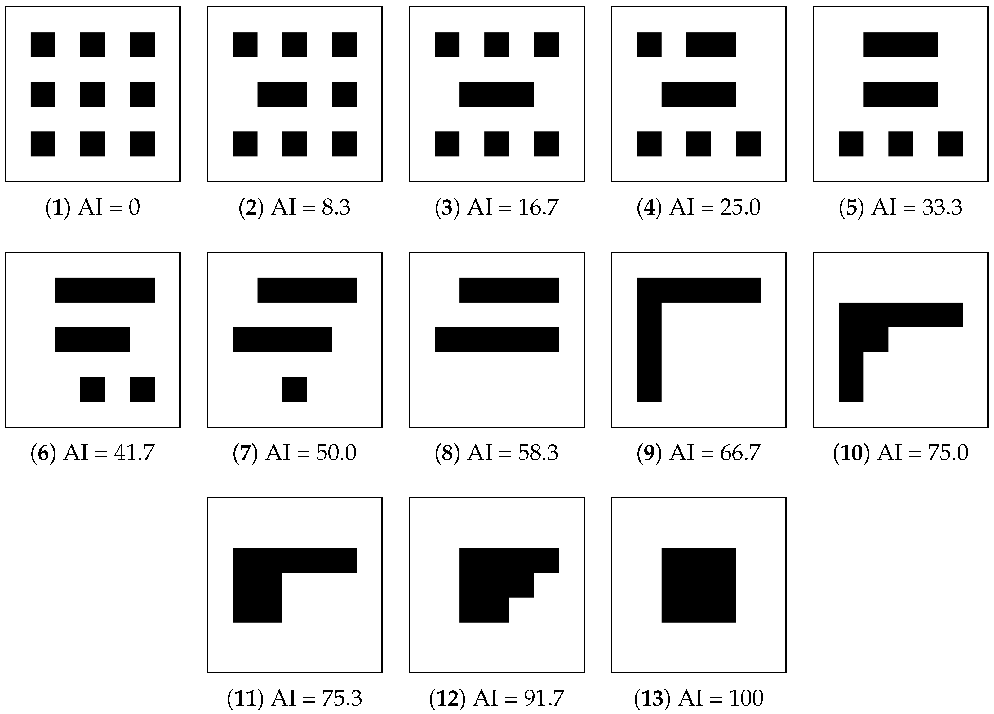
The behavior of AI for different map configurations has been tested with respect to aggregation, number of patches and spatial resolutions. Following He et al. [36], the evaluation of the response of AI to different levels of aggregation is performed using a binary map with a resolution 1 ([pixel]) containing 7 × 7 cells. The initial configuration contains nine isolated patches of 1 cell with a value of 1 and 40 background cells with a value of 0. The level of aggregation is then increased by incrementing the number of shared edges by one at a time, up to the final configuration where all the cells with a value of 1 are clumped in a single square (Figure 1).
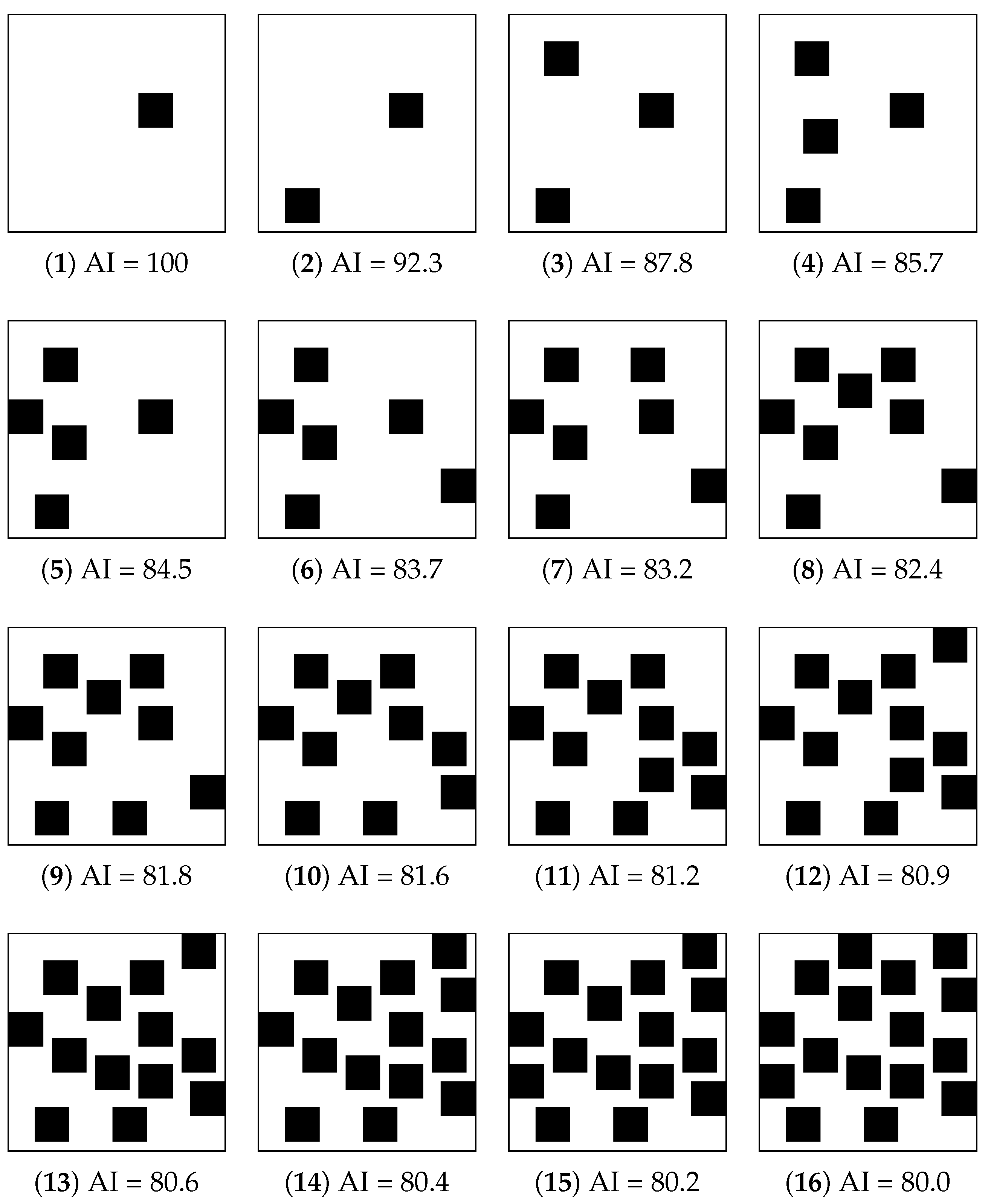
A second set of maps is created with patches of the same size added at random locations. The map is 25 × 25 cells with a resolution 1 ([pixel]) and the patches have size 4 × 4 cells. Patches are added one by one without overlapping nor touching, up to 16 total patches (Figure 2). Since patch size remains constant and the number of pixels of class 1 increases, AI decreases, but the decrement is not linear with the number of patches. Note that the positions of the patches are not relevant, as long as the patches remain separate, because the number of edges between cells, and therefore AI, remains the same.
Maps in Figure 2 differ from those in He et al. [36] because the random sequence that places the patches is different. Since only the number of patches and not their locations influences the value of AI, its values should be the same as in He et al. [36].
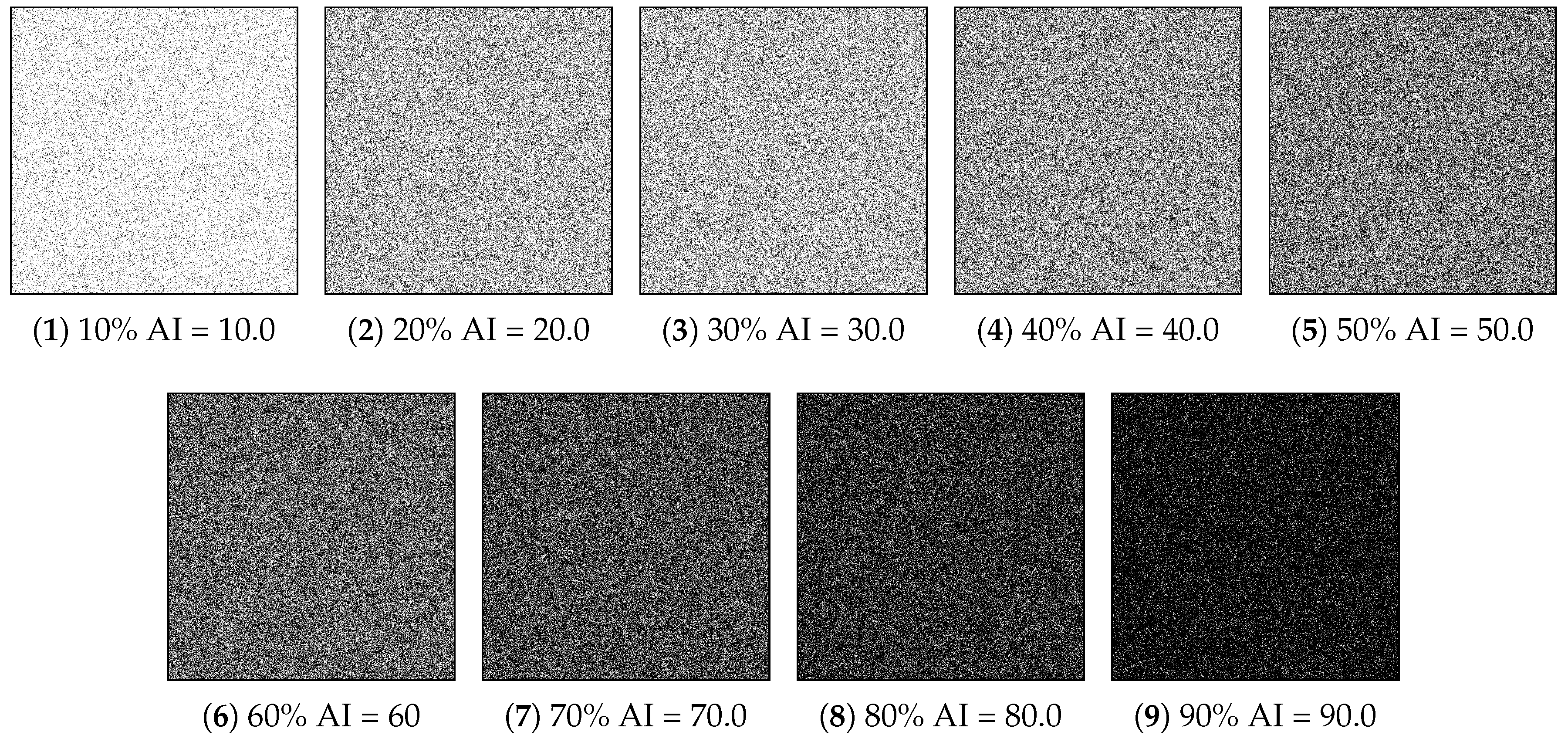
A third map set from He et al. [36] is composed of binary maps (Figure 3), 1024 × 1024 cells, which have an increasing number of randomly placed cells of value 1, from 10% to 90% of the whole area with 10% increments. For each map, AI values correspond to the percentage of cells with a value of 1.
The approximation functions that express the relationship between the AI and the variation in the values of some metrics with different CN configurations will be checked using these maps.

3. Materials and Methods

The analysis of the variation in AI in landscape metrics has been investigated using R’s landscapemetrics package [38] (Section 3.2), while test map creation has been scripted in GRASS GIS (Section 3.1). A series of maps have been created to examine the relationship between AI and the variation in landscape metrics.
The first set of maps consists of ten artificial maps with an increasing number of randomly placed cells, from 10% to 90% of the whole area, with 10% increments (Figure 3). These maps have been used to estimate the coefficients of approximating functions expressing the relationship between the AI and the difference in the values of some metrics with different CN configurations.
A second set of artificial maps has been created to check the approximating functions. These maps (Figure 2), in part, correspond to the maps used in He et al. [36] to test AI response to the maps’ features such as level of aggregation, number of patches and spatial resolutions.
The third set of maps, represented in Section 3.3, is based on a real forest map, with the application of a high-pass filter and low-pass filter to create a series of maps with increasing levels of aggregation. These maps will be used to test the viability of using the approximating functions for real maps.

3.1. Test Software

The evaluation of all the landscape metrics, including AI, has been carried out using R’s landscapemetrics package [38]. R is a Free and Open Source Software (FOSS) environment for statistical computing and graphics [39]. The landscapemetrics package evaluates landscape metrics for raster maps (“objects” in R). It implements most of the original metrics from FRAGSTATS [37] plus some new metrics following recent developments in the field. It can also be used to build new custom metrics. It is possible to use this package to visualize the results of the analysis [38].
GRASS GIS [40] is a multi-purpose FOSS GIS for geospatial data production, analysis and mapping [41] available under the GNU Public License (GPL), and is used in research and education [11]. Ready-to-install packages are provided for the MS Windows, Apple Mac OSX and Linux operative systems. It is a project of the Open Source Geospatial Foundation (OSGeo). It has been used to script the creation of the artificial maps and maps derived from real maps.
The Landscapemetrics package performs all the operations about landscape metrics that are possible on Fragstat [38], with the option of using a 4 or 8 CN. It can be used to calculate an entire set of metrics (cell, class or whole landscape). It also accepts as input a user defined array of metrics to be calculated.
Landscapemetrics is based on Fragstat, so all the metrics that are used in the literature are available from this package [38]. The choice of other tools for landscape metrics evaluation would have been limiting, for example, in QGIS [42] the Lecos plugin [43] calculates only a limited array of metrics, while the r.le suite in GRASS GIS does not allow an 8 CN [32].

3.2. Landscape Metrics Calculation with R

A custom R script has been written to calculate the metrics for a set of maps, using both 4 CN and 8 CN configurations. The results of these calculations are stored in two different dataframes, which contain a row for each metric and a column for each map, with one containing the metrics values with a 4 CN and one containing the metrics values with an 8 CN. The second step performed by the R script is to subtract these two dataframes to quantify the differences in absolute value and in percentage for the two CN configurations. The differences can then be easily plotted and analyzed. The coefficients and the fitting statistics for 3-degree and 6-degree polynomials as a function of AI are evaluated for each metric difference. Finally, the differences for the area_mn metric for binary maps in Figure 3 between interpolated and evaluated values with an 8 CN are calculated to check the interpolated values.
The whole procedure is shown in the flowchart in Figure 4.
The script is available on a dedicated GitHub repository under the GNU license [44].

3.3. Maps

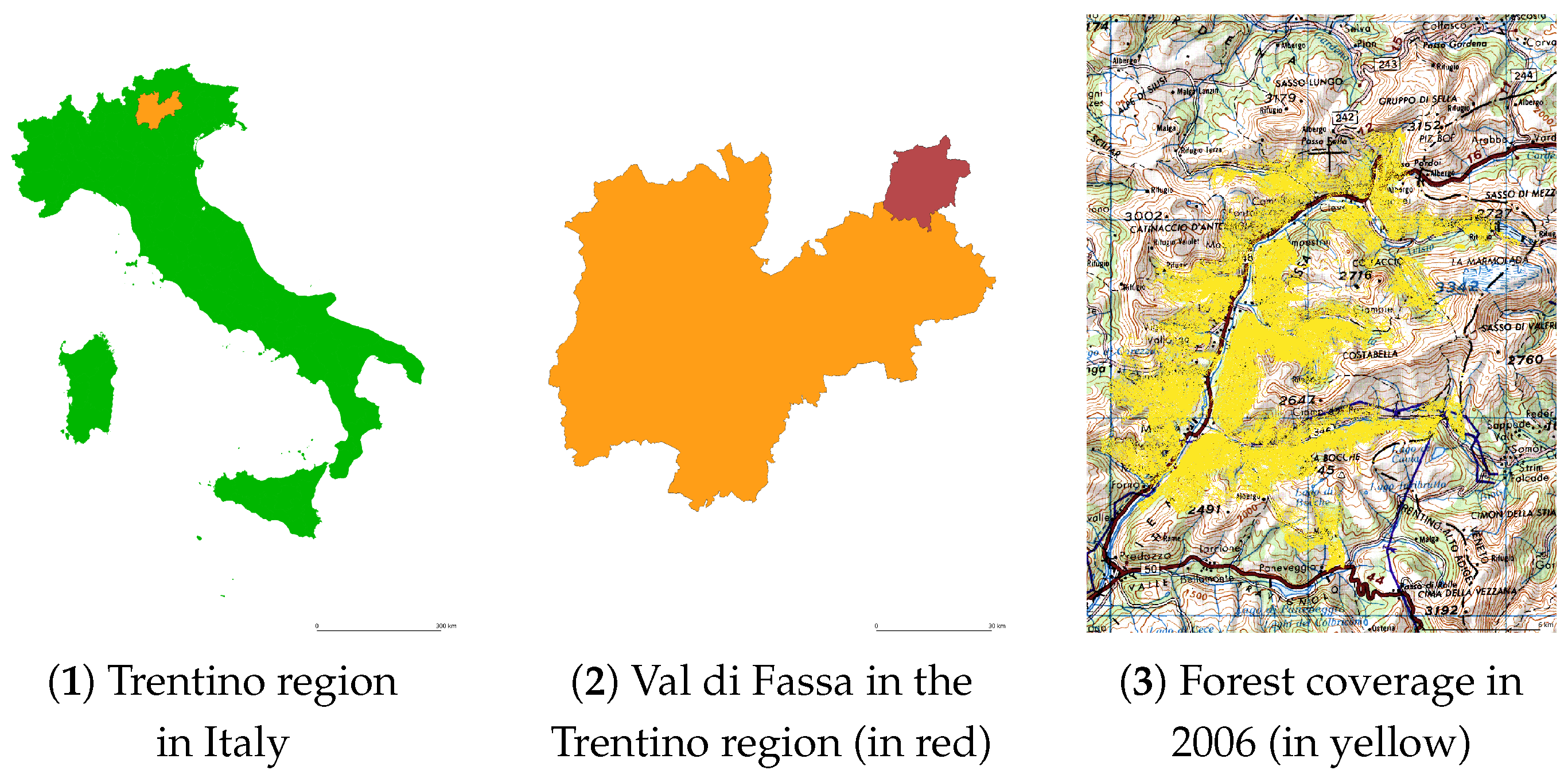
A set of maps have been built by applying filters to a real map of the forest coverage in the Val di Fassa, Italy, in 2006 (Figure 5(3)). This map has already been used to test the relevance of the cell neighborhood size in landscape metric evaluation in [32]. Val di Fassa is a valley in the north east of the Trentino region in the Alps in Northern Italy (Figure 5). A considerable expansion of the forested area has been registered in this area in the last century [2,38,45,46,47]. This trend is currently being analyzed in the Trentinoland project, investigating the forest coverage evolution of the whole Trentino region in Northern Italy [48].
The area covered by this map is 567.28 km 2 (56,728 ha), of which 132.36 km 2 (13,236 ha, 23.33%) were covered by forest in 2006. The region boundaries are 5157094 N, 5132029 S, 721983 E, 699351 W, in the ETRS89/UTM 32 N (EPSG 25832) datum. The raster map has a 10 m resolution, with 2509 rows and 2265 columns, for a total of 5,682,885 cells. The map is binary, with a value of 1 representing forest and a NULL value for other coverages.
To obtain maps with AI values covering the 0–100 range as much as possible, two sets of maps have been created from the original forest map. All the new maps cover the same area and have the same resolution of the original one.
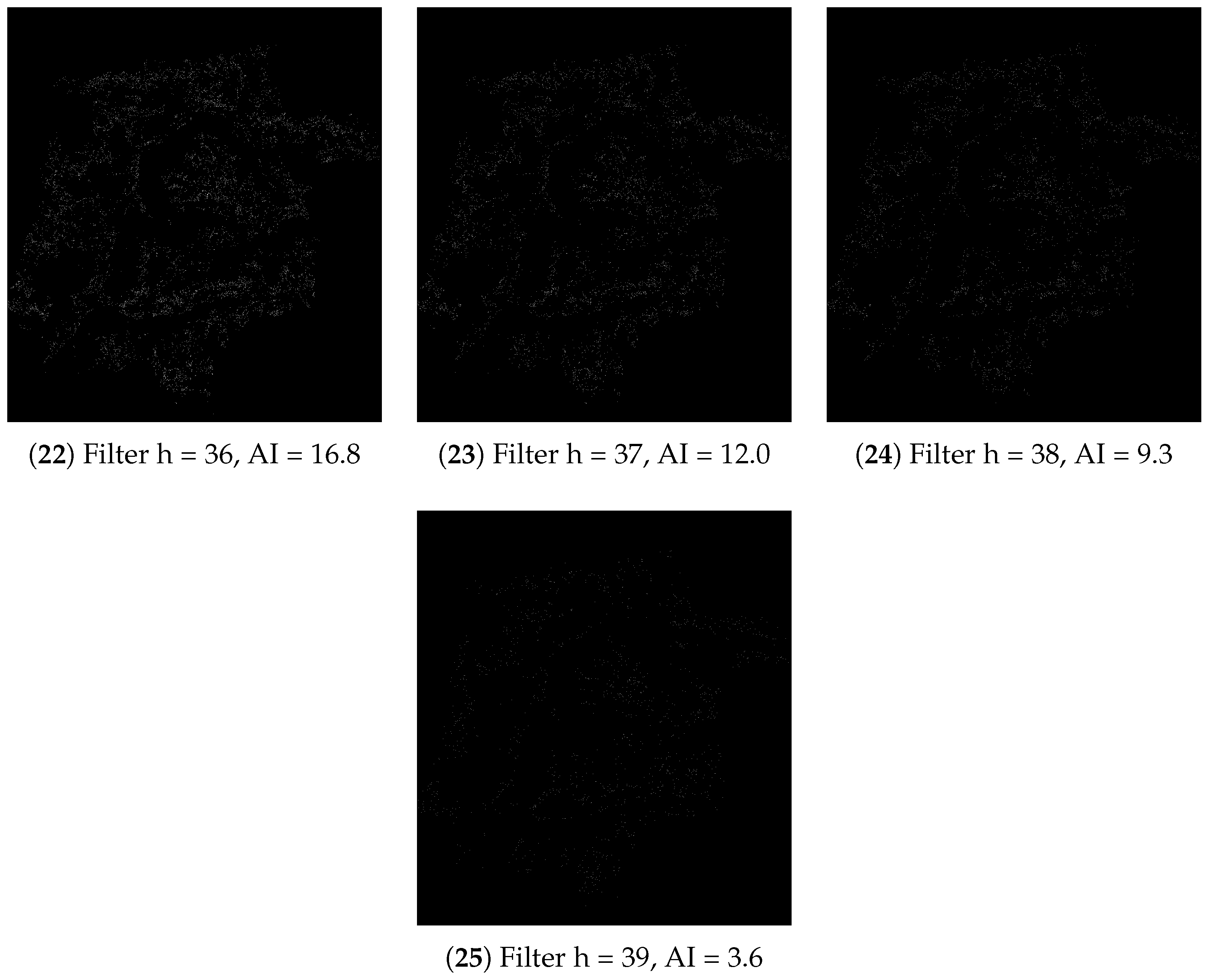
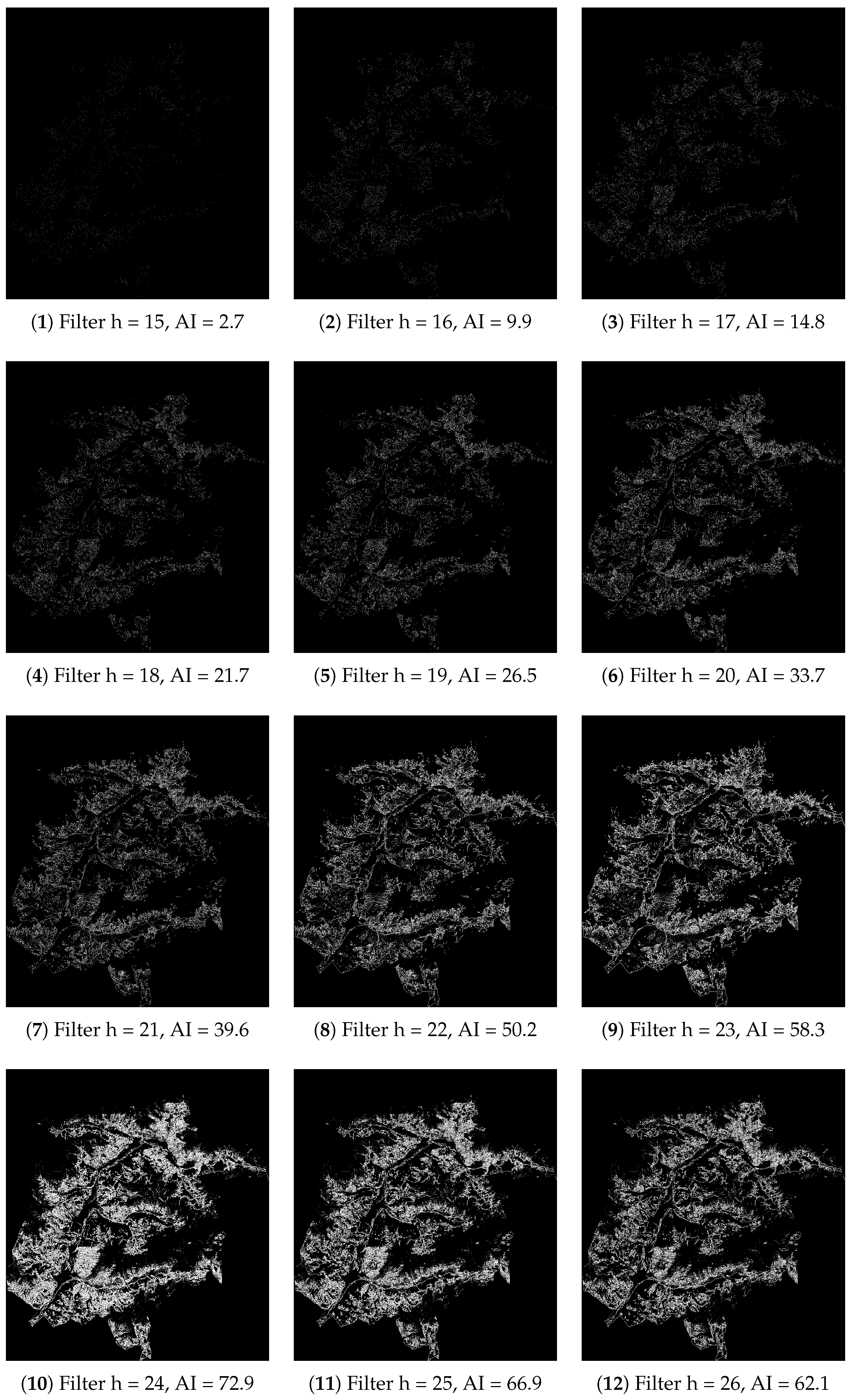
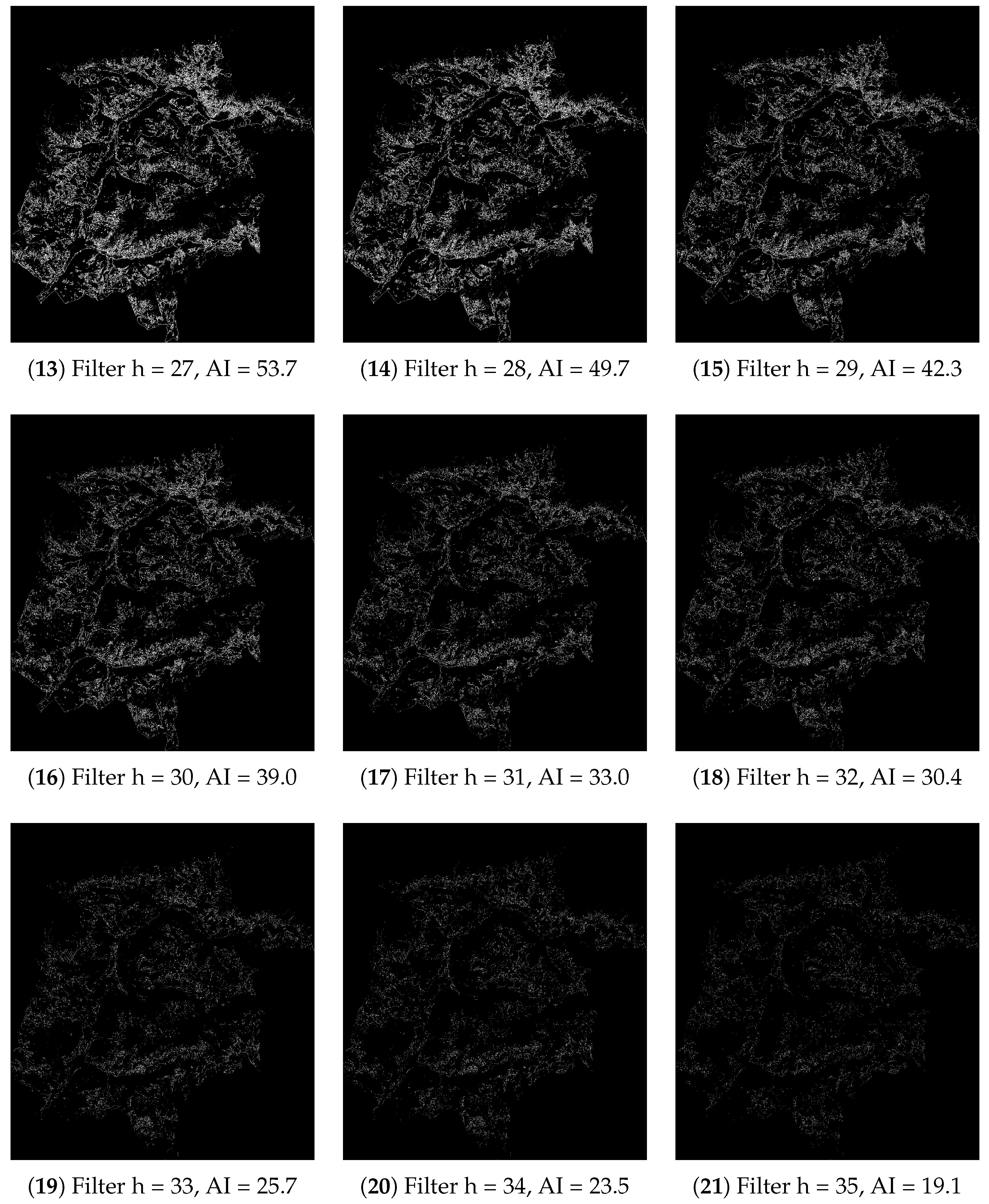
The first set of maps has been created by applying a 5 × 5 high-pass filter, with central value from 15 to 40 and with step 1 (Table 1). All pixels with a value of 5 or above are set to 1, and the remaining pixels are set to 0. The resulting set contains 25 maps with AI values between 2.7 and 72.9. Images are shown in Figure A1 in Appendix A.
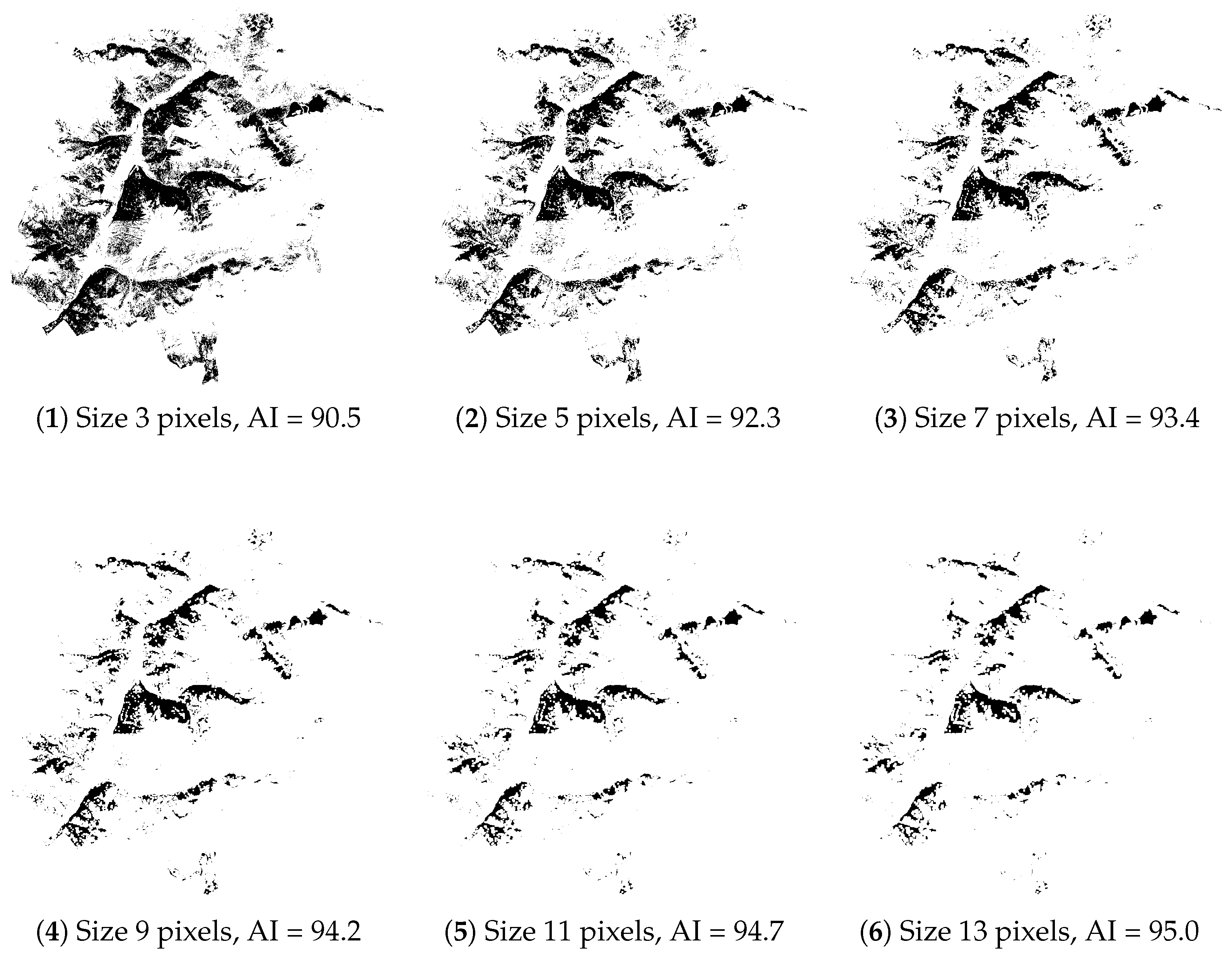
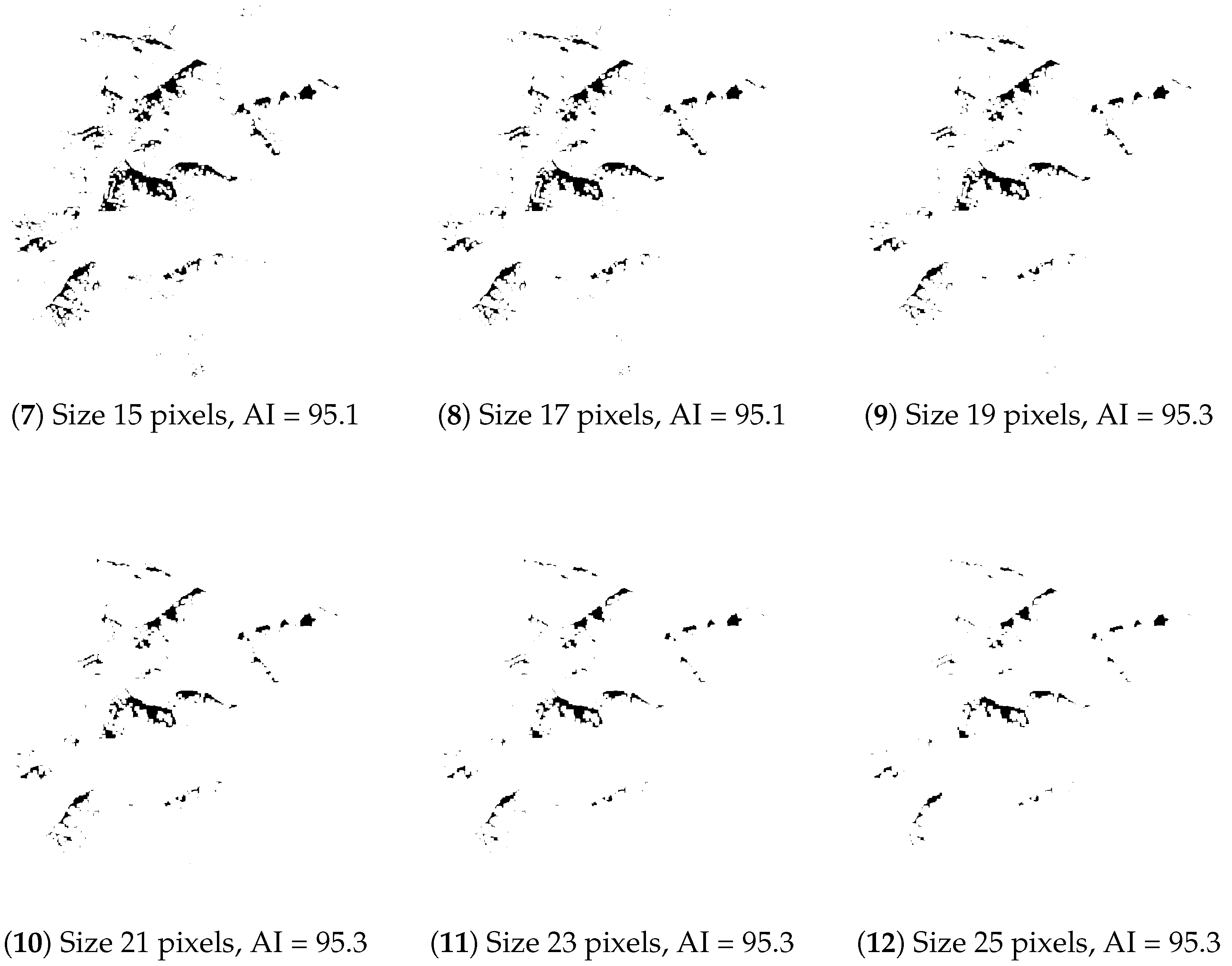
The second set contains thirteen maps, created by a moving window assigning the mode of the values to the central pixels. The size of the moving window varies from 3 to 25, using only odd numbers. For these maps AI ranges from 90.5 to 95.3. Images are shown in Figure A2 in Appendix A.
The union of these two map sets contains maps with AI values ranging from 2.7 to 95.3, providing a good sampling for the whole 0–100 variation interval for AI.

4. Results

Landscape metrics discussed in Section 3.2 have been evaluated for the test maps described in Section 2 and Section 3.3. All the maps are binary and all the landscape metrics have been evaluated for the class of a value of 1. This approach allows the isolation of the effects of different CN configurations on the metrics values from the influence of the presence of different classes with different metrics values.
All the metrics have been calculated using both four and eight CN configurations to assess the influence of this choice on the metrics values as a function of AI.

4.1. Metrics Selection

Landscape metrics whose values depend on the choice of CN have been selected by comparing their values when evaluated with a four or an eight CN configuration using R’s landscapemetrics package [32]. Metrics which are evaluated as ratios are independent from the choice of CN [32], because numerators and denominators change in the same way when the choice of CN changes.
The result is shown in Table 2. The same table indicates the abbreviate names of the metrics used by R’s Landscapemetrics. These abbreviations will be used in the next sections.
The landscape metrics cohesion, frac_mn, pafrac, para_mn and shape_mn have not been used in the proceeding of this research because their evaluation is too memory intensive and would have required huge processing times.
Note that different software implementations use slightly different metric names.

4.2. Artificial Maps

Because the maps in He et al. [36] appear to be out of sequence and AI values seem dubious, AI values for maps in Section 2 have been re-evaluated using AI definition of Equation (3) and a four CN configuration.
Values of AI for the first set of maps (Figure 1) correspond to the values reported in He et al. [36].
The second set of maps has been created by adding randomly placed non overlapping 4 × 4 patches on a map of 25 × 25 cells with resolution 1 ([pixel]), from 1 to 16 patches (Figure 2). AI decreases when the number of patches increases, as shown in Table 3. In this table e 1 , 1 is the number of edges between cells with a value of 1 (in black on Figure 2), n is the number of pixels in the side of the largest square with area smaller than A i and m = A i n 2 , as defined in Section 2. max e 1 , 1 is evaluated with Equation (1) and AI with Equation (3). The last column “Corresponds” indicates the correspondence with values reported in He et al. [36]. The AI value for the map in Figure 2(6) does not correspond, the value has probably been erroneously copied for the preceding one; * denotes values that are swapped in the original figure in He et al. [36].
AI values for the third map set from He et al. [36] (Figure 3), correspond to the percentage of cells with a value of 1, from 10% to 90% of the whole area with 10% increments. For these maps all the landscape metrics whose values depends on the CN choice have been evaluated and their values will be used to test polynomial functions to evaluate the differences in metrics values for different CN configurations. Landscape metric values are reported in Table A1 and Table A2 for CN configurations equal to four and in Table A3 and Table A4 for CN configurations equal to eight in Appendix B.1.

4.3. Real Maps

The fourth set of maps represent a modification of real forest maps, described in Section 3.3, with AI ranging from 2.70 to 95.3. The original forest map has an AI value of 86.7. Maps created using the low-pass filter described in Section 3.3 have AI values from 2.7 to 72.8, while maps resulting from the application of a low-pass filter range from 86.7 to 95.3 (Table 4).
Metrics which have different values for four CN and eight CN configurations (see Section 4.1) have been evaluated for all the maps (Table A1, Table A2, Table A3, Table A4, Table A5, Table A6, Table A7 and Table A8 in the Appendix B.1 and Appendix B.2). Then the difference for each map and each metric is evaluated as the value of the metric calculated with an eight CN configuration minus the value of the same metric using a four CN configuration (Table A9, Table A10, Table A11 and Table A12 in Appendix B.3).
The first result is that for 8 of the metrics out of 13, the differences are mostly positive (area_mn, cai_mn, contig_mn, dcore_mn, enm_mn, gyrate_mn, lpi and mesh), i.e., the value of the metric is mostly higher when calculated with an eight CN configuration, while for the other 4 metrics (division, np, pd, split), the differences are negative. This provides a hint on the expected behavior of the differences between metrics when AI varies. With increasing AI values the landscape becomes more aggregated; therefore, the difference between the two CN configurations should decrease. However, not all the metrics follow this trend. Furthermore, for most of the maps, regular behavior is not recognizable, nor can a general rule to forecast how the difference will behave be inferred. Most of the metrics are very unstable with respect to AI values.
This emphasizes once more how crucial it is to understand which CN configuration has been used when comparing findings from different research that employ landscape metrics.

4.4. Polynomial Approximation

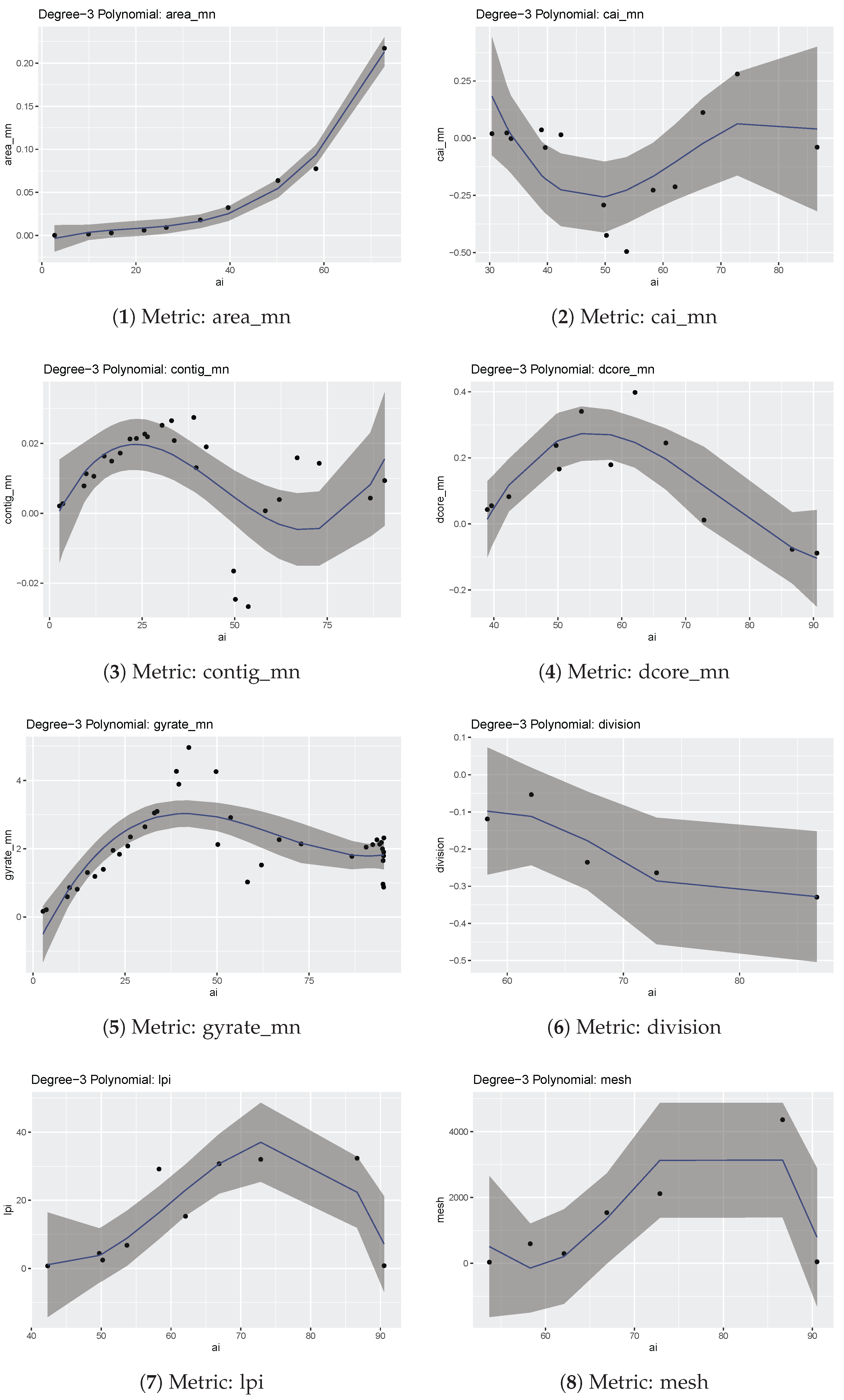
The coefficients and relevant statistics have been evaluated for 3 and 6-degree polynomials for the differences in each metric. The choice of the polynomial degrees depends on the following considerations: (i) a polynomial of 3 degrees is simple and fast to use, (ii) polynomials of 4 and 5 degrees do not provide tangible benefits with respect to 3-degree polynomial and (iii) the use of polynomials with an order above six is impossible for most of the metrics differences because the number of data points is limited. Since metric differences are non zero only on some intervals, which change for each metric, only the values where the differences are non-null have been used for the interpolation. Figure 6 illustrates this for metric cai_mn: when the whole 0–100 range is used for AI and also for values where the differences are null, with AI below 30, and where the difference behavior is very unstable, with AI above 90, they are used to estimate the interpolation coefficients. Therefore, to avoid the influence of the values in these intervals, only differences in the AI interval 30–90 are used. The interval boundaries for each metric are reported in Table 5 and Table 6.
Both 3 and 6 degrees coefficients polynomials have been tested to assess whether low-degree polynomials can provide a sufficient approximation with a smaller number of coefficients. Results are reported in Table 5 and Table 6, while information to assess the goodness of fit is in Table 7 and Table 8.
The interval for the metric division contains only five values (maps), thus the coefficients for a 6-degree polynomial cannot be evaluated: for this reason its coefficients and statistics are not reported in Table 6 and Table 8.
The interval chosen for the polynomial interpolation of the metric mesh contains only seven values, the same number of the unknowns for grade 6; therefore, no statistics is available.

5. Discussion

Results indicate that for values of AI above 90, the metric differences are either negligible or have an unpredictable behavior. Therefore, for very compact patches a small increment or decrement in the AI can lead to very different metric values regardless of the CN (four or eight) configuration choice. In this situation landscape metrics evaluated using the two configurations are simply impossible to compare.
In a similar way, for low AI values, metrics differences are usually null. However, the threshold below which this happens is different for every metric.
All the polynomial interpolations correspond to p-values for the F-test well below the chosen significance level of 5% (i.e., 0.05) (Table 7 and Table 8). Therefore both 3 and 6 degree polynomials provide a better fit to the metric differences than an intercept-only model. However, values of Multiple R-squared and Adjusted R-squared indicate that most of the 3-degree polynomials are not a good fit, while, as expected, using a 6-degree polynomial allows a better fit. Low Multiple R-squared values mean that most of the 3-degree polynomials do not provide a good model to predict the metrics differences. The same situation is indicated by low values of Adjusted R-squared, which incorporates the model’s degrees of freedom. The use of 6-degree polynomials provides more degrees of freedom, and therefore enhances the metric differences prediction, as indicated by higher values of Multiple R-squared and Adjusted R-squared.
Choosing a threshold value of 0.9 for the Adjusted R-squared values, only the area_mn and pd metric differences can be properly fitted by a 3-degree polynomial. With the same threshold and a 6-degree polynomial, five metrics differences can be fitted (area_mn, ndca, pd, np, enn_mn).
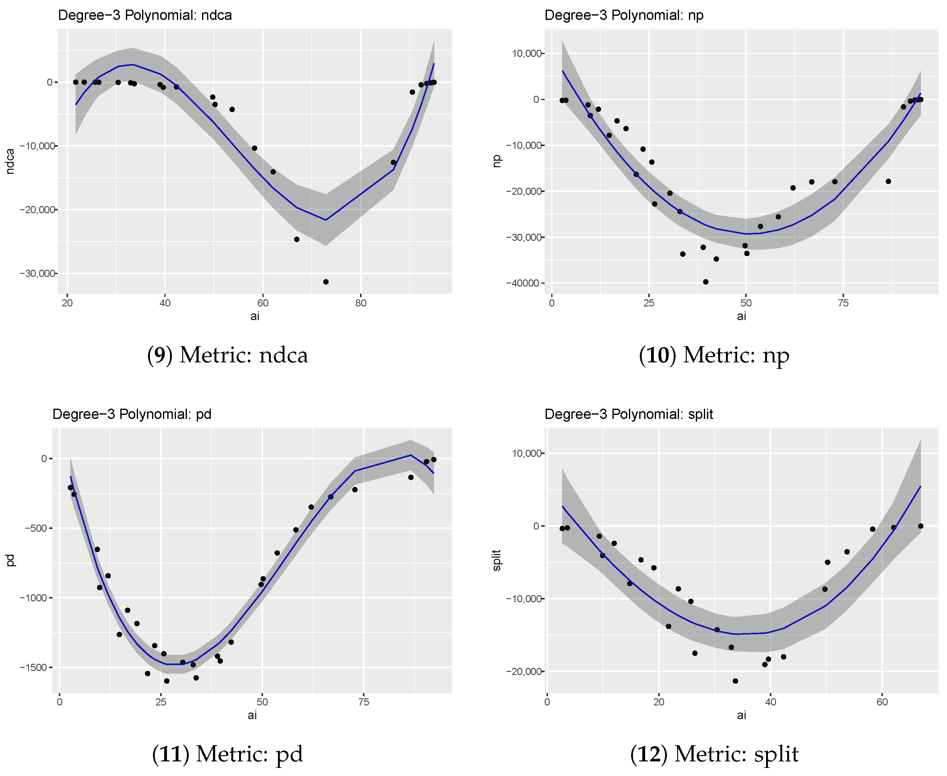
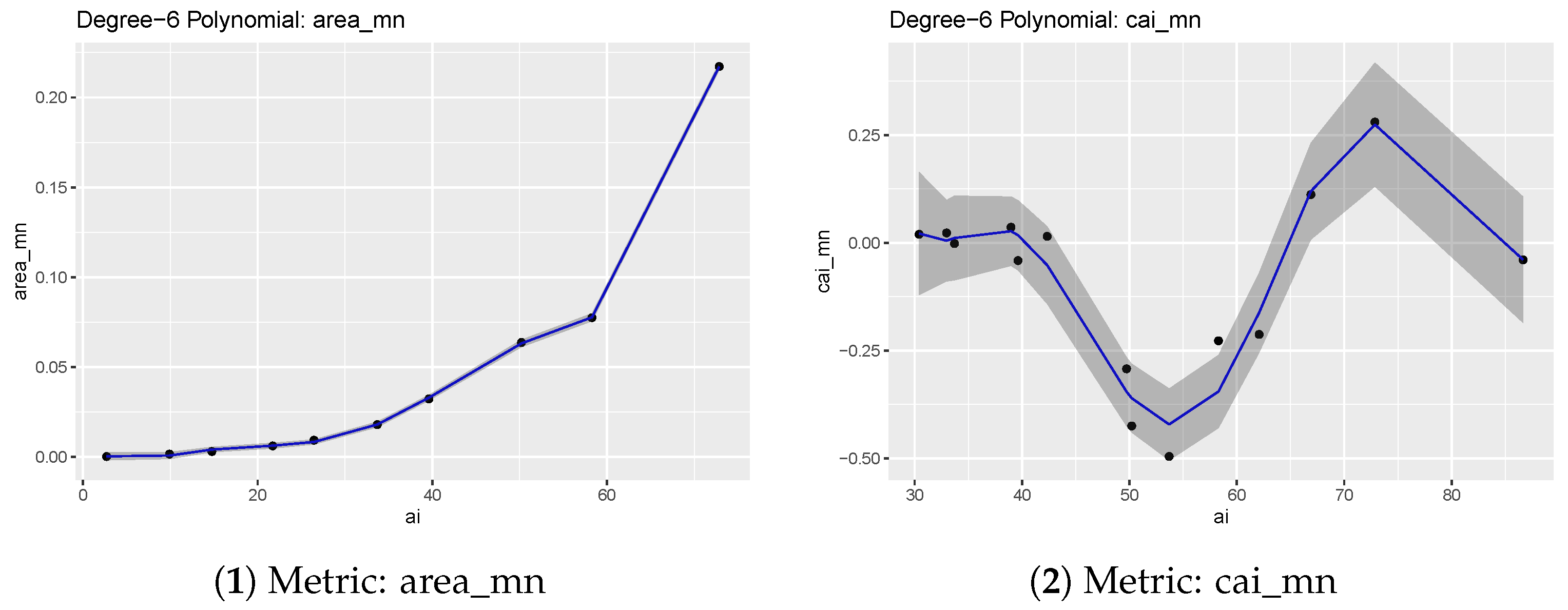
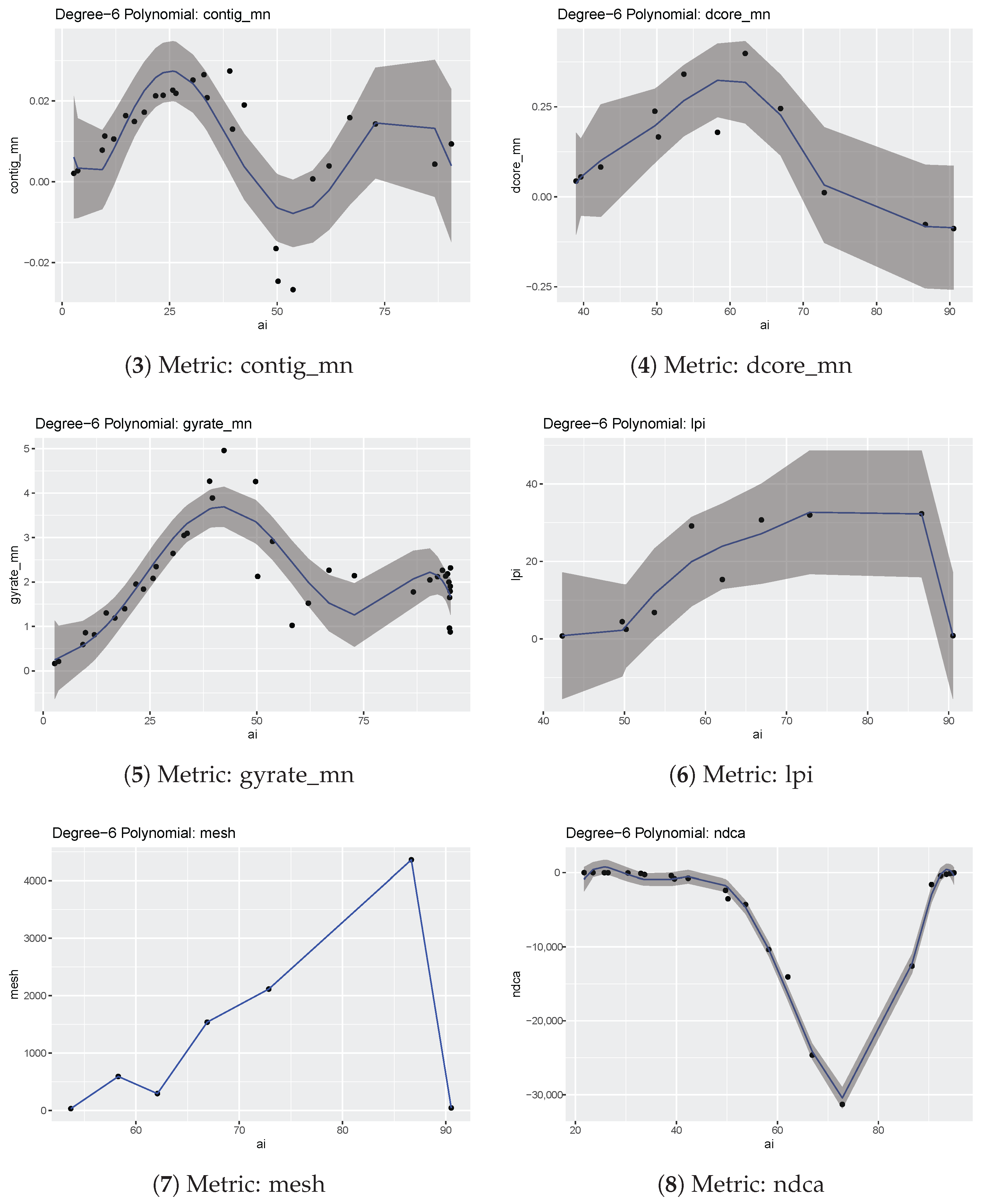
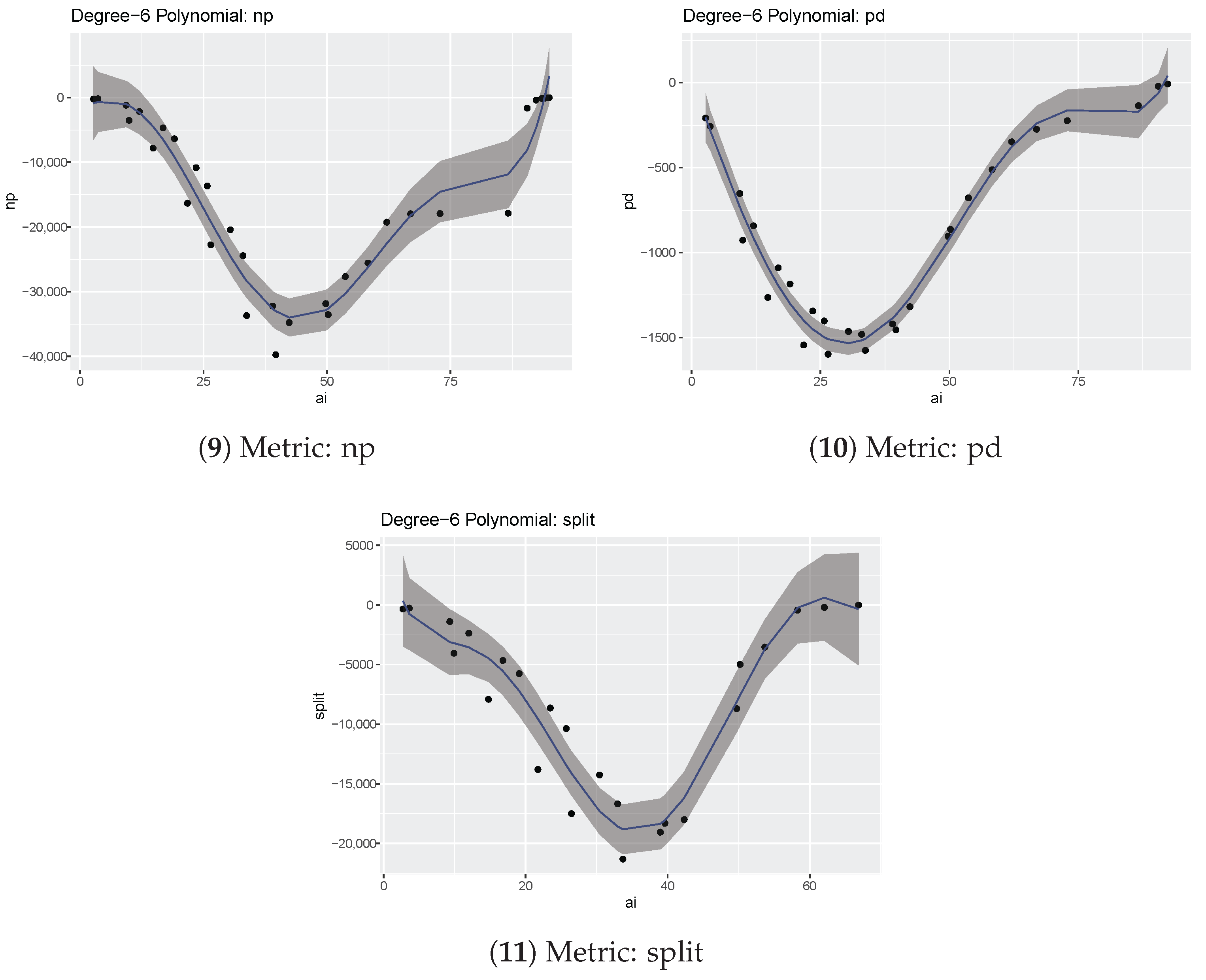
A visual representation of this is given by Figure A3 in Appendix C for 3-degree polynomials and in Figure A4 in Appendix D for 6-degree polynomials.
Differences behave differently for each landscape metric:
area_mn
Shows a parabolic trend up to AI equal to 86.65, then it becomes unstable; in the AI interval 0–86.65 it can be fitted by a 3-degree polynomial, with an Adjusted R-squared of 0.9835;
cai_mn
Differences are negligible up to AI = 30 and are unstable above 90, with a parabolic trend in between; overall they have a larger variability than other metrics differences; fit for 3-degree polynomial is poor, with an Adjusted R-squared of 0.2714, while the 6-degree polynomial fares better with an Adjusted R-squared of 0.8828;
contig_mn
Shows a sinusoidal behavior for AI below 90, with unpredictable behavior above this value; fitting by both 3-degrees (Adjusted R-squared 0.2523) and 6-degrees (Adjusted R-squared 0.5232) is poor; fitting by a sinusoidal function could be tested;
dcore_mn
Differences are negligible for AI below 34, then their trend becomes sinusoidal up to AI equal to 90, then it is unstable; Adjusted R-squared values are similar for the 3-degrees (0.6926) and 6-degrees (0.6921) polynomial, indicating a rather poor fitting;
division
Differences are null up to AI = 55, then their trend is parabolic, becoming unstable above 90; fitting with a 3-degree polynomial is very poor (Adjusted R-squared 0.3831), while it is not possible to use a 6-degree polynomial, as only five data points are available in the chosen interval;
enn_mn
In the interval 0–90, the 3-degree polynomial provides a poor fit (Adjusted R-squared 0.4727), but the 6-degree polynomial is good (Adjusted R-squared 0.9191);
gyrate_mn
Unstable above AI = 33, both 3-degrees (Adjusted R-squared 0.6926) and 6-degrees (Adjusted R-squared 0.8890) polynomials provide an almost good fit;
lpi
Differences are basically null outside the 45–90 AI interval, while inside this interval they have an oscillatory behavior; polynomial approximation is poor, with Adjusted R-squared 0.6653 for grade 3 and Adjusted R-squared 0.6606 for grade 6;
mesh
Differences have a parabolic trend in the 55–100 AI interval, and they are null outside; a 3-degree polynomial fit is poor (Adjusted R-squared 0.4727), while there are not enough data points to estimate the coefficients of the 6-degree polynomial;
ndca
Differences are negligible outside the 22–94 AI range; the 3-degree polynomial is not a good fit (Adjusted R-squared 0.7909) but the 6-degree polynomial is (Adjusted R-squared 0.9873);
np
Differences have a parabolic trend with oscillations and they are basically null for AI values above 94; the 3-degree polynomial is quite a good fit (Adjusted R-squared 0.8209), while the 6-degree polynomial provides a good fit (Adjusted R-squared 0.9192);
pd
Differences have a trend similar to those for the metric np, parabolic trend with oscillations and up to AI = 92; both 3-degree (Adjusted R-squared 0.9561) and 6-degree (Adjusted R-squared 0.9707) polynomials provide a good fit;
split
Differences are negligible for AI above 70, then the 3-degree polynomial is not a good fit (Adjusted R-squared 0.6991), while the 6-degree polynomial fares better (Adjusted R-squared 0.8890).
An overall view of the goodness of fit for landscape metrics approximations with 3- and 6-degree polynomials is provided in Table 9.
Table 9 shows that it is possible to fit the differences in three metrics, area_mn, enn_mn and pd, with both 3- and 6-degree polynomials. The differences in three more metrics, ndca, np and split, can be modeled using only 6-degree polynomials.
However, even for metrics with a good fit, metric difference evaluation using a polynomial does not provide reliable values. For example, Table 10 shows the differences for the area_mn metric for binary maps in Figure 3, with differences between interpolated and evaluated values with CN eight of more than 1000% for low AI values.

6. Conclusions

The paper tries to assess whether it is possible to infer the value of landscape metrics evaluated with a CN value when the value of the same metric is known in the other CN configuration. The results in Section 4 demonstrate that this is possible only for some metrics and only for selected value intervals. Many landscape metrics are inherently very unstable with respect to variation in the AI and this makes it difficult to model their behavior with polynomials. Therefore, the answer to the initial research question is that it is possible to estimate the differences in landscape metrics evaluated with a four and eight CN configuration using polynomials only for few metrics and only for some intervals of AI values. Even in these favorable cases, however, the estimation of the differences between CN configuration is very approximate.
The results highlight the importance of the choice of the CN in the evaluation of the landscape metrics, whose values can change in various orders of magnitude for different CN choices. Moreover, one important conclusion is that landscape metric values can be very unstable with respect to the patch configurations they try to describe; therefore, their use should always be integrated by other information under expert judgment.
The difficulty of comparing results from different studies using landscape metric remains, unless the used CN is known. Results in Section 5 can help, at least in indicating for each metric the intervals of AI values for which differences between CN are negligible. However, the need to always indicate the CN in use or at least the software used to evaluate the landscape metrics, from which the CN can be usually deducted, must be strongly emphasized.
The possibility of comparing landscape metrics between different studies is becoming more important because long time-series of Land Use/Land Coverage maps are becoming available [49], as the digitalization of a large number of historic maps is underway [50,51,52,53], with the development of automatic or semi-automatic digitalization procedures [54,55,56,57].
The limitations of this study concern the difficulty of creating maps with a dense and regular distribution of AI values, which would provide a larger sample size. This could also allow a better selection of the intervals where the creation of interpolating functions for the metrics differences is relevant. Moreover, only 3- and 6-degree polynomial fitting has been tested: different interpolating functions could be chosen, even using a different function for each metric. Another limitation lies in the impossibility to test the interpolating functions in real applications from third parties, as no example of landscape metrics evaluated with both four and eight CN configurations could be found in the literature.
During the numeric experiments carried out for this research it has emerged that the use of an eight CN configuration leads to a significant increase in computing resource demand, in particular in terms of memory (RAM), which can be a limiting factor for some applications.
Future developments include the creation of a set of maps with a higher resolution variation in AI in the parts of the 1–100 interval where metric differences are not null nor unstable, so that the use of approximating functions can be better investigated. Fractal landscapes could provide an effective way to generate these maps. The use of other functions than polynomials could be tested; for example, the contig_mn and dcore_mn metrics show a sinusoidal behavior for some AI intervals. Finally, the application of the polynomials to real cases where metrics have been evaluated with both CN configurations could be interesting, but so far the literature review has not provided any data of this type.
Author Contributions

Research conceptualization, Paolo Zatelli, Clara Tattoni and Marco Ciolli; methodology and software, Paolo Zatelli; validation, Paolo Zatelli and Marco Ciolli; writing–original draft preparation, Paolo Zatelli; writing–review and editing, Paolo Zatelli, Marco Ciolli and Clara Tattoni. All authors have read and agreed to the published version of the manuscript.

Funding

This research received no external funding.

Data Availability Statement

Test maps are available under the Creative Commons Attribution 4.0 International (CC-BY) license on Zenodo. The dataset contains the complete sets of synthetic maps used in Section 2 (Figure 1, Figure 2 and Figure 3) and the base map used in Section 3.3 to create the other maps with the filter described in the same section. Zatelli, P. (2025). Test images for the evaluation of the Aggregation Index [Data set]. Zenodo. https://doi.org/10.5281/zenodo.15422716.

Acknowledgments

The authors thank Stefano Gobbi for the initial discussion about landscape metrics differences evaluation and its draft R implementation.

Conflicts of Interest

The authors declare no conflicts of interest.

Abbreviations

    The following abbreviations are used in this manuscript:
AIAggregation Index
CNCell Neighborhood
EDEdge Density
GISGeographic Information System
GPLGnu Public License
FOSSFree and Open Source Software
LSILandscape Shape Index
MPSMean Patch Size
NPNumber of Patches
PDPatch Density
RAMRandom Access Memory

Appendix A. Maps Derived from the Original Forest Map

This section contains the maps derived from the original forest map using a high-pass filter (Figure A1) and a low-pass (mode) filter (Figure A2). Their use is described in Section 3.3.
Figure A1. Forest coverage of Val di Fassa in 2006, derived from the original (Figure 5(3)) using the high-pass filter in Table 1, with values of the coefficient for the central pixel from 15 to 39.
Ijgi 14 00304 g0a1aIjgi 14 00304 g0a1bIjgi 14 00304 g0a1c
Figure A2. Forest coverage of Val di Fassa in 2006, derived from the original (Figure 5(3)) with a low-pass filter using the value of the mode, with size of the moving window from 3 to 25, using only odd numbers.
Ijgi 14 00304 g0a2aIjgi 14 00304 g0a2b

Appendix B. Landscape Metrics Tables

This section contains the landscape metrics for four and eight CN configurations and their differences. Values are evaluated using the landscapemetrics package in R.
Tables have been split into two because of the large number of columns.

Appendix B.1. Landscape Metrics for Figure 3

This section reports landscape metrics values for maps in Figure 3. Tables are split into two parts for each CN. It is not possible to evaluate landscape metric enn_mn for map 9 in Figure 3.
Table A1. Landscape metrics values for maps in Figure 3 for CN 4. N/A indicates that the value is not available.
Mapaiarea_mncai_mncontig_mndcore_mndivisionenn_mn
110 1.25 10 4 1.88 10 3 3.55 10 2 1.07 10 4 1.00 2.06
220 1.65 10 4 3.64 10 2 7.57 10 2 2.58 10 3 1.00 1.70
330 2.33 10 4 1.99 10 1 1.18 10 1 1.81 10 2 1.00 1.55
440 3.76 10 4 6.34 10 1 1.61 10 1 8.45 10 2 1.00 1.48
550 7.56 10 4 1.39 1.87 10 1 3.58 10 1 1.00 1.44
660 2.39 10 3 1.01 1.31 10 1 1.84 4.71 10 1 1.43
770 9.38 10 3 2.49 10 1 5.99 10 2 8.88 3.46 10 2 1.42
880 5.48 10 2 7.39 10 2 2.18 10 2 41.80 4.27 10 3 1.42
990 9.93 10 1 6.88 10 1 1.30 10 2 207.38 2.03 10 4 N/A
Table A2. Landscape metrics values for maps in Figure 3 for CN 4.
Mapgyrate_mnlpimeshndcanppdsplit
1 1.01 10 1 9.54 10 3 1.55 10 4 9 84 , 028 801 , 350.40 67 , 690.26
2 2.13 10 1 1.29 10 2 2.60 10 4 329 127 , 484 607 , 888.80 80 , 607.61
3 3.45 10 1 1.68 10 2 4.95 10 4 2448 134 , 877 428 , 762.20 63 , 593.53
4 5.22 10 1 2.74 10 2 1.24 10 3 9419 111 , 498 265 , 831.60 33 , 933.10
5 7.55 10 1 1.00 10 1 5.80 10 3 24 , 815 69 , 396 132 , 362.40 9044.64
6 0.49 72.67 33.26 48 , 560 26 , 364 41 , 904.42 1.89
7 0.21 98.25 70.86 69 , 496 7822 10 , 656.62 1.04
8 0.31 99.79 83.53 63 , 959 1530 1823.90 1.00
9 4.13 99.99 94.35 19 , 701 95 100.67 1.00
Table A3. Landscape metrics values for maps in Figure 3 for CN 8. N/A indicates that the value is not available.
Mapaiarea_mncai_mncontig_mndcore_mndivisionenn_mn
110 1.56 10 4 2.23 10 3 5.18 10 2 1.34 10 4 1.00 2.38
220 2.78 10 4 4.19 10 2 1.08 10 1 4.29 10 3 1.00 2.11
330 6.31 10 4 2.22 10 1 1.57 10 1 4.65 10 2 1.00 2.04
440 2.49 10 3 3.41 10 1 1.52 10 1 5.04 10 1 9.79 10 1 2.02
550 1.50 10 2 1.45 10 1 9.91 10 2 5.79 3.10 10 2 2.01
660 1.11 10 1 2.27 10 2 5.39 10 2 60.22 2.64 10 3 2.01
770 1.18 3.85 10 1 3.08 10 2 618.61 1.91 10 4 2.00
880 11.98 5.82 1.38 10 1 2898.86 1.67 10 5 2.00
990 94.37 65.32 8.99 10 1 1567.00 0N/A
Table A4. Landscape metrics values for maps in Figure 3 for CN 8.
Mapgyrate_mnlpimeshndcanppdsplit
1 0.24 1.53 10 2 2.28 10 4 9 67 , 264 641 , 477.05 46 , 070.18
2 0.53 2.05 10 2 6.07 10 4 323 75 , 327 359 , 185.76 34 , 543.62
3 0.94 8.81 10 2 2.73 10 3 2317 49 , 879 158 , 560.97 11 , 508.93
4 1.05 7.54 8.97 10 1 8485 16 , 838 40 , 144.86 46.78
5 0.47 98.44 5.08 10 1 20 , 310 3505 6685.26 1.03
6 0.86 99.87 62.75 34 , 085 566 899.63 1.00
7 6.37 99.99 73.39 38 , 354 62 84.47 1.00
8 56.05 100.00 83.88 20 , 292 7 8.34 1.00
9 391.75 100.00 94.37 15671 1.06 1.00

Appendix B.2. Landscape Metrics for Real Maps

This section reports landscape metrics values for maps derived from the real forest map, as described in Section 3.3. Tables are split into two parts for each CN.
Table A5. Landscape metrics values for maps derived from a real forest maps with high-pass (Figure A1) and low-pass filters with different coefficients (high-pass) and sizes (low-pass) (Figure A2) for CN 4.
Mapaiarea_mncai_mncontig_mndcore_mndivisionenn_mn
Original map 86.66 3.74 10 1 1.04 1.18 10 1 6.29 10 1 8.45 10 1 19.93
High-pass f. 15 2.71 1.05 10 2 0 9.43 10 3 0.00 1.00 51.16
High-pass f. 16 9.91 1.24 10 2 1.31 10 3 3.59 10 2 6.53 10 5 1.00 29.52
High-pass f. 17 14.77 1.41 10 2 5.91 10 3 5.40 10 2 3.19 10 4 1.00 25.16
High-pass f. 18 21.73 1.72 10 2 4.31 10 2 8.00 10 2 2.97 10 3 1.00 21.72
High-pass f. 19 26.46 1.99 10 2 1.13 10 1 9.69 10 2 9.69 10 3 1.00 20.46
High-pass f. 20 33.70 2.60 10 2 3.21 10 1 1.22 10 1 3.67 10 2 1.00 18.81
High-pass f. 21 39.62 3.37 10 2 5.53 10 1 1.43 10 1 7.82 10 2 1.00 18.14
High-pass f. 22 50.21 5.98 10 2 1.01 1.50 10 1 2.60 10 1 1.00 18.53
High-pass f. 23 58.29 9.02 10 2 8.02 10 1 1.14 10 1 6.14 10 1 9.98 10 1 19.53
High-pass f. 24 72.86 2.22 10 1 1.39 1.31 10 1 1.76 9.13 10 1 20.23
High-pass f. 25 66.90 1.77 10 1 1.13 1.32 10 1 1.63 9.29 10 1 20.44
High-pass f. 26 62.08 1.43 10 1 1.24 1.43 10 1 1.13 9.95 10 1 20.16
High-pass f. 27 53.70 8.28 10 2 1.45 1.88 10 1 4.21 10 1 1.00 18.91
High-pass f. 28 49.73 6.30 10 2 1.24 1.95 10 1 2.53 10 1 1.00 18.49
High-pass f. 29 42.34 3.98 10 2 7.24 10 1 1.76 10 1 9.63 10 2 1.00 18.20
High-pass f. 30 38.97 3.33 10 2 5.18 10 1 1.60 10 1 6.07 10 2 1.00 18.48
High-pass f. 31 32.97 2.54 10 2 2.71 10 1 1.31 10 1 2.63 10 2 1.00 19.72
High-pass f. 32 30.41 2.29 10 2 1.94 10 1 1.19 10 1 1.73 10 2 1.00 20.67
High-pass f. 33 25.73 1.94 10 2 8.97 10 2 9.94 10 2 6.91 10 3 1.00 22.59
High-pass f. 34 23.48 1.81 10 2 5.32 10 2 8.97 10 2 3.83 10 3 1.00 23.74
High-pass f. 35 19.10 1.58 10 2 1.79 10 2 7.21 10 2 1.15 10 3 1.00 26.92
High-pass f. 36 16.79 1.48 10 2 7.49 10 3 6.31 10 2 4.50 10 4 1.00 28.97
High-pass f. 37 11.99 1.31 10 2 0 4.41 10 2 0 1.00 35.11
High-pass f. 38 9.32 1.22 10 2 0 3.40 10 2 0 1.00 40.63
High-pass f. 39 3.61 1.07 10 2 0 1.28 10 2 0 1.00 65.26
Low-pass f. mode 03 90.52 9.44 10 1 4.84 2.55 10 1 6.12 10 1 8.99 10 1 32.68
Low-pass f. mode 05 92.32 1.52 9.70 3.59 10 1 6.53 10 1 9.35 10 1 48.48
Low-pass f. mode 07 93.47 2.08 14.04 4.26 10 1 6.81 10 1 9.25 10 1 66.97
Low-pass f. mode 09 94.22 2.75 18.37 4.76 10 1 7.21 10 1 9.32 10 1 85.20
Low-pass f. mode 11 94.66 3.26 20.36 4.92 10 1 6.85 10 1 9.24 10 1 108.59
Low-pass f. mode 13 94.96 4.12 25.19 5.53 10 1 7.79 10 1 9.22 10 1 128.32
Low-pass f. mode 15 95.11 4.57 27.64 5.76 10 1 7.86 10 1 9.36 10 1 166.78
Low-pass f. mode 17 95.15 4.98 30.98 5.98 10 1 8.41 10 1 9.30 10 1 172.70
Low-pass f. mode 19 95.26 4.99 34.93 6.30 10 1 8.13 10 1 9.32 10 1 180.24
Low-pass f. mode 21 95.30 4.98 38.65 6.85 10 1 9.04 10 1 9.32 10 1 201.90
Low-pass f. mode 23 95.30 4.57 35.11 6.40 10 1 7.63 10 1 9.22 10 1 198.67
Low-pass f. mode 25 95.34 4.68 39.85 6.81 10 1 8.55 10 1 9.18 10 1 220.64
Table A6. Landscape metrics values for maps derived from a real forest maps with high-pass (Figure A1) and low-pass filters with different coefficients (high-pass) and sizes (low-pass) (Figure A2) for CN 4.
Mapgyrate_mnlpimeshndcanppdsplit
Original map 4.66 34.36 2.05 10 3 22 , 296 35 , 432 267.68 6.47
High-pass filter 15 0.28 1.90 10 2 1.11 10 2 09964 9480.97 9509.16
High-pass filter 16 1.03 2.10 10 2 1.50 10 2 2 30 , 641 8050.94 25 , 323.02
High-pass filter 17 1.54 1.94 10 2 1.93 10 2 14 43 , 934 7108.37 32 , 059.10
High-pass filter 18 2.27 2.55 10 2 2.89 10 2 183 61 , 580 5825.83 36 , 538.23
High-pass filter 19 2.80 2.80 10 2 4.01 10 2 692 71 , 404 5015.17 35 , 471.53
High-pass filter 20 3.74 3.83 10 2 7.30 10 2 3021 82 , 325 3850.40 29 , 286.11
High-pass filter 21 4.71 7.09 10 2 1.31 10 1 6346 81 , 104 2969.05 20 , 919.34
High-pass filter 22 6.35 5.09 10 1 7.40 10 1 16 , 911 64 , 979 1673.63 5247.46
High-pass filter 23 5.46 1.83 1.11 10 1 33 , 946 55 , 290 1108.45 448.08
High-pass filter 24 5.26 24.25 7.01 10 2 63 , 668 36 , 203 451.42 11.45
High-pass filter 25 5.43 22.38 4.63 10 2 60 , 130 36 , 883 563.87 14.14
High-pass filter 26 7.01 3.21 2.52 10 1 43 , 903 38 , 736 701.35 219.31
High-pass filter 27 8.23 4.50 10 1 1.12 20 , 706 49 , 235 1207.09 3657.90
High-pass filter 28 7.56 1.92 10 1 3.92 10 1 14 , 159 55 , 876 1586.88 8979.24
High-pass filter 29 5.77 4.96 10 2 1.29 10 1 6378 66 , 232 2513.05 20 , 459.90
High-pass filter 30 5.01 4.80 10 2 9.29 10 2 4127 68 , 024 2999.21 24 , 412.98
High-pass filter 31 3.85 5.27 10 2 5.77 10 2 1711 65 , 000 3941.66 28 , 599.64
High-pass filter 32 3.43 6.15 10 2 4.86 10 2 1052 60 , 824 4358.49 28 , 738.75
High-pass filter 33 2.81 4.10 10 2 3.54 10 2 346 50 , 091 5146.12 27 , 481.61
High-pass filter 34 2.52 4.95 10 2 3.08 10 2 171 44 , 639 5538.89 26 , 170.53
High-pass filter 35 2.03 3.16 10 2 2.37 10 2 39 33 , 872 6312.76 22 , 597.95
High-pass filter 36 1.77 3.96 10 2 2.09 10 2 13 28 , 866 6738.34 20 , 487.39
High-pass filter 37 1.26 3.14 10 2 1.65 10 2 0 19 , 435 7648.20 15 , 436.85
High-pass filter 38 0.98 2.21 10 2 1.45 10 2 0 14 , 768 8173.95 12 , 482.33
High-pass filter 39 0.38 2.88 10 2 1.14 10 2 06441 9302.70 6069.66
Low-pass f. mode 03 13.06 27.32 7.74 10 2 49748124 105.92 9.91
Low-pass f. mode 05 21.21 18.50 3.40 10 2 22383428 65.71 15.33
Low-pass f. mode 07 28.58 21.15 2.88 10 2 12471830 47.99 13.26
Low-pass f. mode 09 35.97 17.96 1.99 10 2 7641060 36.38 14.62
Low-pass f. mode 11 41.04 19.99 1.75 10 2 480701 30.64 13.10
Low-pass f. mode 13 50.96 21.60 1.43 10 2 345443 24.25 12.81
Low-pass f. mode 15 57.85 19.15 9.39 10 1 253322 21.88 15.67
Low-pass f. mode 17 66.15 20.70 8.39 10 1 201239 20.07 14.19
Low-pass f. mode 19 69.40 19.17 6.51 10 1 157193 20.03 14.81
Low-pass f. mode 21 72.94 20.94 5.28 10 1 142157 20.08 14.81
Low-pass f. mode 23 67.25 22.89 4.96 10 1 106139 21.89 12.81
Low-pass f. mode 25 69.61 23.19 4.22 10 1 94110 21.36 12.20
Table A7. Landscape metrics values for maps derived from a real forest maps with high-pass (Figure A1) and low-pass filters with different coefficients (high-pass) and sizes (low-pass) (Figure A2) for CN 8.
Mapaiarea_mncai_mncontig_mndcore_mndivisionenn_mn
Original map 86.66 7.53 10 1 9.99 10 1 1.23 10 1 5.52 10 1 5.16 10 1 27.96
High-pass f. 15 2.71 1.08 10 2 0.00 1.15 10 2 0.00 1.00 52.85
High-pass f. 16 9.91 1.40 10 2 1.48 10 3 4.72 10 2 7.38 10 5 1.00 33.20
High-pass f. 17 14.77 1.71 10 2 6.93 10 3 7.04 10 2 3.88 10 4 1.00 29.47
High-pass f. 18 21.73 2.34 10 2 4.99 10 2 1.01 10 1 4.04 10 3 1.00 26.60
High-pass f. 19 26.46 2.93 10 2 1.24 10 1 1.19 10 1 1.39 10 2 1.00 25.68
High-pass f. 20 33.70 4.40 10 2 3.20 10 1 1.43 10 1 5.68 10 2 1.00 24.40
High-pass f. 21 39.62 6.60 10 2 5.12 10 1 1.56 10 1 1.33 10 1 1.00 24.33
High-pass f. 22 50.21 1.23 10 1 5.90 10 1 1.25 10 1 4.27 10 1 9.96 10 1 25.60
High-pass f. 23 58.29 1.68 10 1 5.75 10 1 1.15 10 1 7.93 10 1 8.79 10 1 26.23
High-pass f. 24 72.86 4.39 10 1 1.67 1.45 10 1 1.77 6.49 10 1 28.29
High-pass f. 25 66.90 3.46 10 1 1.24 1.48 10 1 1.88 6.94 10 1 28.46
High-pass f. 26 62.08 2.83 10 1 1.02 1.47 10 1 1.53 9.42 10 1 28.45
High-pass f. 27 53.70 1.89 10 1 9.51 10 1 1.61 10 1 7.61 10 1 9.91 10 1 27.64
High-pass f. 28 49.73 1.46 10 1 9.45 10 1 1.78 10 1 4.91 10 1 9.97 10 1 26.78
High-pass f. 29 42.34 8.37 10 2 7.39 10 1 1.95 10 1 1.79 10 1 1.00 25.43
High-pass f. 30 38.97 6.33 10 2 5.54 10 1 1.88 10 1 1.04 10 1 1.00 25.07
High-pass f. 31 32.97 4.06 10 2 2.94 10 1 1.58 10 1 3.95 10 2 1.00 25.65
High-pass f. 32 30.41 3.45 10 2 2.14 10 1 1.44 10 1 2.50 10 2 1.00 26.46
High-pass f. 33 25.73 2.67 10 2 1.01 10 1 1.22 10 1 9.22 10 3 1.00 28.21
High-pass f. 34 23.48 2.38 10 2 6.10 10 2 1.11 10 1 5.00 10 3 1.00 29.24
High-pass f. 35 19.10 1.95 10 2 2.09 10 2 8.93 10 2 1.42 10 3 1.00 32.24
High-pass f. 36 16.79 1.77 10 2 8.43 10 3 7.80 10 2 5.37 10 4 1.00 34.11
High-pass f. 37 11.99 1.47 10 2 0.00 5.47 10 2 0.00 1.00 39.84
High-pass f. 38 9.32 1.33 10 2 0.00 4.19 10 2 0.00 1.00 44.88
High-pass f. 39 3.61 1.11 10 2 0.00 1.55 10 2 0.00 1.00 68.08
Low-pass f. mode 03 90.52 1.18 5.17 2.65 10 1 5.24 10 1 8.93 10 1 40.29
Low-pass f. mode 05 92.32 1.71 1.02 10 1 3.69 10 1 5.96 10 1 9.34 10 1 56.04
Low-pass f. mode 07 93.47 2.27 1.48 10 1 4.39 10 1 6.12 10 1 9.24 10 1 75.78
Low-pass f. mode 09 94.22 2.93 1.91 10 1 4.88 10 1 6.62 10 1 9.31 10 1 94.70
Low-pass f. mode 11 94.66 3.45 2.13 10 1 5.08 10 1 6.49 10 1 9.24 10 1 116.51
Low-pass f. mode 13 94.96 4.29 2.57 10 1 5.63 10 1 7.49 10 1 9.22 10 1 138.90
Low-pass f. mode 15 95.11 4.66 2.78 10 1 5.77 10 1 7.53 10 1 9.36 10 1 171.19
Low-pass f. mode 17 95.15 5.11 3.16 10 1 6.08 10 1 8.07 10 1 9.30 10 1 180.05
Low-pass f. mode 19 95.26 5.12 3.55 10 1 6.36 10 1 8.09 10 1 9.32 10 1 188.74
Low-pass f. mode 21 95.30 5.04 3.91 10 1 6.89 10 1 8.65 10 1 9.32 10 1 205.32
Low-pass f. mode 23 95.30 4.70 3.60 10 1 6.50 10 1 7.78 10 1 9.22 10 1 206.18
Low-pass f. mode 25 95.34 4.81 3.98 10 1 6.80 10 1 7.94 10 1 9.18 10 1 230.54
Table A8. Landscape metrics values for maps derived from a real forest maps with high-pass (Figure A1) and low-pass filters with different coefficients (high-pass) and sizes (low-pass) (Figure A2) for CN 8.
Mapgyrate_mnlpimeshndcanppdsplit
Original map 6.44 6.67 10 1 6.41 10 3 9707 17 , 578 132.80 2.07
High-pass f. 15 4.48 10 1 1.90 10 2 1.15 10 2 09745 9272.59 9164.77
High-pass f. 16 1.89 2.10 10 2 1.79 10 2 2 27 , 115 7124.48 21 , 272.49
High-pass f. 17 2.84 2.58 10 2 2.56 10 2 14 36 , 122 5844.41 24 , 143.11
High-pass f. 18 4.22 3.49 10 2 4.65 10 2 183 45 , 259 4281.77 22 , 741.19
High-pass f. 19 5.14 6.59 10 2 7.92 10 2 676 48 , 653 3417.22 17 , 975.28
High-pass f. 20 6.84 2.53 10 1 2.68 10 1 2764 48 , 643 2275.07 7975.39
High-pass f. 21 8.60 7.93 10 1 1.05 5520 41 , 380 1514.84 2612.28
High-pass f. 22 8.48 2.96 1.49 10 1 13 , 413 31 , 443 809.86 260.17
High-pass f. 23 6.48 3.10 10 1 6.04 10 2 23 , 586 29 , 739 596.20 8.25
High-pass f. 24 7.41 5.63 10 1 2.82 10 3 32 , 362 18 , 280 227.94 2.85
High-pass f. 25 7.69 5.31 10 1 2.00 10 3 35 , 492 18 , 924 289.31 3.27
High-pass f. 26 8.54 1.85 10 1 3.20 10 2 29 , 843 19 , 484 352.78 17.26
High-pass f. 27 1.11 10 1 7.25 3.49 10 1 16 , 432 21 , 584 529.17 116.84
High-pass f. 28 1.18 10 1 4.61 1.22 10 1 11 , 806 24 , 041 682.76 287.89
High-pass f. 29 1.07 10 1 7.84 10 1 1.07 5633 31 , 480 1194.45 2463.53
High-pass f. 30 9.28 2.50 10 1 4.23 10 1 3736 35 , 813 1579.01 5360.29
High-pass f. 31 6.89 1.38 10 1 1.38 10 1 1601 40 , 570 2460.20 11 , 920.11
High-pass f. 32 6.08 8.37 10 2 9.64 10 2 1009 40 , 393 2894.46 14 , 483.01
High-pass f. 33 4.89 4.82 10 2 5.69 10 2 336 36 , 440 3743.68 17 , 116.71
High-pass f. 34 4.36 5.20 10 2 4.60 10 2 169 33 , 807 4194.84 17 , 526.91
High-pass f. 35 3.42 4.28 10 2 3.19 10 2 39 27 , 514 5127.81 16 , 846.18
High-pass f. 36 2.96 5.36 10 2 2.71 10 2 13 24 , 196 5648.19 15 , 831.20
High-pass f. 37 2.07 5.11 10 2 1.95 10 2 0 17 , 295 6806.05 13 , 062.04
High-pass f. 38 1.57 2.21 10 2 1.63 10 2 0 13 , 589 7521.39 11 , 085.03
High-pass f. 39 5.96 10 1 2.88 10 2 1.19 10 2 06263 9045.62 5808.75
Low-pass f. mode 03 1.51 10 1 2.81 10 1 8.21 10 2 34066500 84.75 9.35
Low-pass f. mode 05 2.33 10 1 1.85 10 1 3.44 10 2 18153043 58.33 15.16
Low-pass f. mode 07 3.08 10 1 2.12 10 1 2.88 10 2 10291681 44.08 13.24
Low-pass f. mode 09 3.81 10 1 1.80 10 1 2.00 10 2 657993 34.08 14.59
Low-pass f. mode 11 4.32 10 1 2.00 10 1 1.75 10 2 431664 29.02 13.10
Low-pass f. mode 13 5.30 10 1 2.16 10 1 1.43 10 2 319426 23.32 12.80
Low-pass f. mode 15 5.88 10 1 1.92 10 1 9.40 10 1 238316 21.47 15.67
Low-pass f. mode 17 6.78 10 1 2.07 10 1 8.39 10 1 188233 19.57 14.19
Low-pass f. mode 19 7.12 10 1 1.92 10 1 6.51 10 1 152188 19.51 14.80
Low-pass f. mode 21 7.38 10 1 2.09 10 1 5.28 10 1 134155 19.83 14.81
Low-pass f. mode 23 6.91 10 1 2.29 10 1 4.96 10 1 105135 21.26 12.81
Low-pass f. mode 25 7.19 10 1 2.32 10 1 4.23 10 1 85107 20.78 12.18

Appendix B.3. Landscape Metrics Differences

Landscape metrics differences are evaluated as the value of the metric for CN eight minus the value of the same metric for the same map for CN four. Metrics differences for maps in Figure 3 are used to check the polynomial approximations. Tables are split into two parts.
Since it is not possible to evaluate the landscape metric enn_mn for map 9 in Figure 3, its difference for CN eight and four is not evaluated either.
Table A9. Landscape metrics differences (metrics for CN 8 minus metrics for CN 4) for maps in Figure 3. N/A indicates that the value is not available.
Mapaiarea_mncai_mncontig_mndcore_mndivisionenn_mn
110 3.11 10 5 3.47 10 4 1.63 10 2 2.67 10 5 6.91 06 3.20 10 1
220 1.14 10 4 5.49 10 3 3.21 10 2 1.71 10 3 1.65 10 5 4.14 10 1
330 3.97 10 4 2.33 10 2 3.91 10 2 2.83 10 2 7.1 10 5 4.88 10 1
440 2.11 10 3 2.93 10 1 9.65 10 3 4.19 10 1 2.13 10 2 5.44 10 1
550 1.42 10 2 1.25 8.84 10 2 5.44 9.69 10 1 5.72 10 1
660 1.09 10 1 9.86 10 1 7.75 10 2 58.38 4.69 10 1 5.79 10 1
770 1.17 1.36 10 1 2.92 10 2 609.73 3.44 10 2 5.81 10 1
880 1.19 10 1 5.75 1.16 10 1 2857.05 4.25 10 3 5.83 10 1
990 9.34 10 1 6.46 10 1 8.86 10 1 1359.62 2.03 10 4 N/A
Table A10. Landscape metrics differences (metrics for CN 8 minus metrics for CN 4) for maps in Figure 3.
Mapgyrate_mnlpimeshndcanppdsplit
1 1.40 10 1 5.72 10 3 7.27 10 5 0 16 , 764 159 , 873.36 21 , 620.09
2 3.18 10 1 7.63 10 3 3.47 10 4 6 52 , 157 248 , 703.04 46 , 063.99
3 5.93 10 1 7.12 10 2 2.24 10 3 131 84 , 998 270 , 201.23 52 , 084.60
4 5.31 10 1 7.52 8.95 10 1 934 94 , 660 225 , 686.74 33 , 886.31
5 2.85 10 1 9.83 10 1 5.08 10 1 4505 65 , 891 12 , 5677.14 9043.61
6 3.73 10 1 2.72 10 1 2.95 10 1 14 , 475 25 , 798 41 , 004.79 8.89 10 1
7 6.16 1.74 2.53 31 , 142 7760 10572.15 3.57 10 2
8 5.57 10 1 2.13 10 1 3.56 10 1 43 , 667 1523 1815.56 4.27 10 3
9 3.88 10 2 1.02 10 2 1.92 10 2 18134 94 99.61 2.03 10 4
Table A11. Landscape metrics differences (metrics for CN 8 minus metrics for CN 4) for maps derived from a real forest maps with high-pass (Figure A1 and low-pass filters with different coefficients (high-pass) and sizes (low-pass) (Figure A2).
Mapaiarea_mncai_mncontig_mndcore_mndivisionenn_mn
Original map 86.7 3.79 10 1 3.94 10 2 4.35 10 3 7.70 10 2 3.29 10 1 8.03
High-pass f. 15 2.7 2.37 10 4 0.00 2.08 10 3 0.00 3.95 10 6 1.69
High-pass f. 16 9.9 1.62 10 3 1.70 10 4 1.13 10 2 8.49 10 6 7.52 10 6 3.68
High-pass f. 17 14.8 3.04 10 3 1.03 10 3 1.64 10 2 6.89 10 5 1.02 10 5 4.31
High-pass f. 18 21.7 6.19 10 3 6.83 10 3 2.13 10 2 1.07 10 3 1.66 10 5 4.87
High-pass f. 19 26.5 9.32 10 3 1.16 10 2 2.19 10 2 4.20 10 3 2.74 10 5 5.22
High-pass f. 20 33.7 1.80 10 2 1.73 10 3 2.08 10 2 2.01 10 2 9.12 10 5 5.58
High-pass f. 21 39.6 3.23 10 2 4.12 10 2 1.30 10 2 5.52 10 2 3.35 10 4 6.19
High-pass f. 22 50.2 6.37 10 2 4.25 10 1 2.46 10 2 1.66 10 1 3.65 10 3 7.07
High-pass f. 23 58.3 7.75 10 2 2.27 10 1 7.00 10 4 1.79 10 1 1.19 10 1 6.70
High-pass f. 24 72.9 2.17 10 1 2.80 10 1 1.43 10 2 1.17 10 2 2.64 10 1 8.05
High-pass f. 25 66.9 1.68 10 1 1.12 10 1 1.59 10 2 2.45 10 1 2.35 10 1 8.02
High-pass f. 26 62.1 1.41 10 1 2.13 10 1 3.92 10 3 3.98 10 1 5.34 10 2 8.29
High-pass f. 27 53.7 1.06 10 1 4.96 10 1 2.67 10 2 3.41 10 1 8.29 10 3 8.74
High-pass f. 28 49.7 8.34 10 2 2.92 10 1 1.65 10 2 2.38 10 1 3.36 10 3 8.30
High-pass f. 29 42.3 4.39 10 2 1.50 10 2 1.90 10 2 8.26 10 2 3.57 10 4 7.22
High-pass f. 30 39.0 3.00 10 2 3.62 10 2 2.74 10 2 4.36 10 2 1.46 10 4 6.59
High-pass f. 31 33.0 1.53 10 2 2.29 10 2 2.65 10 2 1.31 10 2 4.89 10 5 5.93
High-pass f. 32 30.4 1.16 10 2 1.97 10 2 2.52 10 2 7.68 10 3 3.43 10 5 5.79
High-pass f. 33 25.7 7.28 10 3 1.12 10 2 2.27 10 2 2.31 10 3 2.20 10 5 5.62
High-pass f. 34 23.5 5.78 10 3 7.80 10 3 2.14 10 2 1.17 10 3 1.88 10 5 5.50
High-pass f. 35 19.1 3.66 10 3 2.97 10 3 1.72 10 2 2.66 10 4 1.51 10 5 5.32
High-pass f. 36 16.8 2.86 10 3 9.40 10 4 1.49 10 2 8.69 10 5 1.44 10 5 5.14
High-pass f. 37 12.0 1.62 10 3 0.00 1.06 10 2 0.00 1.18 10 5 4.74
High-pass f. 38 9.3 1.06 10 3 0.00 7.83 10 3 0.00 1.01 10 5 4.25
High-pass f. 39 3.6 3.06 10 4 0.00 2.73 10 3 0.00 7.40 10 6 2.81
Low-pass f. mode 03 90.5 2.36 10 1 3.31 10 1 9.35 10 3 8.83 10 2 6.10 10 3 7.61
Low-pass f. mode 05 92.3 1.93 10 1 5.03 10 1 9.87 10 3 5.64 10 2 7.34 10 4 7.56
Low-pass f. mode 07 93.5 1.85 10 1 7.47 10 1 1.32 10 2 6.93 10 2 1.31 10 4 8.81
Low-pass f. mode 09 94.2 1.85 10 1 7.55 10 1 1.18 10 2 5.91 10 2 1.19 10 4 9.50
Low-pass f. mode 11 94.7 1.82 10 1 9.48 10 1 1.58 10 2 3.56 10 2 5.17 10 6 7.92
Low-pass f. mode 13 95.0 1.65 10 1 4.76 10 1 9.45 10 3 3.00 10 2 6.74 10 5 1.06 10 1
Low-pass f. mode 15 95.1 8.68 10 2 1.81 10 1 5.68 10 4 3.25 10 2 1.03 10 5 4.42
Low-pass f. mode 17 95.2 1.28 10 1 6.43 10 1 9.46 10 3 3.41 10 2 4.61 10 7 7.34
Low-pass f. mode 19 95.3 1.33 10 1 5.58 10 1 5.86 10 3 4.96 10 3 4.60 10 6 8.50
Low-pass f. mode 21 95.3 6.43 10 2 4.35 10 1 4.10 10 3 3.99 10 2 2.56 10 6 3.42
Low-pass f. mode 23 95.3 1.35 10 1 9.16 10 1 9.08 10 3 1.52 10 2 9.10 10 6 7.51
Low-pass f. mode 25 95.3 1.31 10 1 3.35 10 2 1.83 10 3 6.02 10 2 1.04 10 4 9.90
Table A12. Landscape metrics differences (metrics for CN 8 minus metrics for CN 4) for maps derived from a real forest maps with high-pass (Figure A1) and low-pass filters with different coefficients (high-pass) and sizes (low-pass) (Figure A2).
Mapgyrate_mnlpimeshndcanppdsplit
Original map 1.78 3.23 10 1 4.36 10 3 1.26 10 4 1.79 10 4 1.35 10 2 4.40
High-pass f. 15 1.65 10 1 0.00 4.15 10 4 0.00 2.19 10 2 2.08 10 2 3.44 10 2
High-pass f. 16 8.60 10 1 0.00 2.86 10 3 0.00 3.53 10 3 9.26 10 2 4.05 10 3
High-pass f. 17 1.30 6.46 10 3 6.32 10 3 0.00 7.81 10 3 1.26 10 3 7.92 10 3
High-pass f. 18 1.95 9.44 10 3 1.76 10 2 0.00 1.63 10 4 1.54 10 3 1.38 10 4
High-pass f. 19 2.35 3.79 10 2 3.91 10 2 1.60 10 1 2.28 10 4 1.60 10 3 1.75 10 4
High-pass f. 20 3.09 2.15 10 1 1.95 10 1 2.57 10 2 3.37 10 4 1.58 10 3 2.13 10 4
High-pass f. 21 3.89 7.22 10 1 9.15 10 1 8.26 10 2 3.97 10 4 1.45 10 3 1.83 10 4
High-pass f. 22 2.12 2.45 1.42 10 1 3.50 10 3 3.35 10 4 8.64 10 2 4.99 10 3
High-pass f. 23 1.02 2.92 10 1 5.93 10 2 1.04 10 4 2.56 10 4 5.12 10 2 4.40 10 2
High-pass f. 24 2.14 3.20 10 1 2.12 10 3 3.13 10 4 1.79 10 4 2.23 10 2 8.60
High-pass f. 25 2.26 3.07 10 1 1.54 10 3 2.46 10 4 1.80 10 4 2.75 10 2 1.09 10 1
High-pass f. 26 1.52 1.53 10 1 2.95 10 2 1.41 10 4 1.93 10 4 3.49 10 2 2.02 10 2
High-pass f. 27 2.91 6.80 3.38 10 1 4.27 10 3 2.77 10 4 6.78 10 2 3.54 10 3
High-pass f. 28 4.26 4.41 1.18 10 1 2.35 10 3 3.18 10 4 9.04 10 2 8.69 10 3
High-pass f. 29 4.96 7.34 10 1 9.41 10 1 7.45 10 2 3.48 10 4 1.32 10 3 1.80 10 4
High-pass f. 30 4.27 2.02 10 1 3.30 10 1 3.91 10 2 3.22 10 4 1.42 10 3 1.91 10 4
High-pass f. 31 3.05 8.54 10 2 8.07 10 2 1.10 10 2 2.44 10 4 1.48 10 3 1.67 10 4
High-pass f. 32 2.64 2.22 10 2 4.78 10 2 4.30 10 1 2.04 10 4 1.46 10 3 1.43 10 4
High-pass f. 33 2.08 7.18 10 3 2.14 10 2 1.00 10 1 1.37 10 4 1.40 10 3 1.04 10 4
High-pass f. 34 1.84 2.48 10 3 1.52 10 2 2.00 1.08 10 4 1.34 10 3 8.64 10 3
High-pass f. 35 1.40 1.12 10 2 8.11 10 3 0.00 6.36 10 3 1.18 10 3 5.75 10 3
High-pass f. 36 1.19 1.40 10 2 6.15 10 3 0.00 4.67 10 3 1.09 10 3 4.66 10 3
High-pass f. 37 8.12 10 1 1.96 10 2 2.99 10 3 0.00 2.14 10 3 8.42 10 2 2.37 10 3
High-pass f. 38 5.93 10 1 0.00 1.82 10 3 0.00 1.18 10 3 6.53 10 2 1.40 10 3
High-pass f. 39 2.12 10 1 0.00 5.12 10 4 0.00 1.78 10 2 2.57 10 2 2.61 10 2
Low-pass f. mode 03 2.05 7.99 10 1 4.68 10 1 1.57 10 3 1.62 10 3 2.12 10 1 5.65 10 1
Low-pass f. mode 05 2.12 1.34 10 2 3.83 4.23 10 2 3.85 10 2 7.38 1.70 10 1
Low-pass f. mode 07 2.26 1.73 10 2 5.00 10 1 2.18 10 2 1.49 10 2 3.91 2.30 10 2
Low-pass f. mode 09 2.13 9.59 10 3 3.48 10 1 1.07 10 2 6.70 10 1 2.30 2.55 10 2
Low-pass f. mode 11 2.18 0.00 1.18 10 2 4.90 10 1 3.70 10 1 1.62 8.86 10 4
Low-pass f. mode 13 2.00 0.00 1.23 10 1 2.60 10 1 1.70 10 1 9.31 10 1 1.10 10 2
Low-pass f. mode 15 9.62 10 1 0.00 1.52 10 2 1.50 10 1 6.00 4.08 10 1 2.54 10 3
Low-pass f. mode 17 1.65 0.00 5.49 10 4 1.30 10 1 6.00 5.04 10 1 9.28 10 5
Low-pass f. mode 19 1.79 0.00 4.44 10 3 5.00 5.00 5.19 10 1 1.01 10 3
Low-pass f. mode 21 8.75 10 1 0.00 2.00 10 3 8.00 2.00 2.56 10 1 5.62 10 4
Low-pass f. mode 23 1.90 0.00 5.78 10 3 1.00 4.00 6.30 10 1 1.49 10 3
Low-pass f. mode 25 2.32 0.00 5.37 10 2 9.00 3.00 5.83 10 1 1.55 10 2

Appendix C. Graphs of the Interpolation of the Metrics with a 3-Degree Polynomial

This append reports the graphs of the interpolation of the landscape metrics with a 3-degree polynomial. Interpolation intervals are adapted to each metric difference, excluding sub-intervals with null values and where the difference is unstable. Details are given in Section 4.4.
Figure A3. Interpolation of metrics differences with a 3-degree polynomial. The gray bands indicate the confidence intervals.
Ijgi 14 00304 g0a3aIjgi 14 00304 g0a3b

Appendix D. Graphs of the Interpolation of the Metrics with a 6-Degree Polynomial

This append reports the graphs of the interpolation of the landscape metrics with a 6-degree polynomial. Interpolation intervals are adapted to each metric difference, excluding sub-intervals with null values and where the difference is unstable. Details are given in Section 4.4. Note that it is not possible to create a 6-degree polynomial for metric division. Statistics for 6-degree polynomial approximation of metric dcore_mn are not computable; therefore, confidence intervals are not shown in the corresponding graph.
Figure A4. Interpolation of metrics differences with a 6-degree polynomial. The gray bands indicate the confidence intervals.
Ijgi 14 00304 g0a4aIjgi 14 00304 g0a4bIjgi 14 00304 g0a4c

References

  1. Babi Almenar, J.; Bolowich, A.; Elliot, T.; Geneletti, D.; Sonnemann, G.; Rugani, B. Assessing habitat loss, fragmentation and ecological connectivity in Luxembourg to support spatial planning. Landsc. Urban Plan. 2019, 189, 335–351. [Google Scholar] [CrossRef]
  2. Uuemaa, E.; Antrop, M.; Roosaare, J.; Marja, R.; Mander, Ü. Landscape Metrics and Indices: An Overview of Their Use in Landscape Research. Living Rev. Landsc. Res. 2009, 3, 1. [Google Scholar] [CrossRef]
  3. Fardila, D.; Kelly, L.; Moore, J.; Mccarthy, M. A systematic review reveals changes in where and how we have studied habitat loss and fragmentation over 20 years. Biol. Conserv. 2017, 212, 130–138. [Google Scholar] [CrossRef]
  4. Salvati, L. Agro-forest landscape and the ’fringe’ city: A multivariate assessment of land-use changes in a sprawling region and implications for planning. Sci. Total Environ. 2014, 490, 715–723. [Google Scholar] [CrossRef]
  5. Calbi, M.; Clerici, N.; Borsch, T.; Brokamp, G. Reconstructing long term high Andean forest dynamics using historical aerial imagery: A case study in Colombia. Forests 2020, 11, 788. [Google Scholar] [CrossRef]
  6. Sikuzani, Y.; Muteya, H.; Langunu, S.; Alipade, J.; Kankumbi, F. Ligneous stand structure of vegetation types of a protected landscape in the peri-urban zone of Lubumbashi city (DR Congo) [Structure des peuplements ligneux des formations végétales d’un paysage protégé en zone périurbaine de la ville de Lubumbashi (RD Congo)]. Geo-Eco-Trop 2020, 44, 1–13. [Google Scholar]
  7. Nikologianni, A.; Betta, A.; Pianegonda, A.; Favargiotti, S.; Moore, K.; Grayson, N.; Morganti, E.; Berg, M.; Ternell, A.; Ciolli, M.; et al. New Integrated Approaches to Climate Emergency Landscape Strategies: The Case of Pan-European SATURN Project. Sustainability 2020, 12, 8419. [Google Scholar] [CrossRef]
  8. Flowers, B.; Huang, K.T.; Aldana, G. Analysis of the habitat fragmentation of ecosystems in belize using landscape metrics. Sustainability 2020, 12, 3024. [Google Scholar] [CrossRef]
  9. Forio, M.; De Troyer, N.; Lock, K.; Witing, F.; Baert, L.; De Saeyer, N.; Rîșnoveanu, G.; Popescu, C.; Burdon, F.; Kupilas, B.; et al. Small patches of riparian woody vegetation enhance biodiversity of invertebrates. Water 2020, 12, 3070. [Google Scholar] [CrossRef]
  10. Turner, M. Landscape ecology: What is the state of the science? Annu. Rev. Ecol. Evol. Syst. 2005, 36, 319–344. [Google Scholar] [CrossRef]
  11. Ciolli, M.; Federici, B.; Ferrando, I.; Marzocchi, R.; Sguerso, D.; Tattoni, C.; Vitti, A.; Zatelli, P. FOSS tools and applications for education in geospatial sciences. ISPRS Int. J. Geo-Inf. 2017, 6, 225. [Google Scholar] [CrossRef]
  12. Kienast, F.; Gosteli, S.; Edwards, T.C., Jr.; Martius, G. Lessons learned from the first worldwide accessible e-learning in Landscape Ecology. Landsc. Online 2020, 83, 1–14. [Google Scholar] [CrossRef]
  13. Mullet, T. Connecting Soundscapes to Landscapes: Modeling the Spatial Distribution of Sound; John Wiley & Sons: Hoboken, NJ, USA, 2017; pp. 211–223. [Google Scholar] [CrossRef]
  14. Malandra, F.; Vitali, A.; Urbinati, C.; Garbarino, M. 70 years of land use/land cover changes in the apennines (Italy): A meta-analysis. Forests 2018, 9, 551. [Google Scholar] [CrossRef]
  15. Palmero-Iniesta, M.; Espelta, J.; Gordillo, J.; Pino, J. Changes in forest landscape patterns resulting from recent afforestation in Europe (1990–2012): Defragmentation of pre-existing forest versus new patch proliferation. Ann. For. Sci. 2020, 77, 43. [Google Scholar] [CrossRef]
  16. Ferretti, F.; Sboarina, C.; Tattoni, C.; Vitti, A.; Zatelli, P.; Geri, F.; Pompei, E.; Ciolli, M. The 1936 Italian Kingdom Forest Map reviewed: A dataset for landscape and ecological research. Ann. Silvic. Res. 2018, 42, 3–19. [Google Scholar] [CrossRef]
  17. Chirichella, R.; Mustoni, A.; Apollonio, M. Alpine landscape and canopy cover from 1973 to 2011: Are roe and red deer population dynamics linked? Wildl. Res. 2017, 44, 504–513. [Google Scholar] [CrossRef]
  18. Bozkurt, S.G.; Basaraner, M. Spatio-temporal investigation of urbanization and its impact on habitat fragmentation in natural ecosystems of Istanbul using Shannon’s entropy and landscape metrics in GIS. Environ. Dev. Sustain. 2024, 26, 26879–26907. [Google Scholar] [CrossRef]
  19. Ma, J.; Li, J.; Wu, W.; Liu, J. Global forest fragmentation change from 2000 to 2020. Nat. Commun. 2023, 14, 3752. [Google Scholar] [CrossRef] [PubMed]
  20. Wang, J.; Chen, Y.; Wu, Z.; Wei, Y.; Zhang, Z.; Wang, X.; Huang, J.; Shi, Z. On the effectiveness of multi-scale landscape metrics in soil organic carbon mapping. Geoderma 2024, 449, 117026. [Google Scholar] [CrossRef]
  21. Wei, C.; Chen, K.; Yang, Z.; Yao, S.; He, C.; Zhang, L. Performance of multiscale landscape metrics as indicators of soil C, N, P, and physicochemical properties of NFV in ML reaches of Yellow River Basin, China. Ecol. Indic. 2025, 173, 113391. [Google Scholar] [CrossRef]
  22. Smiraglia, D.; Tombolini, I.; Canfora, L.; Bajocco, S.; Perini, L.; Salvati, L. The Latent Relationship Between Soil Vulnerability to Degradation and Land Fragmentation: A Statistical Analysis of Landscape Metrics in Italy, 1960–2010. Environ. Manag. 2019, 64, 154–165. [Google Scholar] [CrossRef] [PubMed]
  23. Grafius, D.R.; Corstanje, R.; Harris, J.A. Linking ecosystem services, urban form and green space configuration using multivariate landscape metric analysis. Landsc. Ecol. 2018, 33, 557–573. [Google Scholar] [CrossRef]
  24. Wang, S.; Yang, K.; Yuan, D.; Yu, K.; Su, Y. Temporal-spatial changes about the landscape pattern of water system and their relationship with food and energy in a mega city in China. Ecol. Model. 2019, 401, 75–84. [Google Scholar] [CrossRef]
  25. Rawat, M.; Pandey, A.; Gupta, P.K.; Yadav, B.; Patel, J. A novel framework for wetland health assessment using hydro-ecological indicators and landscape metrics. Model. Earth Syst. Environ. 2025, 11, 167. [Google Scholar] [CrossRef]
  26. Xie, M.; Chen, J.; Zhang, Q.; Li, H.; Fu, M.; Breuste, J. Dominant landscape indicators and their dominant areas influencing urban thermal environment based on structural equation model. Ecol. Indic. 2020, 111, 105992. [Google Scholar] [CrossRef]
  27. Lin, M.; Chen, Y.; Zhang, J.; Lin, T.; Liu, Y.; Geng, H.; Jia, Z. Scale and Zoning Effects on Landscape Metrics for Assessing Ecological Stress from Urban Expansion. Landsc. Ecol. 2024, 39, 211. [Google Scholar] [CrossRef]
  28. Li, Y.; Ren, C.; Ho, J.Y.E.; Shi, Y. Landscape metrics in assessing how the configuration of urban green spaces affects their cooling effect: A systematic review of empirical studies. Landsc. Urban Plan. 2023, 239, 104842. [Google Scholar] [CrossRef]
  29. Song, Y.; Xu, H.; Liu, T.; Xu, J.; Song, X. Linking spatiotemporal variations in urban land surface temperature to land use and land Cover: A case study in Hangzhou City, China. Ecol. Indic. 2025, 173, 113336. [Google Scholar] [CrossRef]
  30. Pepey, A.; Souris, M.; Vantaux, A.; Morand, S.; Lek, D.; Mueller, I.; Witkowski, B.; Herbreteau, V. Studying land cover changes in a malaria-endemic cambodian district: Considerations and constraints. Remote Sens. 2020, 12, 2972. [Google Scholar] [CrossRef]
  31. Guerra, A.; Reis, L.; Borges, F.; Ojeda, P.; Pineda, D.; Miranda, C.; Maidana, D.; Santos, T.; Shibuya, P.; Marques, M.; et al. Ecological restoration in Brazilian biomes: Identifying advances and gaps. For. Ecol. Manag. 2020, 458, 117802. [Google Scholar] [CrossRef]
  32. Zatelli, P.; Gobbi, S.; Tattoni, C.; Cantiani, M.G.; La Porta, N.; Rocchini, D.; Zorzi, N.; Ciolli, M. Relevance of the Cell Neighborhood Size in Landscape Metrics Evaluation and Free or Open Source Software Implementations. ISPRS Int. J. Geo-Inf. 2019, 8, 586. [Google Scholar] [CrossRef]
  33. Wang, X.; Blanchet, F.G.; Koper, N. Measuring habitat fragmentation: An evaluation of landscape pattern metrics. Methods Ecol. Evol. 2014, 5, 634–646. [Google Scholar] [CrossRef]
  34. Xie, Y.; Liu, S.; Tong, Z.; Zhang, L.; Pang, B.; Huang, H.; An, R.; Lu, Y.; Cui, Y.; Liu, Y.; et al. Ecological land evolution index: An improved approach to characterize the process of ecological land evolution. Ecol. Process. 2025, 14, 47. [Google Scholar] [CrossRef]
  35. Li, H.; Wu, J. Use and misuse of landscape indices. Landsc. Ecol. 2004, 19, 389–399. [Google Scholar] [CrossRef]
  36. He, H.; Dezonia, B.; Mladenoff, D. An Aggregation Index (AI) to Quantify Spatial Patterns of Landscapes. Landscape Ecology 2000, 15, 591–601. [Google Scholar] [CrossRef]
  37. McGarigal, K.; Cushman, S.; Ene, E. FRAGSTATS v4: Spatial Pattern Analysis Program for Categorical and Continuous Maps. Computer Software Program Produced by the Authors. Available online: https://fragstats.org/ (accessed on 10 May 2025).
  38. Hesselbarth, M.H.K.; Sciaini, M.; With, K.A.; Wiegand, K.; Nowosad, J. Landscapemetrics: An open-source R tool to calculate landscape metrics. Ecography 2019, 42, 1648–1657. [Google Scholar] [CrossRef]
  39. R Core Team. R: A Language and Environment for Statistical Computing; R Foundation for Statistical Computing: Vienna, Austria, 2025. [Google Scholar]
  40. GRASS Development Team. Geographic Resources Analysis Support System (GRASS GIS) Software, Version 8.4; Open Source Geospatial Foundation: USA, 2024. Available online: https://zenodo.org/records/14918754 (accessed on 10 May 2025).
  41. Neteler, M.; Bowman, M.; Landa, M.; Metz, M. GRASS GIS: A multi-purpose Open Source GIS. Environ. Model. Softw. 2012, 31, 124–130. [Google Scholar] [CrossRef]
  42. QGIS Development Team. QGIS Geographic Information System. Available online: http://qgis.osgeo.org (accessed on 10 May 2025).
  43. Jung, M. LecoS—A python plugin for automated landscape ecology analysis. Ecol. Inform. 2016, 31, 18–21. [Google Scholar] [CrossRef]
  44. Zatelli, P. Code Repository for R Script to Test Landscape Metrics Differences Using Different Cell Neighbourhood (CN) Configurations. 2025. Available online: https://github.com/pzatelli/landscapemetrics_differences_CN (accessed on 1 June 2025).
  45. Ciolli, M.; Tattoni, C.; Ferretti, F. Understanding forest changes to support planning: A fine-scale Markov chain approach. Dev. Environ. Model. 2012, 25, 355–373. [Google Scholar] [CrossRef]
  46. Bussola, F.; Falco, E.; Aukes, E.; Stegmaier, P.; Sorge, S.; Ciolli, M.; Gagliano, C.; Geneletti, D. Piloting a more inclusive governance innovation strategy for forest ecosystem services management in Primiero, Italy. Ecosyst. Serv. 2021, 52, 101380. [Google Scholar] [CrossRef]
  47. Tattoni, C.; Ciolli, M.; Ferretti, F. The fate of priority areas for conservation in protected areas: A fine-scale markov chain approach. Environ. Manag. 2011, 47, 263–278. [Google Scholar] [CrossRef]
  48. Gobbi, S.; Cantiani, M.; Rocchini, D.; Zatelli, P.; Tattoni, C.; La Porta, N.; Ciolli, M. Fine spatial scale modelling of Trentino past forest landscape (Trentinoland): A case study of FOSS application. Int. Arch. Photogramm. Remote Sens. Spat. Inf. Sci. 2019, 42, 71–78. [Google Scholar] [CrossRef]
  49. Liu, D.; Toman, E.; Fuller, Z.; Chen, G.; Londo, A.; Zhang, X.; Zhao, K. Integration of historical map and aerial imagery to characterize long-term land-use change and landscape dynamics: An object-based analysis via Random Forests. Ecol. Indic. 2018, 95, 595–605. [Google Scholar] [CrossRef]
  50. Zatelli, P.; Gabellieri, N.; Besana, A. Digitalization and Classification of Cesare Battisti’s Atlas of 1915. ISPRS Int. J. Geo-Inf. 2022, 11, 238. [Google Scholar] [CrossRef]
  51. Ågren, A.M.; Lin, Y. A fully automated model for land use classification from historical maps using machine learning. Remote Sens. Appl. Soc. Environ. 2024, 36, 101349. [Google Scholar] [CrossRef]
  52. Bozzano, M.; Sguerso, D.; Zatelli, P.; Zendri, D.; Besana, A. Accuracy Evaluation for Plan-Reliefs and Historical Maps Created during WWI in Northern Italy. ISPRS Int. J. Geo-Inf. 2024, 13, 101. [Google Scholar] [CrossRef]
  53. Jiao, C.; Heitzler, M.; Hurni, L. A novel framework for road vectorization and classification from historical maps based on deep learning and symbol painting. Comput. Environ. Urban Syst. 2024, 108, 102060. [Google Scholar] [CrossRef]
  54. Zatelli, P.; Gobbi, S.; Tattoni, C.; La Porta, N.; Ciolli, M. Object-based image analysis for historic maps classification. Int. Arch. Photogramm. Remote Sens. Spat. Inf. Sci. 2019, 42, 247–254. [Google Scholar] [CrossRef]
  55. O’Hara, R.; Marwaha, R.; Zimmermann, J.; Saunders, M.; Green, S. Unleashing the power of old maps: Extracting symbology from nineteenth century maps using convolutional neural networks to quantify modern land use on historic wetlands. Ecol. Indic. 2024, 158, 111363. [Google Scholar] [CrossRef]
  56. Gobbi, S.; Ciolli, M.; La Porta, N.; Rocchini, D.; Tattoni, C.; Zatelli, P. New tools for the classification and filtering of historical maps. ISPRS Int. J. Geo-Inf. 2019, 8, 455. [Google Scholar] [CrossRef]
  57. Levin, G.; Groom, G.; Svenningsen, S.R. Assessing spatially explicit long-term landscape dynamics based on automated production of land category layers from Danish late nineteenth-century topographic maps in comparison with contemporary maps. Environ. Monit. Assess. 2025, 197, 195. [Google Scholar] [CrossRef] [PubMed]
Figure 1. Response of AI to different levels of aggregation.
Ijgi 14 00304 g001
Figure 2. Response of AI to different numbers of patches: the number of patches increases from 1 (1) to 16 (16).
Ijgi 14 00304 g002
Figure 3. Binary maps with random cells with a value of 1 covering from 10% to 90% of the map.
Ijgi 14 00304 g003
Figure 4. Flowchart of the procedure for the evaluation of the landscape metrics, their selection, the calculation of their differences and their polynomial approximation. The differences for the area_mn metric for binary maps in Figure 3 between interpolated and evaluated values with an 8 CN are calculated to check the interpolated values.
Ijgi 14 00304 g004
Figure 5. Location of the test forest map, representing the forest coverage in the Val di Fassa, in the north-east of the Trentino province, Italy, in 2006.
Ijgi 14 00304 g005
Figure 6. Interpolation of the differences for metric cai_mn for the whole 0–100 AI range and for the interval 30–90, where values are non-null or unstable. Confidence interval is shown in gray.
Ijgi 14 00304 g006
Table 1. High-pass filter used to generate maps with AI values from 2.7 to 72.9. The value of h varies from 15 to 39, with step 1, creating 24 different maps.
1 1 1 1 1
1 1 1 1 1
1 1 h 1 1
1 1 1 1 1
1 1 1 1 1
Table 2. Commonly used landscape metrics and their values dependence on the choice of a 4 or 8 CN configuration. Abbreviations correspond to R’s Landscapemetrics package names. The ✓ symbol indicates dependency of the metric from the choice of CN, ✗ implies independence.
MetricAbbreviationDifference?
Aggregation IndexAI
Mean Class Areaarea_mn
Class Areaca
Cohesioncohesion
Core Class Areacai_mn
Clumpynessclumpy
Mean of Contiguitycontig_mn
Mean of core areacore_mn
Disjunct Core Areadcore_mn
Divisiondivision
Edge Densityed
Mean of euclidean nearest-neighbor distanceenn_mn
Fractal indexfrac_mn
Gyrate radiusgyrate_mn
Interspersion and Juxtaposition indexiji
Landscape shape indexlsi
Largest Patch Indexlpi
Mesh sizemesh
Number of Disjunct Core Areandca
Normalized landscape shape indexnlsi
Number of Patchesnp
Patch Densitypd
Percentage of Like Adjacenciespladj
Percentage of landscape of classpland
Perimeter-Area Fractal Dimensionpafrac
Perimeter area ratiopara_mn
Shape indexshape_mn
Splitting indexsplit
Total Core Areatca
Total edgete
Table 3. AI evaluation for artificial maps in Figure 2 with a 4 CN configuration. The “Map” column indicates the map in Figure 2. e 1 , 1 is the number of edges between cells with a value of 1 (in black on Figure 2), n is the number of pixels in the side of the largest square with area smaller than A i and m = A i n 2 , as defined in Section 2. max e 1 , 1 is evaluated with Equation (1) and AI with Equation (3). The last column “Corr.” (Corresponds) indicates the correspondence with values reported in He et al. [36]. The value for the map in Figure 2(6) does not correspond; * denotes values that are swapped in He et al. [36].
MapN. of Patches e 1 , 1 Area A 1 Sqrt. of A 1 nm max e 1 , 1 A i Corr.
1124164.0004024100
2248325.657575292.3
3372486.9286128287.8
4496648.0008011285.7
55120808.94481614284.5
66144969.79891517283.7
7716811210.583101220283.2
8819212811.31311723382.4
9921614412.00012026481.8
101024016012.649121629481.6
111126417613.26613732581.2*
121228819213.856132335680.9*
131331220814.422141238780.6
141433622414.967142841880.4
151536024015.492151544880.2
161638425616.00016048080.0
Table 4. AI values for maps derived from a real forest maps (Figure 5(3)) with high-pass and low-pass filter with different coefficients (high-pass) and sizes (low-pass).
MapAI
Original map86.7
High-pass filter 152.7
High-pass filter 169.9
High-pass filter 1714.8
High-pass filter 1821.7
High-pass filter 1926.5
High-pass filter 2033.7
High-pass filter 2139.6
High-pass filter 2250.2
High-pass filter 2358.3
High-pass filter 2472.9
High-pass filter 2566.9
High-pass filter 2662.1
High-pass filter 2753.7
High-pass filter 2849.7
High-pass filter 2942.3
High-pass filter 3039.0
High-pass filter 3133.0
High-pass filter 3230.4
High-pass filter 3325.7
High-pass filter 3423.5
High-pass filter 3519.1
High-pass filter 3616.8
High-pass filter 3712.0
High-pass filter 389.3
High-pass filter 393.6
Low-pass filter mode 0390.5
Low-pass filter mode 0592.3
Low-pass filter mode 0793.4
Low-pass filter mode 0994.2
Low-pass filter mode 1194.7
Low-pass filter mode 1395.0
Low-pass filter mode 1595.1
Low-pass filter mode 1795.1
Low-pass filter mode 1995.3
Low-pass filter mode 2195.3
Low-pass filter mode 2395.3
Low-pass filter mode 2595.3
Table 5. Intervals and coefficients for polynomial interpolation of metrics differences (CN 8 minus CN 4) with order 3.
IntervalCoefficients
MetricMin.Max.Intercept123
area_mn0 86.65 4.29 10 2 1.74 10 1 9.26 10 2 3.23 10 2
cai_mn3090 8.92 10 2 2.29 10 2 3.83 10 1 3.38 10 1
contig_mn090 1.05 10 2 1.84 10 2 3.23 10 3 3.79 10 2
dcore_mn3490 1.33 10 1 1.93 10 1 3.89 10 1 1.30 10 1
division55 86.65 2.00 10 1 1.95 10 1 4.59 10 2 4.57 10 2
enn_mn090 5.97 7.96 3.32 2.80 10 3
gyrate_mn090 2.10 2.35 4.16 1.56
lpi4290 1.55 10 1 1.77 10 1 2.74 10 1 1.77 10 1
mesh 53.69 90 1.28 10 3 1.85 10 3 1.52 10 3 2.27 10 3
ndca 21.73 94 4.49 10 3 9.00 10 3 2.34 10 4 2.62 10 4
np094 1.46 10 4 5.45 10 3 6.60 10 4 3.33 10 2
pd092 8.93 10 2 1.47 10 3 1.75 10 3 1.55 10 3
split070 8.44 10 3 2.1 10 3 2.94 10 4 1.97 10 3
Table 6. Interval and coefficients for polynomial interpolation of metrics differences (CN 8 minus CN 4) with order 6.
IntervalCoefficients
MetricMin.Max.Intercept123456
area_mn0 86.65 4.29 10 2 1.74 10 1 9.26 10 2 3.23 10 2 1.47 10 2 1.25 10 2 8.22 10 3
cai_mn3090 8.92 10 2 2.29 10 2 3.83 10 1 3.38 10 1 5.15 10 1 3.93 10 2 1.70 10 1
contig_mn090 1.05 10 2 1.84 10 2 3.23 10 3 3.79 10 2 1.90 10 2 3.15 10 2 1.40 10 2
dcore_mn3490 1.33 10 1 1.93 10 1 3.89 10 1 1.30 10 1 1.12 10 1 6.14 10 2 7.60 10 2
enn_mn090 5.97 7.96 3.32 2.80 10 3 8.14 10 1 1.08 7.43 10 1
gyrate_mn090 2.10 2.35 4.16 1.56 2.14 8.94 10 1 1.31
lpi4290 1.55 10 1 1.77 10 1 2.74 10 1 1.77 10 1 7.37 1.19 10 1 6.03 10 1
mesh 53.69 90 1.28 10 3 1.85 10 3 1.52 10 3 2.27 10 3 1.82 10 3 4.78 10 2 6.09 10 2
ndca 21.73 94 4.49 10 3 9.00 10 3 2.34 10 4 2.62 10 4 5.76 10 3 1.20 10 4 9.95 10 3
np094 1.46 10 4 5.45 10 3 6.60 10 4 3.33 10 2 1.53 10 4 1.43 10 4 8.22 10 3
pd092 8.93 10 2 1.47 10 3 1.75 10 3 1.55 10 3 3.96 3.48 10 2 8.54 10 1
split070 8.44 10 3 2.01 10 3 2.94 10 4 1.97 10 3 1.33 10 4 4.15 10 3 4.16 10 3
Table 7. Statistics for polynomial interpolation of metrics differences (CN 8 minus CN 4) with order 3.
MetricResidual Std Err.Multiple R-SquaredAdjusted R-SquaredF-Statisticp-Value
area_mn 8.61 10 3 0.9890 0.9835 179.40 2.92 10 6
cai_mn 1.83 10 1 0.4395 0.2714 2.61 1.09 10 1
contig_mn 1.23 10 2 0.3386 0.2523 3.93 2.13 10 2
dcore_mn 8.60 10 2 0.7764 0.6926 9.26 5.57 10 3
division 8.79 10 2 0.8458 0.3831 1.83 4.87 10 1
enn_mn 5.70 10 1 0.9088 0.8969 76.37 4.16 10 12
gyrate_mn 8.03 10 1 0.6302 0.5820 13.07 3.45 10 5
lpi 8.13 0.7769 0.6653 6.96 2.22 10 2
mesh 1.14 10 3 0.7364 0.4727 2.79 2.11 10 1
ndca 3.82 10 3 0.8182 0.7909 29.99 1.34 10 7
np 5.50 10 3 0.8382 0.8209 48.35 3.37 10 11
pd 1.14 10 2 0.9610 0.9561 197.00 < 2.2 10 16
split 3.93 10 3 0.7383 0.6991 18.81 4.86 10 6
Table 8. Statistics for polynomial interpolation of metrics differences (CN 8 minus CN 4) with order 6. For metric mesh only 7 values are in the chosen interval; therefore, no statistics are available.
MetricResidual Std Err.Multiple R-SquaredAdjusted R-SquaredF-Statisticp-Value
area_mn 1.09 10 3 0.9999 0.9997 5656.00 3.64 10 6
cai_mn 7.32 10 2 0.9369 0.8828 17.33 7.06 10 4
contig_mn 9.82 10 3 0.6333 0.5232 5.76 1.29 10 3
dcore_mn 8.61 10 2 0.8600 0.6921 5.12 4.68 10 2
enn_mn 5.05 10 1 0.9378 0.9191 50.26 5.09 10 11
gyrate_mn 6.23 10 1 0.8068 0.7488 13.92 3.26 10 6
lpi 8.19 0.8869 0.6606 3.92 1.45 10 1
mesh
ndca 9.40 10 2 0.9906 0.9873 299.80 2.80 10 16
np 3.69 10 3 0.9348 0.9192 59.76 1.30 10 13
pd 9.28 10 1 0.9772 0.9707 150.10 3.93 10 16
split 2.39 10 3 0.9179 0.8890 31.69 2.52 10 8
Table 9. Summary of goodness of fit for landscape metrics approximations with 3- and 6-degree polynomials. Threshold for Adjusted R-squared is set to 0.9; metric enn_mn has a value of 0.8969, so close to the threshold that it is considered acceptable. The ✓ symbol indicates a good fit, the ✗ symbol a poor fit.
Adjusted R-SquaredFit
Metric3-Degree6-Degree3-Degree6-Degree
area_mn0.98350.9997
cai_mn0.27140.8828
contig_mn0.25230.5232
dcore_mn0.69260.6921
division0.3831-
enn_mn0.89690.9191
gyrate_mn0.58200.7488
lpi0.66530.6606
mesh0.4727-
ndca0.79090.9873
np0.82090.9192
pd0.95610.9707
split0.69910.8890
Table 10. Absolute and percent differences between interpolated and evaluated values of the area_mn metric for binary maps in Figure 3 with [CN] 8.
AIInterpolatedRealDifferencesDifferences %
10 3.00 10 3 3.11 10 5 2.97 10 3 9.54 10 3
20 2.65 10 3 1.14 10 4 2.54 10 3 2.23 10 3
30 1.28 10 2 3.97 10 4 1.24 10 2 3.13 10 3
40 3.59 10 2 2.11 10 3 3.38 10 2 1.60 10 3
50 7.04 10 2 1.42 10 2 5.62 10 2 3.96 10 2
60 1.19 10 1 1.09 10 1 1.05 10 2 9.61
70 1.91 10 1 1.17 9.84 10 1 8.37 10 1
80 2.94 10 1 1.19 10 1 1.16 10 1 9.75 10 1
90 4.25 10 1 9.34 10 1 9.30 10 1 9.95 10 1
Disclaimer/Publisher’s Note: The statements, opinions and data contained in all publications are solely those of the individual author(s) and contributor(s) and not of MDPI and/or the editor(s). MDPI and/or the editor(s) disclaim responsibility for any injury to people or property resulting from any ideas, methods, instructions or products referred to in the content.