A Spatio-Temporal Evolutionary Embedding Approach for Geographic Knowledge Graph Question Answering

Abstract

In recent years, geographic knowledge graphs (GeoKGs) have shown great promise in representing spatio-temporal and event-driven knowledge. However, existing knowledge graph embedding approaches mainly focus on structural patterns and often overlook the dynamic evolution of entities in both time and space, which limits their effectiveness in downstream reasoning tasks. To address this, we propose a spatio-temporal evolutionary knowledge embedding approach (ST-EKA) that enhances entity representations by modeling their evolution through type-aware encoding, temporal and spatial decay mechanisms, and context aggregation. ST-EKA integrates four core components, including an entity encoder constrained by relational type consistency, a temporal encoder capable of handling both time points and intervals through unified sampling and feedforward encoding, a multi-scale spatial encoder that combines geometric coordinates with semantic attributes, and an evolutionary knowledge encoder that employs attention-based spatio-temporal weighting to capture contextual dynamics. We evaluate ST-EKA on three representative GeoKG datasets—GDELT, ICEWS, and HAD. The results demonstrate that ST-EKA achieves an average improvement of 6.5774% in AUC and 5.0992% in APR on representation learning tasks. In question answering tasks, it yields a maximum average increase of 1.7907% in AUC and 0.5843% in APR. Notably, it exhibits superior performance in chain queries and complex spatio-temporal reasoning, validating its strong robustness, good interpretability, and practical application value.

1. Introduction

The concept of the knowledge graph (KG) was introduced by Google in 2012 with the objective of creating a more intelligent search engine [1,2]. Since 2013, KGs have gained significant traction in both academic and industrial circles. A knowledge graph abstracts diverse knowledge into a complex structure comprising innumerable triples (s, r, o), where s and o represent the head and tail entities, respectively, and r denotes the relationship between them, its essence is a semantic network. The advent and application of KGs have significantly enhanced the level of intelligence in domains such as question answering, information dissemination, and natural language processing [3,4]. The fundamental method for the application of knowledge graphs lies in knowledge graph embedding [5]. Specifically, knowledge graph embedding methods map entities and relationships into a low dimensional vector space to obtain a low dimensional representation [6], which are then input into a scoring function to measure the validity of the triples. Translation embedding (TransE) [7] and translation on hyperplanes (TransH) [8] assume that entities and relations exist within the same vector space, treating relations as translational and rotational transformations between head and tail entities, respectively. However, since relationships and entities are fundamentally different types of objects, they should not share the same vector space. To address this limitation, Translation on relation-specific spaces (TransR) was proposed to construct entity and relation embeddings in separate spaces [9]. To better model symmetrical and anti-symmetrical relations, rotational embedding (RotatE) [10] defined each relation as a rotation in the complex vector space from the source entity to the target entity. Furthermore, translation embedding with rotational representation (TransERR) employs two learnable unit quaternion vectors to rotate the head and tail entities, encoding knowledge graphs in a hyper-complex space [11]. This approach improves knowledge graph completion by minimizing the translational distance between head and tail entities. These models are primarily based on distance variation, while others rely on matrix factorization methods [12], such as relational scalable embedding (RESCAL) models pairwise interactions between latent semantics vectors and latent relation matrix [13]. DistMult simplifies the relation matrices to diagonal matrices [14]. Due to these models focus on the structural information of triples and lack of a comprehensive design for encoding entities and relationships, their accuracy is inherently limited.

Some methods aim to enhance the vector representation of entities by refining entity encoding techniques or incorporating external information to improve performance [15]. For instance, type-aware relation prediction (TaRP) highlights that entity encoding is heavily dependent on entity types, with type-based encoding proving to be more accurate [16]. So it combines type information and ontology information for prediction tasks. Similarly, knowledge graph completion using structural and textual embeddings integrates structural information of nodes, extracted from paths, with textual information represented by pre-trained language models, further enhancing the quality of entity representation [17]. Description-embodied knowledge representation learning (DKRL) also leverages entity description information to enhance entity representations [18]. By incorporating textual descriptions, these methods enrich entity embeddings, enabling them to capture semantic nuances and enhance overall representation quality. However, these approaches primarily focus on the static information of triples. In contrast, real-world knowledge contains rich temporal dynamics. Triples and entities constantly evolve over time, with triples only holding true at specific points or during particular time periods.

To address this shortcoming, temporal knowledge graphs (TKGs) were proposed [19]. TKGs incorporate temporal information into triples, extending them to form quadruples (s, r, t, o), where t represents the time. By introducing temporal constraints to triples, TKGs can effectively capture time-sensitive knowledge. The embedding representation learning methods for TKGs are enhancements of traditional KG methods, tailored to incorporate temporal dimensions [20]. For instance, temporal TransE (TTransE) extends TransE by incorporating temporal information, treating time and relationships as translation transformations between head and tail entities [21]. Similarly, temporal rotation (TeRo) introduces a temporal rotation mechanism, where head and tail entities are rotated over time. It further employs conjugation operations to derive new head and tail entities based on the rotation results of the tail entities [22]. Hyperplane-based temporal embedding (HyTE) incorporates time into the entity-relation space by associating each timestamp with a corresponding hyperplane [23]. These methods primarily focus on the structure of triples or quadruples, or on the entities themselves and their attribute description information. However, in knowledge graphs, entities do not exist in isolation; each entity is interconnected with several others, forming a network influenced by the interactions of multiple entities. To address this, some approaches build on existing representation learning methods by incorporating contextual information. They achieve this by integrating information from adjacent nodes into entity embeddings, enriching the representation of entities within their relational context. For example, a multi-relationship graph neural network (GNN) model calculates the contribution value by comparing neighboring nodes with their corresponding relationships and the target entity. It then sums the contribution representations of all neighboring nodes to derive the final representation of the target entity [24]. Similarly, neighborhood knowledge graph embedding (NKGE) employs an attention mechanism to aggregate the neighboring nodes of an entity, extracting neighborhood information, which is subsequently fused with the entity’s intrinsic features as input [25]. Graph sample and aggregation (GraphSAGE), on the other hand, uses a common aggregation function to combine information from neighboring nodes, thereby generating entity embeddings that capture the contextual information of entities [26]. These methods integrate neighboring entities either by assigning uniform weights to all neighboring nodes or applying varying weights based on relationships. However, these aggregation methods fail to consider the temporal dimension, leading to poor performance when applied to knowledge graphs with rich spatio-temporal information or constantly evolving entities, such as geographic knowledge graph (GeoKG) [27,28,29,30]. Furthermore, these aggregation approaches do not take into account the time decay effect [31] and lack interpretability, limiting their effectiveness in applications requiring a clear understanding of the reasoning process.

Building on this, recent advancements in temporal and spatio-temporal knowledge graph representation learning have introduced a variety of novel modeling strategies. For instance, time-aware fuzzy logic embedding for complex temporal queries (TFLEX) [32] integrates logical reasoning patterns into temporal KGs via time-aware fuzzy logic encoding, significantly improving generalization in multi-hop temporal queries. Relational evolutionary graph convolutional network (RE-GCN) [33] enhances relational modeling by combining graph convolutional operations with recurrent temporal aggregation, enabling more effective capture of time-evolving relationships. Meanwhile, temporal event-aware spatio-temporal transformer (TeAST) [34] introduces an attention-guided time encoder and multi-scale structural learning to improve performance in event-based temporal reasoning. These cutting-edge methods reflect a growing trend toward integrating fine-grained temporal structure, relation-aware propagation, and explainable modeling into temporal KG embedding frameworks. However, most existing models fail to explicitly combine temporal evolution with type-aware semantics—an integration that forms the core innovation of this work. Moreover, their spatial modeling capabilities remain limited, hindering their application in tasks such as regional event analysis, spatial-temporal prediction, and location-based question answering [35]. This indicates that current advancements, while effective in temporal encoding, still fall short in modeling the joint semantics of type-aware entity evolution—particularly within the context of geographic knowledge.

To overcome this challenge, we propose a spatio-temporal evolutionary knowledge embedding approach (ST-EKA). This method explicitly models the spatio-temporal evolution of entities to improve their representation. For each entity, its feature representation is divided into two components: the entity’s intrinsic features and its spatio-temporal evolutionary knowledge. The intrinsic feature representation is enhanced by introducing entity type constraints through relationships. Meanwhile, the evolutionary knowledge of the entity is derived from its neighborhood information. We first classify adjacent quadruples based on the role of the target entity. A quadruple where the target entity serves as the tail entity is considered to represent the formation process of the target entity, while a quadruple where the target entity serves as the head entity is deemed to represent the outcomes of its destruction or impact. By combining these two perspectives, we achieve a comprehensive understanding of the entity’s evolutionary process. Incorporating the time decay effect, we hypothesize that neighboring nodes closer in time exert a greater influence on the target entity. Similarly, we hypothesize that geographically closer entities should also be assigned higher influence. Thus, ST-EKA integrates both time and spatial decay mechanisms to dynamically weight neighboring events [36,37]. To model this process, we adopt an attention mechanism to encode both temporal and spatial embeddings, yielding corresponding weights that are then fused to obtain a spatio-temporal attention score. This score quantifies the influence of neighboring nodes on the target entity. Based on this, we aggregate information from the neighbors to capture the spatio-temporal evolution of the entity. Finally, we combine the entity’s intrinsic features with its evolution-aware neighborhood representation to produce an enhanced entity embedding. We have evaluated the performance of ST-EKA on multiple datasets and applied it to the question answering (Q&A) task [38,39,40], demonstrating its effectiveness.

2. Materials and Methods

2.1. Experimental Data

GeoKGs, central to GeoAI, represent spatio-temporal and event-centric information in the geographic domain. Such GeoKGs support diverse applications such as regional event tracking, disaster response, urban planning, and location-based services [41,42,43]. In this study, we select three typical GeoKG datasets of the Global Database of Events, Language, and Tone (GDELT), Historical Administrative Division (HAD), and Integrated Crisis Early Warning System (ICEWS) for comparative analysis.

Supported by Google Jigsaw, GDELT continuously monitors global broadcasts, print media, and online news in over 100 languages from nearly every region of the world. It extracts key entities—such as people, locations, organizations, themes, sources, emotions, counts, quotes, images, and events—that shape global society, thereby forming a comprehensive and open platform for modeling global dynamics. GDELT is regarded as the largest, most comprehensive, and highest-resolution open database of human society, with historical records spanning more than 215 years. For this study, due to the large data volume, we utilized the GDELT 1.0 simplified event database, which includes all events from 1 December 2009 to 1 January 2010. This subset contains 336,170 triples, including 6385 entities, 238 relations, and 336,170 spatio-temporal records.

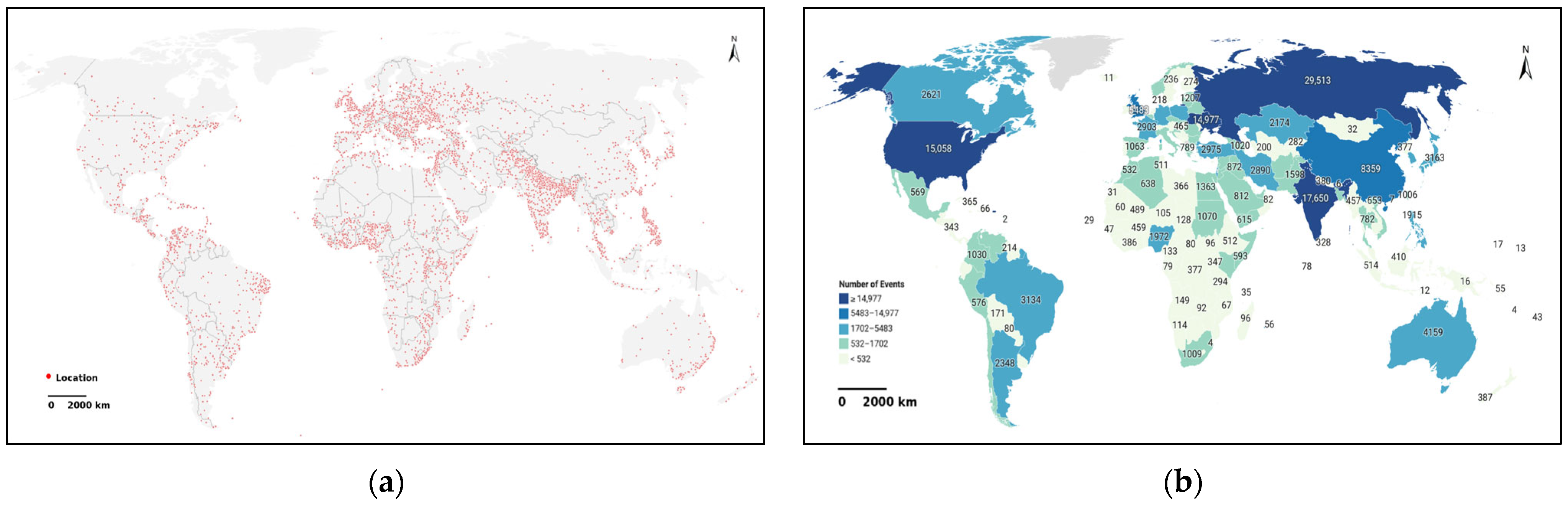
This study conducts a spatial analysis of the GDELT dataset by plotting all event coordinates and aggregating event counts at the national level, as shown in Figure 1.

Figure 1a illustrates the global distribution of event locations. Events are densely concentrated in highly urbanized and populous regions—such as Europe, East and South Asia, and the coastal areas of North America—forming clear spatial hotspots. In contrast, sparsely populated regions like Central Asia, the Sahara, and Antarctica record minimal events, reflecting the correlation between human activity intensity and event observability. Figure 1b visualizes the number of events per country, revealing marked regional disparities. Russia, India, the United States, and China rank highest in frequency due to their large populations and advanced media infrastructures. Middle Eastern countries such as Iraq and Syria also show high counts, driven by ongoing conflicts. Meanwhile, many countries in Africa, Central America, and the Pacific report very few events, potentially due to limited media coverage rather than low activity. Together, these figures reveal uneven global event visibility shaped by socio-political, technological, and observational factors.

The HAD dataset is constructed based on geographic divisions defined by China’s administrative hierarchy. It spans the administrative divisions from 1949 to 2019 and primarily consists of three levels: province, city, and county. It captures the structural evolution and jurisdictional changes of administrative divisions over the decades. HAD contains 216,695 triples, including 6454 geographic entities and an equal number of spatio-temporal records.

ICEWS is a comprehensive, integrated, automated, generalizable, and validated system designed to monitor, assess, and forecast national, sub-national, and internal crises. It consists of coded interactions between socio-political actors, including cooperative or hostile actions between individuals, groups, sectors, and nation-states. Events are automatically identified and extracted from news articles using the BBN ACCENT event coder. These events are represented as triples, consisting of a source actor, an event type (according to the CAMEO taxonomy of events), and a target actor. Geographical and temporal metadata are also extracted and associated with the relevant events within a news article. For this study, we used data from the ICEWS Coded Event Data from 2014. The dataset contains a total of 181,460 triples, including 7128 entities, 230 relations, and 181,460 spatio-temporal records.

A partial view of each dataset is illustrated in Figure 2. Then the dataset is divided into training, validation, and testing sets in a ratio of 90:1:9. The dataset partitioning details are shown in

Table 1. Dataset statistics of GDELT, ICEWS, and HAD.

	HAD			GDELT			ICEWS
	Training	Validation	Testing	Training	Validation	Testing	Training	Validation	Testing
Triple	195,025	2167	19,503	302,553	3362	20,255	163,314	1815	16,331
Relation	1	-	-	238	-	-	230	-	-
Entity	6454	-	-	6385	-	-	7128	-	-

.

2.2. ST-EKA

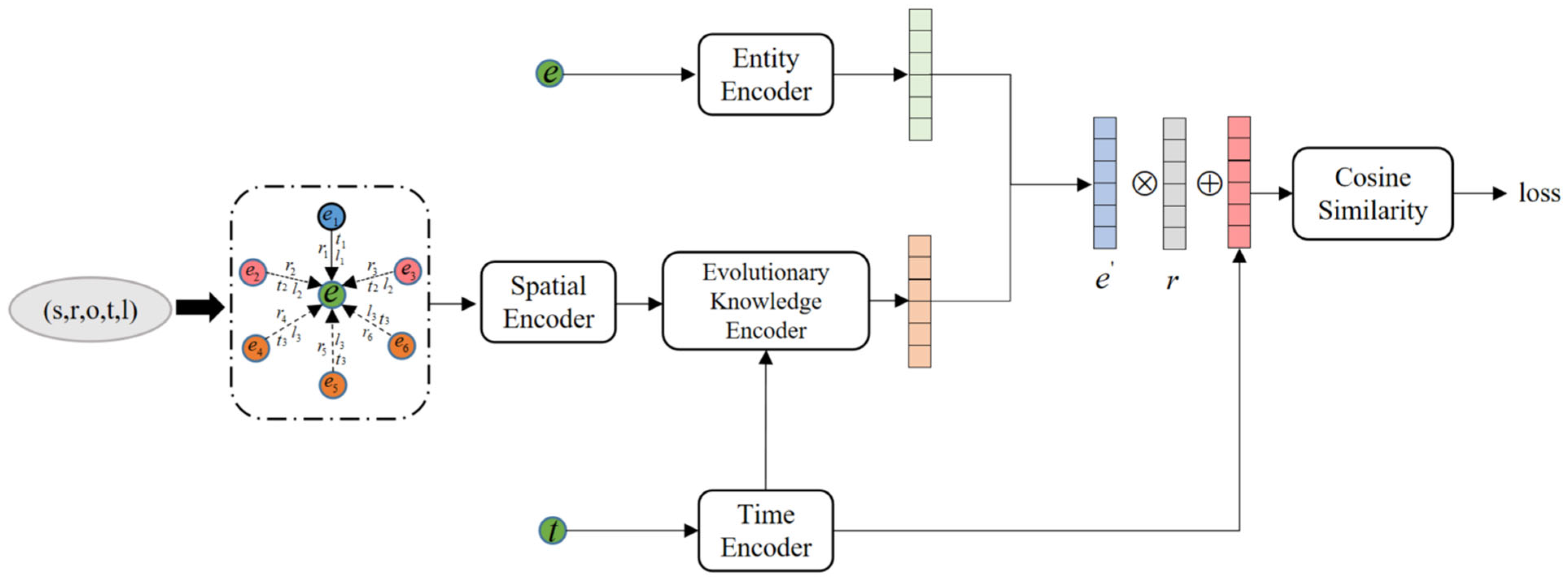
ST-EKA is designed to enhance entity representations by capturing their spatio-temporal evolution. The framework comprises four core components, as illustrated in Figure 3. The first component is the Entity Encoder. This module leverages the observation that entities connected by the same relation—either as head or tail—tend to share the same type. To model this property, we impose relation-specific similarity constraints and assign semantic types to each entity accordingly. We then employ entity-type matrices to generate embeddings, which are subsequently refined using relational constraints.

The second component is the Temporal Encoder. This module classifies temporal information in the knowledge graph into three categories: time points, time periods, and no time. Each category is processed separately to generate time-aware embeddings, thereby enabling precise temporal representation of entities. In temporal geographic knowledge graphs, however, the influence of neighboring nodes on a target entity is inherently time dependent. As entities and their relationships evolve over time, temporally proximate neighbors typically exert a greater influence, a phenomenon commonly referred to as the time decay effect. Traditional aggregation methods, which assign uniform or static weights to all neighbors regardless of their temporal distance, are inadequate for capturing such temporal dynamics. Consequently, these approaches often yield suboptimal representations for entities with evolving temporal contexts.

The third component is the Spatial Encoder. This module encodes spatial locations across multiple scales and takes into account the displacement relationships between different latitude–longitude coordinates. It then integrates these with the spatial attribute encodings associated with each coordinate to generate a comprehensive spatial representation. This enables the model to capture both fine-grained local spatial details and broader global spatial patterns, thereby enhancing its capacity to represent complex environmental contexts. Moreover, the influence of neighboring nodes on the target entity is spatially variant, exhibiting a distance-based attenuation effect—that is, the greater the spatial distance, the weaker the influence. This spatial decay mechanism reflects the intuition that proximity often correlates with stronger spatial relevance in real-world geospatial systems.

The fourth component is the Evolutionary Knowledge Encoder. To explicitly model the spatio-temporal decay effect, this module assigns corresponding weights to neighboring nodes based on their spatio-temporal proximity. Spatio-temporally closer neighbors receive greater weights, reflecting their stronger influence on the target entity’s current state. The encoder then aggregates the weighted neighboring quadruples to produce a neighborhood-level embedding. This captures the entity’s evolutionary characteristics, thereby enhancing its overall representation.

2.2.1. Entity Encoder

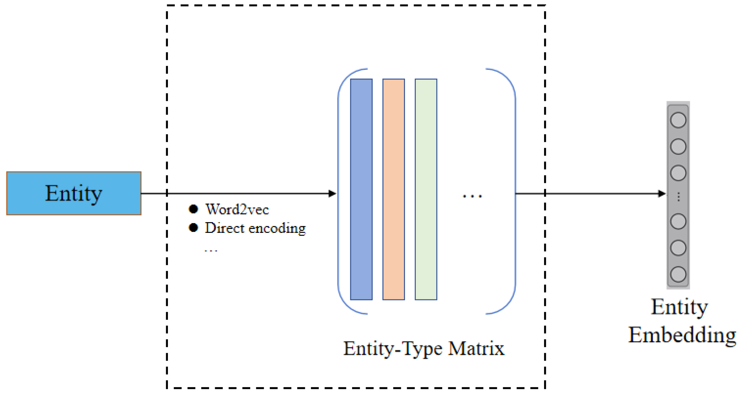
Typically, an entity encoder extracts key features of an entity and encodes them as high-dimensional vectors for subsequent processing in neural network modules. In traditional models, this step is commonly implemented using a randomly initialized embedding matrix. However, TaRP reveals that a substantial portion of information encoded in entity embeddings is inherently type-dependent. Based on this insight, we first classify entities according to the principle that head or tail entities connected by the same relation typically belong to the same type. We then employ an entity-type embedding matrix to encode entities of different types, thereby implicitly incorporating relational constraints. Each column of this matrix corresponds to a distinct entity type, as illustrated in Figure 4. We define the Entity Encoder Enc() as follows: Given any entity $e\in E$, where the type of e is $l_e\in L$, and L is the set of all entity types, the entity encoder proceeds as follows: First represents $e$ as a vector $w$. Next, perform an embedding lookup operation in the entity type embedding matrix $M$, where each column corresponds to a specific entity type. This retrieves the embedding of the entity’s type $M_{l_e}$. Multiply the entity embedding $w$ and the entity type embedding $M_{l_e}$ to combine the entity’s features with its type-specific features. Finally, normalize the result using the L2 norm to ensure consistency and scale invariance:

$$\epsilon =Enc(e)={\displaystyle \frac{M_{l_e}w}{\parallel M_{l_e}w{\parallel }_{L_2}}}$$

(1)

where $\mathsf{\epsilon }$ denotes the final entity feature embedding, $M_{l_e}$ is the entity type embedding matrix, $w$ is the entity’s encoding vector, and ${\parallel ·\parallel }_{L2}$ represents the L2 norm, which is the square root of the sum of the squared elements of vector.

2.2.2. Time Encoder

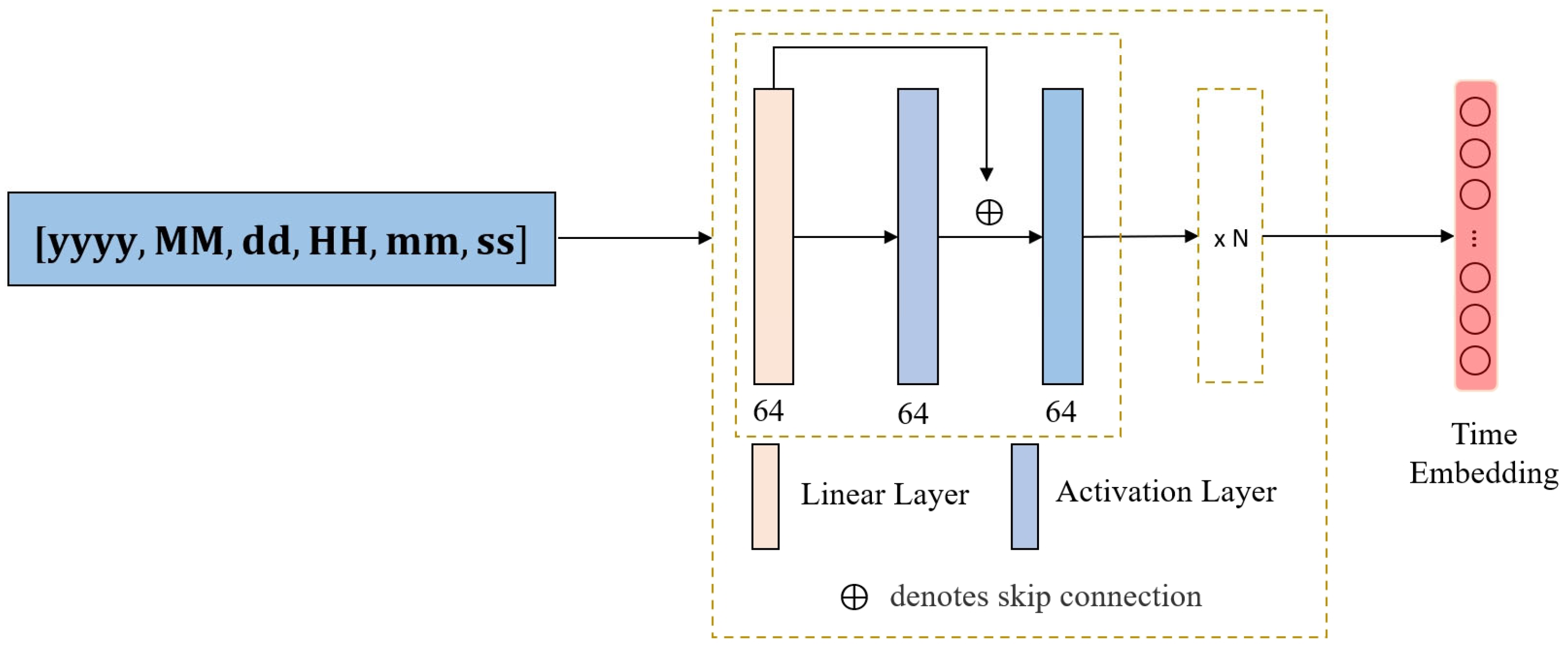
The time encoder is designed to express time as a high-dimensional vector, aiming to preserve both the scale information and temporal context, ensuring that no temporal information is lost. Most existing time encoders focus on a single time scalar, and here we also unify the representation of time. All times are unified into a 6-dimensional vector: $\mathrm{t}=[\mathrm{y}\mathrm{y}\mathrm{y}\mathrm{y},\mathrm{M}\mathrm{M},\mathrm{d}\mathrm{d},\mathrm{H}\mathrm{H},\mathrm{m}\mathrm{m},\mathrm{s}\mathrm{s}]$ representing year, month, day, hour, minute, and second, respectively. Due to the multiple recording forms of time in knowledge graphs, it is crucial for time encoders to be able to handle various types of time. Here we divide the time in the knowledge graph into the following three categories:

Time points $[t_1,t_2,\dots ,t_i]$: Some quadruples may possess multiple time points, such as (First District, is part of, Beijing City, [1949-10-01 00:00:00, 1950-10-01 00:00:00]). In such cases, we select one time point via uniform sampling. This approach ensures that all possible temporal information is eventually leveraged over multiple training steps.

Time period $[t_{min},t_{max}]$: For example, (1949-10-01 00:00:00, 1969-10-01 00:00:00). In the model, time intervals are converted to time points for computation. There are various conversion methods, such as using the start, end, or midpoint of the interval as the representative point. Methods that can convert time intervals to time points are generally applicable. However, to retain the scale information inherent in time intervals, simplistic methods like substituting intervals with only their start or end times are inadequate. Thus, similar to the handling of multiple time points, we use uniform sampling within the interval to select a time point.

No time $\mathrm{t}=\mathrm{\varnothing }$: For some quadruples, the time may be missing. In such cases, we assign the time range of the dataset to these quadruples. For instance, if the dataset represents a historical administrative division knowledge graph spanning from 1949-10-01 00:00:00 to 2023-10-01 00:00:00, then we use the interval [1949-10-01 00:00:00, 2023-10-01 00:00:00] as the time for these quadruples. This time interval is then processed in the same manner as other time intervals.

Through time classification and uniform sampling, the three types of time are converted into a single time point for processing. Then we use a feedforward neural network (FFN) encoder to encode the selected time point, generating a time embedding, as shown in Figure 5. Furthermore, through iterative training and dimensionality reduction sampling, the encoder is ensured to accurately encode all three types of time while preserving essential information.

$$\tau =T(t)=\left\{\begin{array}{ll}FFN(U([t_1,t_2,t_3,\cdots ,t_i]))& if t=[t_1,t_2,t_3,\cdots ,t_i]\\ FFN(U([t_{\min },t_{\max }]))& if t=[t_{\min },t_{\max }]\\ FFN(U([t_{start},t_{end}]))& if t=\varnothing \end{array}\right.$$

(2)

where $\tau$ represents time embedding, $U\left(\right)$ represents uniform sampling, $t_{start},t_{end}$ represent the start and end times of the dataset, FFN represents feedforward neural network encoding.

2.2.3. Spatial Encoder

This study designs a spatial encoder that combines Spatial Location and Spatial Attributes (LA). The spatial location is represented by geographic coordinates in the form of a two-dimensional vector $x=(lat,lon)$, where lat denotes latitude and lon denotes longitude. Each data point or entity corresponds to a two-dimensional (2D) spatial point $x$. The spatial attributes include address, city, country, sea area, point of interest (POI), land use type, etc.

(1)

Spatial Location Encoder

This study proposes a multi-scale spatial location encoder. For any given 2D spatial point $x$, sine and cosine functions with different frequencies are used to encode the coordinate value:

$${\rho }_l=En{c}_{pos}(x)=NN(P{E}^{(t)}(x))$$

(3)

where ${\mathrm{PE}}^{(t)}(x)=[{\mathrm{PE}}_0^{(t)}(x);\cdots ;{\mathrm{PE}}_s^{(t)}(x);\cdots ;{\mathrm{PE}}_{S-1}^{(t)}(x)]$ represents the concatenation of multi-scale encodings. The dimensionality of $PE\left(x\right)$ is $6S$, where $S$ denotes the total number of scales, with $s=0,1,2,\cdots ,S-1$. The function $NN(·)$ denotes a fully connected ReLU layer.

Then, three two-dimensional unit vectors are defined:

$${\alpha }_1=\left[\begin{array}{l}1\\ 0\end{array}\right],{\alpha }_2=\left[\begin{array}{l}-{\displaystyle \frac{1}{2}}\\ {\displaystyle \frac{\sqrt{3}}{2}}\end{array}\right],{\alpha }_3=\left[\begin{array}{l}-{\displaystyle \frac{1}{2}}\\ -{\displaystyle \frac{\sqrt{3}}{2}}\end{array}\right]\in {ℝ}^2$$

(4)

where ${\alpha }_1,{\alpha }_2,{\alpha }_3$ are three unit vectors with equal angular spacing of ${\displaystyle \frac{2\pi }{3}}$.

At each scale $s$, the positional encoding $P{E}_s^{(t)}(x)$ is defined as:

$$P{E}_s^{(t)}(x)=[P{E}_{s,1}^{(t)}(x);P{E}_{s,2}^{(t)}(x);P{E}_{s,3}^{(t)}(x)]$$

(5)

where

$$P{E}_{s,j}^{(t)}(x)=\left[\begin{array}{l}\cos ({\displaystyle \frac{<x,{\alpha }_j>}{{\lambda }_{\min }·g^{s/(S-1)}}})\\ \sin ({\displaystyle \frac{<x,{\alpha }_j>}{{\lambda }_{\min }·g^{s/(S-1)}}})\end{array}\right],\forall j=1,2,3$$

(6)

Here, ${\lambda }_{\min }$ and ${\lambda }_{\max }$ denote the minimum and maximum wavelength scales, and $g={\lambda }_{\max }/{\lambda }_{\min }$ controls the scale range. A larger value of $g$ indicates a broader range of scale encoding, allowing the model to perform encoding at more extensive spatial levels. Through this encoding mechanism, the model can simultaneously capture fine-grained local spatial structures and broader global spatial information, thereby enhancing its capability to represent complex spatial distributions.

To ensure translation invariance, the following condition must be satisfied:

$$En{c}_{pos}(x+\Delta x)=M(\Delta x)En{c}_{pos}(x)$$

(7)

where $\Delta x$ represents the displacement in the 2D spatial domain, and the matrix $M(\Delta x)$ performs rotation and translation operations to achieve position updates. $C^{\ast }C=I$, where $I$ is the identity matrix.

(2)

Spatial Attribute Encoder

After completing the spatial location embedding, the corresponding spatial attributes such as address, city, country, sea area, point of interest (POI), and land use type are encoded using Word2Vec. These spatial attribute embeddings are concatenated with the position encoding and passed through a linear transformation to obtain the final spatial feature vector, as shown in Figure 6.

$$\rho =Linear({\rho }_l\oplus \underset{\mathrm{multivariable}: \left[x,y,\cdots ,z\right]}{\underbrace{W2V(x)\oplus W2V(y)\oplus \cdots \oplus W2V(z)}})$$

(8)

Here, $W2V$ denotes the Word2Vec embedding of the spatial attribute values x, y, …, z; $\oplus$ represents vector concatenation; and $\mathrm{L}\mathrm{i}\mathrm{n}\mathrm{e}\mathrm{a}\mathrm{r}\left(\right)$ is a fully connected linear transformation layer.

2.2.4. Evolutionary Knowledge Encoder

Considering the spatio-temporal decay effect, we hypothesize that the spatio-temporal proximity between adjacent entities significantly affects the influence exerted by its neighboring nodes. Specifically, the closer the spatio-temporal proximity, the greater the influence of neighboring nodes on the entity [44,45,46,47].

Firstly, adjacent quadruples are categorized into two types based on the position of the target entity within the quadruple:

(1)

When the target entity appears as the tail entity, the corresponding quadruple is regarded as part of the formation process of the entity. For example, in the quadruple (Continuous heavy rainfall, caused, 18 March 2025, 4:50 a.m., Fugong landslide), “Fugong landslide” is the target entity, and “continuous heavy rainfall” is the inducing factor.

(2)

When the target entity appears as the head entity, the corresponding quadruple reflects the consequences or impact exerted by the entity on other entities. For instance, in (Fugong landslide, caused, 18 March 2025, 4:50 a.m., 1 dead and 4 missing), “Fugong landslide” is the target entity, and “1 dead and 4 missing” represents the resulting impact.

These two types of quadruples jointly reveal the spatio-temporal evolution trajectory of the target entity within the knowledge graph. However, directly modeling both types of relationships would significantly increase the computational and modeling complexity.

To simplify the algorithm, reverse relations are added for all existing relations, and the corresponding quadruples are inverted. This transformation simplifies the problem by focusing only on quadruples in which the entity serves as the tail. The attention mechanism [48] is then applied to calculate the weights for the time embedding and spatial embedding.

$$w=Softmax({\displaystyle \frac{Q·K^T}{\sqrt{d_k}}})·V$$

(9)

where Q, K, and V are the query, key, and value matrices generated by linear layers for each adjacent quadruple time embedding, and d_k is the dimension.

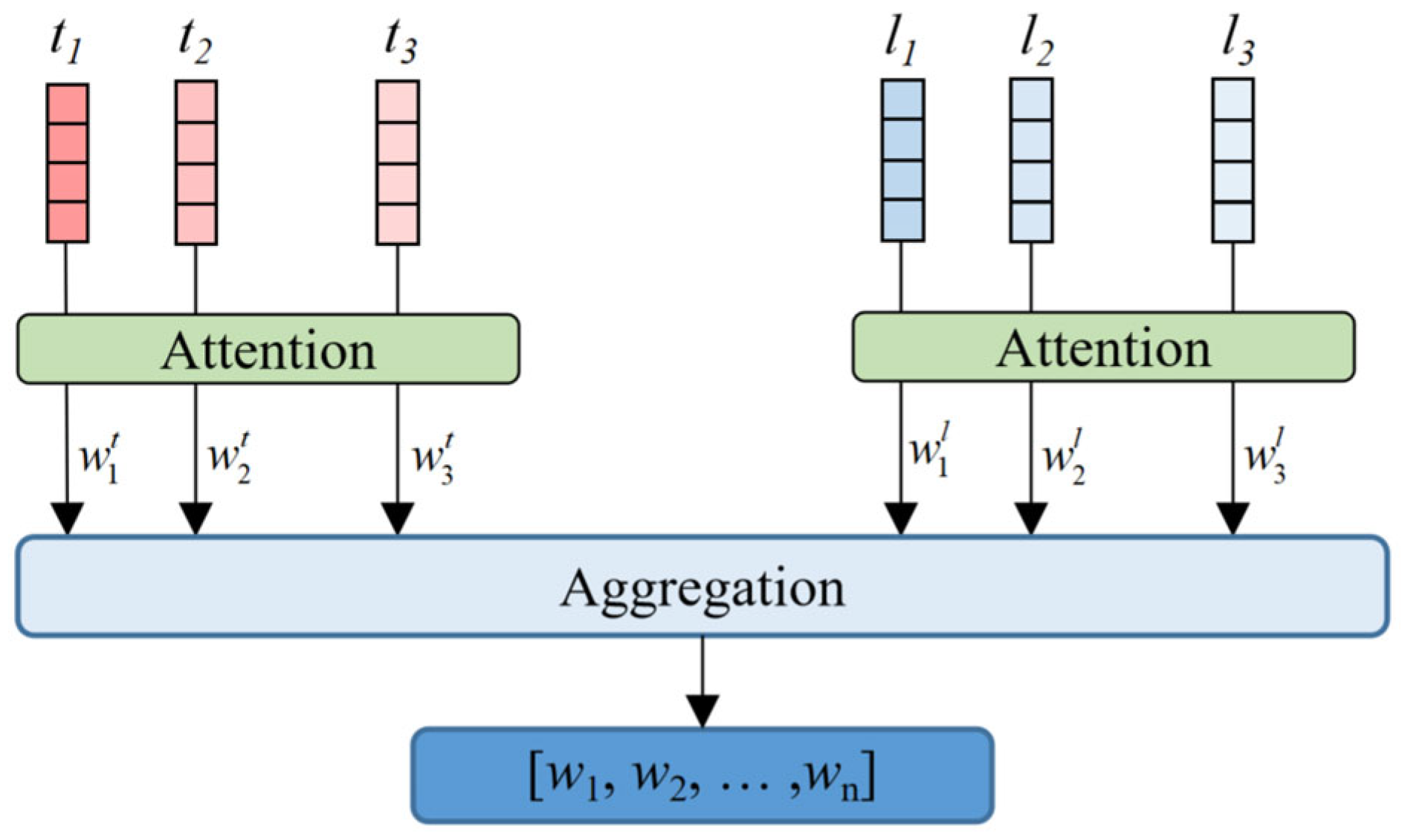
Subsequently, the spatial and temporal weights are aggregated to obtain an integrated spatio-temporal weight, as illustrated in Figure 7. Then, for each adjacent quadruple, the embedding is computed based on the embedding of the neighboring node, the corresponding relation, and the spatio-temporal weight assigned to the group to which the quadruple belongs:

$${\epsilon }^{\prime }=\epsilon \otimes R_r\otimes (w_t\otimes w_l)$$

(10)

where $\epsilon$ denotes the neighboring entity, and $R_r$ denotes the relation corresponding to the neighboring entity.

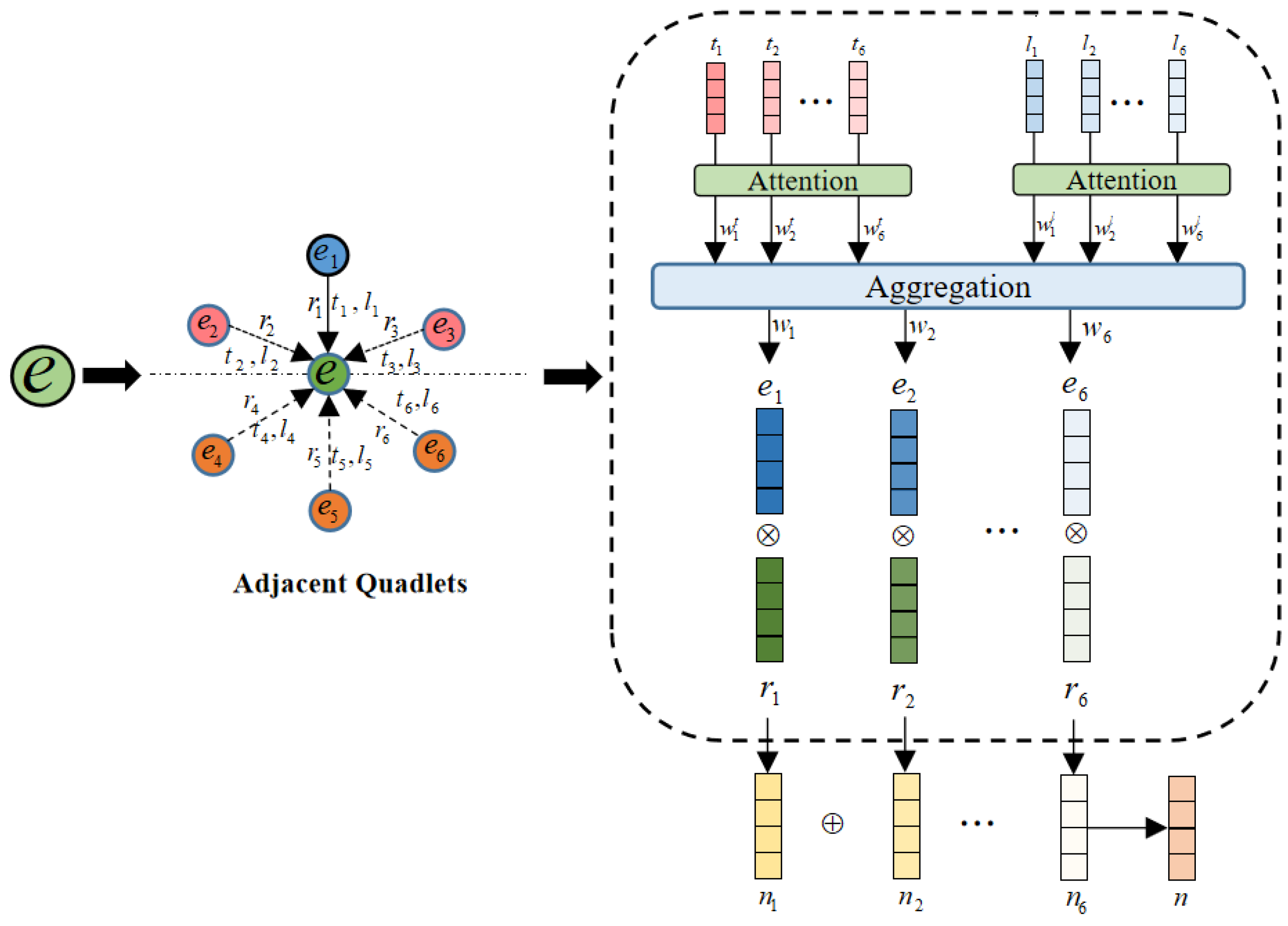
After performing the above calculation on all adjacent quadruples, the encodings of all adjacent quadruples are aggregated to obtain the neighborhood information of the entity, as shown in Figure 8:

$$nei={\displaystyle \sum _{i=1}^m{\epsilon }_i\otimes R_{r_i}\otimes w_i}$$

(11)

where ${\epsilon }_i$ represents the encoding of adjacent node, $R_{r_i}$ represents the relationship between adjacent node and target node, $w_i$ is the corresponding spatio-temporal weight, and m is the number of adjacent nodes.

Finally, we fuse neighborhood information with entity embedding to obtain a spatio-temporal evolutionary knowledge aware entity enhanced representation, and calculate it with relationship and time to obtain the predict tail entity embedding, denoted as $\mathsf{\sigma }$:

$$\sigma =(nei+{\epsilon }_{\mathrm{h}})\otimes R_r+\tau$$

(12)

where $nei$ represents the entity spatio-temporal evolution embedding, ${\epsilon }_h$ represents the head entity embedding, $\mathsf{\tau }$ represents the time embedding.

We then use the cosine similarity function to calculate the loss values between $\mathsf{\sigma }$ and both the positive and negative samples, and obtain the final loss value:

$$cos\left(e_1,e_2\right)={\displaystyle \frac{e_1{e}_2}{\parallel e_1\parallel \parallel e_2\parallel }}$$

(13)

$$loss=1-(\cos (\sigma ,{\epsilon }_o)-\cos (\sigma ,{\epsilon }_{neg}))$$

(14)

where ${\mathsf{\epsilon }}_o$ represents the positive tail entity embedding, and ${\mathsf{\epsilon }}_{neg}$ represents the negative tail entity embedding.

The training objective is to minimize the distance between the predicted embedding and the correct entity embedding, while maximizing the gap with the negative samples. In other words, the goal is to make $\cos (\sigma ,{\epsilon }_o)$ as close to 1 as possible, $\cos (\sigma ,{\epsilon }_{neg})$ as close to 0 as possible, and ultimately minimize loss to approach 0.

2.3. Question-Answering Model

We further evaluate the performance of ST-EKA on the question answering (Q&A) task. Graph query embedding (GQE) is an end-to-end logical query answering model designed to handle connected graph queries [49]. Contextual graph attention (CGA) extends GQE by integrating a self-attention-based intersection operator [50]. In this study, we adopt these two models as baselines and integrate ST-EKA into their architectures.

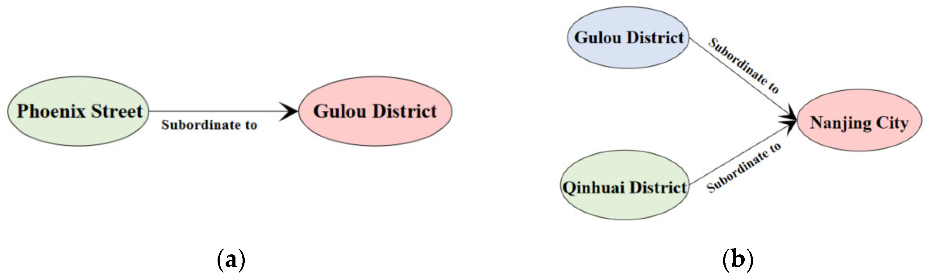
In Q&A tasks, any complex query graph (QG) can be decomposed into a combination of chain and intersection structures. The chain structure is depicted in Figure 9a, whereas the intersection structure is illustrated in Figure 9b. As illustrated, the chain structure involves the processing of simple quadruples, for which ST-EKA is applied. In contrast, the intersection structure aggregates the outputs of several sub-query graphs to produce a combined result. To perform this operation, we retain the original intersection operator from the baseline models. We designed six types of QGs and conducted Q&A experiments based on these structures, incorporating both ST-EKA and the baseline intersection operators. A detailed introduction to the query graphs is provided in Section 3.3.

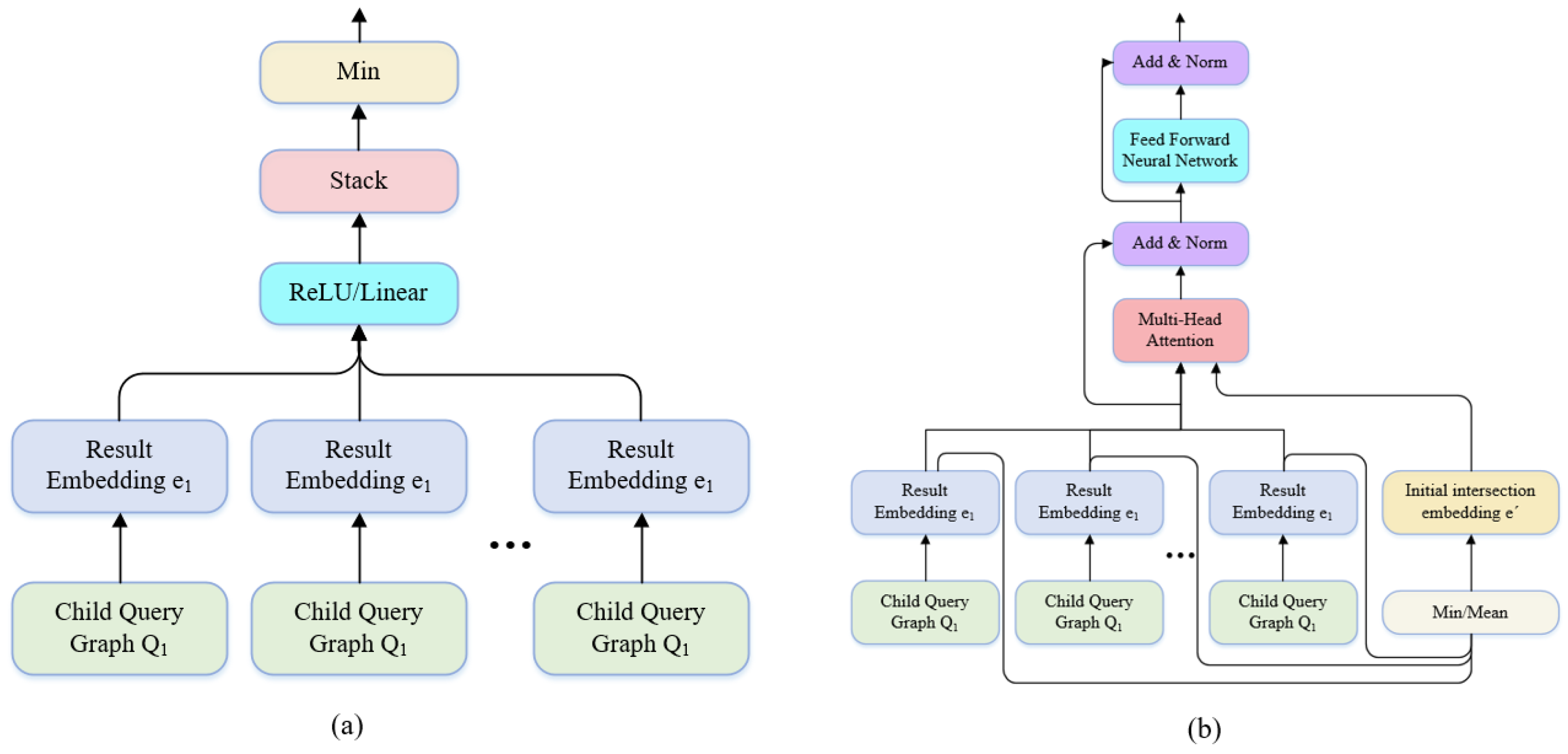
The intersection operator is used to consolidate multiple vectors into a single vector. Typically, any method that preserves the original sequence of input vectors, such as taking the minimum, maximum, or average, is applicable. The GQE model utilizes a linear feedforward network combined with a minimum function as the intersection operator, as shown in Figure 10a. The CGA model improves this intersection operator by incorporating a self-attention mechanism, as shown in Figure 10b.

When equipped with these two basic neural network modules, any complex query graph can be encoded according to its structure to obtain a unique result vector. This vector is then used to retrieve the most probable answer through nearest neighbor search in the entity space.

2.4. Model Training

2.4.1. Experimental Platform Configuration

The experiments in this study were conducted on a system equipped with an 11th Gen Intel (R) Core (TM) i9-11900K CPU @ 3.50 GHz, an NVIDIA GeForce RTX 3080 Ti GPU with 28 GB of memory, and 32 GB of RAM. The entire experiment was performed in a Windows environment. The implementation was based on Python 3.9 and PyTorch 1.12.1.

2.4.2. Model Parameter Settings

To mitigate overfitting, both the representation learning and question-answering tasks employ an early stopping strategy based on a predefined tolerance threshold. When the performance improvement falls below this threshold, the model is considered to have converged, and training is terminated early. The learning rate, which controls the step size for updating model parameters, has a critical impact on model performance. An excessively large learning rate may result in unstable loss fluctuations, whereas an overly small rate may lead to slow convergence. In our experiments, we tested multiple learning rates and observed that the optimal performance was achieved with a learning rate of 0.001 in combination with the Adam optimizer. This training configuration ensures both computational efficiency and high model performance. The detailed hyper parameter settings for each model are summarized in

Table 2. Hyper parameter settings.

Parameter	ST-EKA	GQE	CGA
Entity embedding dimension	64	64	64
Time encoder	FFN	FFN	FFN
Spatial encoder	LA	LA	LA
Time embedding dimension	64	64	64
Learning rate	0.001	0.001	0.001
Activation function	LeakyReLU	LeakyReLU	LeakyReLU
Time activation function	Sigmoid	Sigmoid	Sigmoid
Optimizer	Adam	Adam	Adam
Batch size	2048	2048	2048
Max training epochs	100,000	100,000	100,000
Tolerance threshold	1.00 × 10−6	1.00 × 10−6	1.00 × 10−6
Decoder	-	Bilinear	Bilinear
Intersection operator	-	Minimum	Minimum (self-attention)

.

2.4.3. Training Phase

The training of the Q&A model consists of the intrinsic structure of the KG and a series of query-answer pairs. The final loss function is defined as follows:

$$L=L_{KG}+L_{QA}$$

(15)

(1)

KG Training Phase

During the KG training phase, we treat the quadruples in the KG as the basis chain query graph, predicting the tail entity using ST-EKA. The purpose of this step is to pre-train the model and obtain embeddings for entities, relationships, and time:

$$L_{KG}={\displaystyle \sum _{i=1}^n\max (0,1-\left[cos\left(e_i^p,e_i^o\right)-cos\left(e_i^p,e_i^n\right)\right]})$$

(16)

where $e_i^p$ represents the predicted result, $e_i^o$ represents the tail entity, and $e_i^n$ represents the negative sample.

(2)

Question-Answer Pair Training Phase

We design six types of query graphs, and sample each type to obtain question-answer pairs in the form of $(Q,A,Neg)$, where $Q$ represents the question with a different query graph type, $A$ represents the correct answer, and $Neg$ represents the incorrect answer, i.e., the negative sample. The sampling method first sorts the nodes within the query graph according to their topological sequence and then performs the sampling based on this order, selecting one basic graph structure at a time. The training objective is to minimize the distance between the predicted embedding and the correct entity embedding while maximizing the gap with the negative samples. Cosine similarity is chosen as the method to compute the similarity:

$$L_{QA}={\displaystyle \sum _{q_i,a_i\in \chi }{\displaystyle \sum _{i=1}^X}\max (0,1-\left[\omega (\psi ({\mathrm{Q}}_i),A_i)-\omega (\psi ({\mathrm{Q}}_i),Ne{g}_i)\right]})$$

(17)

where $\psi ()$ represents the function that calculates the predicted result based on the query graph structure, and $a_n$ signifies the negative sample.

3. Results and Discussion

Model performance is evaluated using two metrics: area under the receiver operating characteristic curve (AUC) and average percentile rank (APR). AUC quantifies the model’s ability to distinguish correct answers from negative samples by computing the area under the ROC curve, which reflects the trade-off between true positive and false positive rates. A higher AUC value (closer to 1) indicates stronger discriminative capability. APR measures the average percentile position of the correct answer among all predicted candidates. It reflects how effectively the model ranks correct answers relative to negative ones—higher APR values indicate better ranking performance.

3.1. Comparison Between ST-EKA and Other Representation Learning Methods

We selected five state-of-the-art (SOTA) methods for comparison: TransE, TTransE, TeRo, HyTE, and TeAST. ST-EKA aggregates adjacent node information, but in a knowledge graph, the number of neighbors of a node can vary significantly—some nodes have only one neighbor, while others may have thousands. When there is a large number of neighboring nodes, considering all of them becomes inefficient. Therefore, it is necessary to sample the neighboring nodes; we base our sampling strategy on time. Specifically, we first sort the quadruples with the target entity as the tail entity by time and select the three quadruples with the largest time as the causal quadruples. For quadruples with the target entity as the head entity, we select the three quadruples with the smallest time as result quadruples. These six quadruples are then used as neighboring quadruples for training. After sampling, ST-EKA is applied for training. The experimental results are shown in

Table 3. The results of ST-EKA and SOTA methods.

Dataset	TransE		TTransE		TeRo		HyTE		TeAST		ST-EKA
	AUC	APR	AUC	APR	AUC	APR	AUC	APR	AUC	APR	AUC	APR
GDELT	0.902518	91.4722	0.942230	94.2445	0.929424	92.5342	0.944124	94.8394	0.921868	93.8762	0.949833	95.3718
HAD	0.641902	67.0304	0.671307	72.9373	0.608022	61.1551	0.669956	69.6370	0.672938	66.2046	0.782160	76.7154
ICEWS	0.830457	85.3953	0.902596	90.4274	0.924264	91.8489	0.933134	92.9304	0.916625	91.9483	0.947602	94.5066

.

From Table 3, it can be observed that ST-EKA achieves the highest AUC and APR scores across all datasets, with the most notable improvement on the GDELT dataset. Compared with baseline methods, ST-EKA improves AUC by 4.7315% over TransE, 0.7603% over TTransE, 2.0409% over TeRo, 0.5709% over HyTE, and 2.7965% over TeAST. Unlike entity-centric knowledge graphs, GDELT focuses on dynamic international events, where temporal progression and evolving relationships among geopolitical actors are essential for understanding event causality and influence chains. ST-EKA effectively models these dynamics by incorporating both the temporal decay of neighboring quadruples and type-aware entity constraints. This results in more accurate and context-rich event embeddings, which are critical for downstream geographic question-answering tasks that require fine-grained temporal inference.

On HAD, ST-EKA improves AUC by 14.0258% over TransE, 11.0853% over TTransE, 17.4138% over TeRo, 11.2204% over HyTE, and 10.9222% over TeAST. On ICEWS, ST-EKA outperforms TransE by 11.7145%, as well as achieving respective gains of 11.7145%, 4.5006%, 2.3338%, 1.4468%, and 3.0977% over other methods. These results confirm that the spatio-temporal evolutionary embedding mechanism introduced in ST-EKA can be effectively generalized to different domains, including structured administrative knowledge (HAD) and socio-political event streams (ICEWS).

Based on the results from all three datasets, ST-EKA effectively improves representation learning by assigning types to entities through relationships, enhancing entity representation with relationship constraints, and incorporating weights based on the temporal dynamics of quadruples. These strategies allow ST-EKA to capture entity evolution knowledge and further refine the entity representation. Overall, ST-EKA is shown to be both effective and efficient.

3.2. Ablation Study

To evaluate the contribution of each component in ST-EKA, we conducted ablation experiments on the HAD, GDELT, and ICEWS datasets. The following model variants were assessed:

(1)

w/o TimeDecay: This variant removes the temporal weighting module from the evolutionary knowledge encoder and uses only spatial weight for aggregation.

(2)

w/o SpatialDecay: This variant removes the spatial weighting module from the evolutionary knowledge encoder and uses only temporal weight for aggregation.

(3)

w/o Evolutionary Knowledge Encoder: This variant eliminates the entire evolutionary knowledge encoder module.

(4)

Number of adjacent quadruples: This setting tests the effect of varying the number of adjacent quadruples used in the evolutionary knowledge encoder. The sampling strategy for adjacent quadruples is described in Section 3.1.

It is important to note that, unless otherwise specified, the number of adjacent quadruples used in other experiments, including the w/o TimeDecay variant and the w/o SpatialDecay, is fixed at 6. The experimental results are summarized in

Table 4. Ablation results on GDELT, HAD, and ICEWS datasets.

Variant		GDELT		HAD		ICEWS
		AUC	APR	AUC	APR	AUC	APR
w/o TimeDecay		0.931227	93.9201	0.601407	60.6120	0.912682	90.8126
w/o SpatialDecay		0.940203	94.1862	0.607226	60.1973	0.902509	90.2744
w/o Evolutionary Knowledge Encoder		0.929124	92.0958	0.455195	45.8746	0.907948	89.7972
Number of adjacent quadruples	2	0.937942	94.1132	0.706877	70.9604	0.935176	93.4767
	4	0.938235	94.2296	0.748483	72.9411	0.936799	93.9902
	6	0.949833	95.3718	0.782160	76.7154	0.947602	94.5066
	8	0.947735	94.5333	0.805438	81.1896	0.950262	94.6585

.

As shown in Table 4, removing the temporal weight (w/o TimeDecay) leads to performance degradation across all datasets. On the GDELT dataset, the AUC drops from 0.949833 to 0.931227, suggesting that using only spatial weight to aggregate neighboring quadruples fails to capture their dynamic temporal correlations, thereby neglecting the time decay effect. In addition, the ablation of the spatial weight (w/o SpatialDecay) also leads to a performance drop, with the AUC decreasing to 0.940203, demonstrating that neglecting temporal proximity similarly weakens the model’s ability to capture contextual influence—especially in event-centric graphs where temporal plays a critical role. The performance decline is even more pronounced on the HAD dataset. Removing the time decay mechanism results in an AUC drop from 0.782160 to 0.601407, and eliminating the spatial decay module reduces it to 0.607226, reflecting relative decreases of 18.0753% and 17.4934%, respectively. Moreover, removing the evolutionary knowledge encoder results in the most significant performance decline—specifically, a drop of 2.0709% in AUC on the GDELT dataset, 32.6965% on the HAD dataset, and 3.9654% on the ICEWS dataset. This highlights the indispensable role of entity evolutionary knowledge in handling diverse and heterogeneous datasets.

Meanwhile, as the number of adjacent quadruples used by the evolutionary knowledge encoder increases, the model performance steadily improves. On GDELT, the AUC grows from 0.937942 (2 quadruples) to 0.949833 (6 quadruples) and remains high at 0.947735 with 8 quadruples. Similar patterns are observed on HAD and ICEWS, affirming that richer spatio-temporal context enhances representation learning. These results collectively confirm the effectiveness of the proposed temporal and spatial weighting mechanisms and the evolutionary knowledge encoder in capturing spatio-temporal entity evolution for event-based reasoning tasks.

3.3. Application of ST-EKA in Geographic Knowledge Graph Question-Answering Tasks

After confirming ST-EKA’s strong performance in representation learning, we focused on its application to downstream query question answering tasks. In this experiment, we designed six types of query graphs for the Q&A task, as shown in Figure 11:

2-inter: Intersection structure formed by two quadruples whose tail entities are connected.

2-chain: A chain structure composed sequentially of two quadruples’ head and tail entities.

3-chain_inter: Formed by connecting the tail node of a 2-inter structure to another quadruple.

3-inter_chain: Formed by connecting the tail node of a 2-chain structure to another quadruple.

3-inter: Intersection structure formed by three quadruples whose tail entities are connected.

3-chain: A chain structure composed sequentially of three quadruples’ head and tail entities.

We first conducted question–answer sampling based on these six query graphs. The training QAs must have answers derived from the training set, meaning the training QAs are sampled based on the training quadruple set. In contrast, validation and test QAs are sampled from the entire dataset. Specifically, each QA in the validation and test sets contains at least one quadruple not present in the training set. The number of QAs is shown in

Table 5. QA statistics of GDELT, HAD, and ICEWS.

QG Type	GDELT			HAD			ICEWS
	Training	Validation	Testing	Training	Validation	Testing	Training	Validation	Testing
2-inter	496,603	898	9000	427,235	726	10,000	451,184	861	9000
2-chain	503,397	899	9000	572,765	778	10,000	548,816	866	9000
3-chain_inter	248,437	900	9000	235,880	861	10,000	196,861	895	9000
3-inter_chain	250,046	900	9000	241,778	834	10,000	256,982	897	9000
3-inter	249,753	899	9000	215,893	930	10,000	256,787	890	9000
3-chain	251,764	899	9000	306,449	632	10,000	289,370	896	9000

.

We selected two baseline models, CGA and GQE, and conducted comparative experiments by replacing the chain structure encoder in the original models with ST-EKA. This allowed us to assess how ST-EKA’s entity evolution modeling could improve the performance of these existing query answering frameworks. The experimental results are shown in

Table 6. Experimental results on GDELT dataset.

QG Type	GQE		GQE(ST-EKA)		CGA		CGA(ST-EKA)
	AUC	APR	AUC	APR	AUC	APR	AUC	APR
2-chain	0.843350	87.6403	0.882130	88.5873	0.847743	87.9664	0.891991	85.5697
2-inter	0.938444	93.9272	0.940005	93.5556	0.850209	82.2025	0.855429	82.4082
3-chain	0.804374	83.8110	0.851808	85.8270	0.811997	84.0545	0.871357	83.2847
3-inter	0.938924	94.3070	0.939747	94.0133	0.799320	78.1630	0.853859	82.2146
3-inter_chain	0.919941	90.9682	0.922091	90.0921	0.849684	81.8414	0.892362	84.9798
3-chain_inter	0.948497	95.0101	0.949520	94.6802	0.944780	94.7102	0.947833	94.3688
Macro averaged	0.898922	90.9440	0.914217	91.1259	0.850622	84.8230	0.885472	85.4710

,

Table 7. Experimental results on HAD dataset.

QG Type	GQE		GQE(ST-EKA)		CGA		CGA(ST-EKA)
	AUC	APR	AUC	APR	AUC	APR	AUC	APR
2-chain	0.961604	96.8974	0.968933	97.2518	0.965489	96.5949	0.977246	98.0323
2-inter	0.993087	99.5815	0.999189	99.6248	0.995919	99.7230	0.998415	99.6852
3-chain	0.955031	95.8342	0.963152	95.9083	0.952445	95.9101	0.964101	96.7924
3-inter	0.995193	99.6941	0.998470	99.8255	0.997673	99.8560	0.998146	99.8247
3-inter_chain	0.992001	99.2988	0.997943	99.5414	0.995748	99.6145	0.996948	99.5857
3-chain_inter	0.990952	99.1825	0.995659	99.2919	0.991282	99.2800	0.995122	99.3061
Macro averaged	0.981311	98.4148	0.987224	98.5740	0.983093	98.4964	0.988330	98.8711

and

Table 8. Experimental results on ICEWS dataset.

QG Type	GQE		GQE(ST-EKA)		CGA		CGA(ST-EKA)
	AUC	APR	AUC	APR	AUC	APR	AUC	APR
2-chain	0.918172	91.2901	0.937041	93.1939	0.917873	91.5223	0.939495	93.5107
2-inter	0.974377	97.4357	0.982674	97.8518	0.979914	98.3056	0.983228	98.3321
3-chain	0.886607	88.1777	0.916702	89.8376	0.886998	88.0748	0.920587	88.8951
3-inter	0.981251	98.5451	0.985191	98.5942	0.986658	98.7870	0.988850	98.9267
3-inter_chain	0.965495	96.3394	0.975739	96.7699	0.964760	96.0015	0.977448	97.3817
3-chain_inter	0.962303	96.6072	0.965868	96.8457	0.957734	96.0999	0.966128	96.1264
Macro averaged	0.948034	94.7325	0.960536	95.5155	0.948990	94.7985	0.962623	95.5288

.

As shown in Table 6, Table 7 and Table 8, the proposed ST-EKA model significantly improves the performance of geographic question-answering tasks. Among the three datasets, the GDELT dataset serves as the most representative benchmark due to its high event density, global scope, and fine-grained temporal granularity. In this context, ST-EKA demonstrates substantial improvements across all QG types. Taking the GDELT dataset as the main case, when integrated with the GQE model, ST-EKA improves the macro-averaged AUC by 1.5295% and APR by 0.1819. Based on the CGA model, the AUC increases by 3.4850% and the APR by 0.6480. These results confirm that the addition of ST-EKA effectively improves the overall query accuracy of the model.

Notably, ST-EKA explicitly models entity evolution by aggregating neighboring quadruples based on both temporal and spatial distances. Unlike prior methods that treat adjacent entities equally or rely solely on time-aware aggregation, ST-EKA introduces a dual-decay mechanism that assigns dynamic attention weights according to both time proximity and spatial proximity. This enables the model to capture not only temporal dependencies but also geographic co-occurrence patterns, leading to higher-quality event embeddings. Such fine-grained representation is particularly beneficial in geographic reasoning tasks, where the influence of nearby events is often subject to both spatial and temporal attenuation.

For chain-based query structures such as 2-chain and 3-chain, the improvements are even more significant—demonstrating that ST-EKA excels at sequential reasoning by capturing the progressive evolution of entities across space and time. For instance, in the GDELT dataset, the AUC improvement for the 3-chain QG under GQE reaches 4.7434%.

As shown in Figure 12, although ST-EKA also improves intersection-based QGs, the margin is relatively smaller—especially in the CGA backbone—where existing attention-based intersection operators already handle complex queries effectively. In fact, as observed in both the GDELT and HAD datasets, when the query structure contains intersection components, the intersection processors could not effectively integrate the evolutionary knowledge of entities, leading to less improvement or even a slight decrease in query accuracy. This suggests the need to redesign and optimize the intersection operator to better leverage the spatio-temporal embeddings produced by ST-EKA.

In HAD, which contains structured historical administrative changes, ST-EKA improves the GQE model’s macro AUC and APR by 0.5913% and 0.1592, respectively. In the ICEWS dataset—a temporal event dataset with clear geopolitical framing—macro AUC and APR improvements reach 1.2502% and 0.7830 under GQE, and 1.3633% and 0.7303 under CGA, respectively. These results underscore the adaptability of ST-EKA to various temporal and spatial resolutions and its strong capacity for generalization across different event types and spatial scales.

In summary, the integration of temporal and spatial decay mechanisms empowers ST-EKA to capture both temporal correlations and spatial influences, providing a more realistic and nuanced view of entity evolution. This design is especially valuable in geographic knowledge graphs, where entities often exhibit strong spatio-temporal clustering. By enhancing the quality of entity embeddings, ST-EKA not only boosts question answering accuracy but also sets a foundation for more interpretable and context-aware reasoning in spatio-temporal domains.

4. Discussion

In this study, we propose ST-EKA, a spatio-temporal evolutionary knowledge embedding approach, as a foundational representation learning model designed for geographic knowledge graph Q&A. Unlike traditional methods that primarily focus on structural information from static triples, ST-EKA captures the dynamic nature of entities by aggregating temporally and spatially adjacent quadruples. Through this fusion of temporal and spatial contexts, ST-EKA forms a structured representation of entity evolution, enhancing the expressiveness of embeddings for downstream tasks.

ST-EKA first categorizes temporal information in the GeoKG into distinct types and applies corresponding encoding strategies. Then, to overcome the neglect of spatio-temporal decay in neighbor aggregation, ST-EKA introduces an evolutionary knowledge encoder that divides neighboring quadruples into process-oriented and result-oriented types based on the head/tail role of the target entity. By assigning attention weights that decay with both temporal and spatial distance, the model emphasizes contextually relevant events and attenuates distant noise. Meanwhile, ontological features are enhanced by entity-type constraints. By integrating both spatio-temporal evolution and type-aware semantic information, the model produces enriched embeddings capable of capturing complex real-world transformations.

To verify the effectiveness of ST-EKA, we conducted comparative experiments against five state-of-the-art representation models on three representative datasets. Results in Table 3 confirm that ST-EKA performs particularly well in dynamic environments with rich spatio-temporal correlations, such as the GDELT and ICEWS datasets. On these datasets, where events exhibit both frequent temporal changes and broad geographic diversity, ST-EKA consistently outperforms the baseline models. In contrast, on the simpler HAD dataset, where variability is lower, models tend to overfit more easily, resulting in overall lower accuracy. However, the simplicity of HAD also forces the models to rely more heavily on entity features, thereby amplifying the impact of entity evolution knowledge. Consequently, ST-EKA achieves its most pronounced performance improvements on this dataset. Additionally, since administrative changes in HAD often occur abruptly, the ability of ST-EKA to encode contextual dependencies offers unique advantages in capturing such irregular patterns.

The performance of ST-EKA was further validated through its application in geographic question answering tasks. By replacing the original chain structure encoder in the QA framework with ST-EKA, we evaluated its impact across various query graph structures, with results shown in Table 6, Table 7 and Table 8. In these tasks, accurate contextual reasoning is crucial, and ST-EKA excels by embedding evolution-based knowledge derived from spatial and temporal proximities. For instance, in the GDELT dataset—characterized by dense global events—ST-EKA improves both AUC and APR significantly under both GQE and CGA backbones. However, for intersection-type queries, especially under CGA, the improvement is less stable. This is due to existing intersection processors’ limited ability to effectively absorb evolutionary embeddings. Thus, future work should explore adaptive intersection operators tailored to leverage spatio-temporal context. Nonetheless, ST-EKA consistently improves query accuracy across all datasets and structures, highlighting its robustness and versatility.

Although the integration of temporal attention and spatio-temporal aggregation introduces moderate computational overhead, this is offset by its performance gains. The model remains tractable due to lightweight neural modules and efficient sampling strategies. In practice, runtime is slightly higher than simpler baselines, but acceptable. In future work, we plan to explore optimization techniques such as sparse temporal attention and neighbor pruning to further reduce complexity without sacrificing model performance.

Finally, as a general-purpose embedding method, ST-EKA shows strong potential for application in other spatio-temporal domains. Its precise modeling of entity evolution makes it particularly suitable for knowledge reasoning in geographic event monitoring, geographic decision support, and public safety systems.

5. Conclusions and Future Work

This article explores the limitations of existing representation learning methods when applied to knowledge graphs with rich spatio-temporal information. We take GeoKG as the research focus and propose ST-EKA, which aims to capture the rich evolutionary knowledge of entities and enhance their representations. The goal is to improve the representation accuracy of knowledge graphs that contain complex, constantly evolving entities and rich spatio-temporal information. The main contributions of this study are as follows: For the entity itself, we assign types based on its associated relations and encode the entity using a type matrix to enhance its representation. In addition, we design separate temporal and spatial encoders to comprehensively capture temporal and spatial characteristics. Furthermore, we develop an evolutionary knowledge encoder, which treats quadruples where the entity appears as the tail as part of its formation process and those where the entity appears as the head as the result of its influence. Based on spatio-temporal distance, we assign weights to these neighboring pieces of information and integrate the evolutionary knowledge to further strengthen the entity’s representation.

This method can be applied to various downstream tasks, such as the completion, inference, and prediction of spatio-temporal knowledge graphs. Currently, spatial positions are represented as two-dimensional coordinate points. However, geographic entities include multiple geometric types—such as points, lines, and polygons—whose coordinates are not limited to single latitude-longitude pairs. In future work, we plan to incorporate knowledge graphs containing complex geographic entities and refine the spatial encoding mechanism to enable accurate encoding of spatial positions across different object types, thereby facilitating precise spatial feature extraction. Moreover, because of dataset limitations, the current implementation enhances entity representations solely through type information. However, entities—particularly geographic ones—often contain diverse and complex attributes, and relying only on types may be insufficient to capture this complexity. These limitations may pose challenges in more multifaceted application scenarios.

Future research will focus on integrating spatial dimensions and multivariate entity attributes to further enhance the semantic expressiveness of the model. At the same time, improving the generalizability and scalability of the proposed approach represents a key direction for future work. On the one hand, the method can be extended to a broader range of application domains; on the other hand, experiments conducted across diverse regional datasets will help evaluate its robustness and adaptability. For instance, in Geographic Information System applications, the proposed method can improve system intelligence by enhancing entity disambiguation and user-oriented service accuracy. In the domain of disaster management, it enables precise spatio-temporal tracking of disaster events, thereby improving the performance of disaster modeling and impact assessment.