Abstract
Before the development of 3D cadastre, cadastral systems were based on 2D representations, which now require transformation or updating. In this context, the first issue is that existing 2D rights are not aligned with recent 3D data acquired using advanced technologies such as Unmanned Aerial Vehicle–Light Detection and Ranging (UAV-LiDAR). The second issue is that point clouds of objects captured by UAV-LiDAR, such as fences and exterior building walls—are often neglected. However, these point cloud objects can be utilized to adjust 2D rights to correspond with recent 3D data and to update 3D building models with a higher level of detail. This research leverages such point cloud objects to automatically generate 3D rights and building models. By combining several algorithms, such as Iterative Closest Point (ICP), Random Forest (RF), Gaussian Mixture Model (GMM), Region Growing, the Polyfit method, and the orthogonality concept—an automatic workflow for generating 3D cadastral models is developed. The proposed workflow improves the horizontal accuracy of the updated 2D parcels from 1.19 m to 0.612 m. The floor area of the 3D models improves by approximately ±3 m2. Furthermore, the resulting 3D building models provide approximately 43% to 57% of the elements required for 3D property valuation. The case study of this research is in Indonesia.
1. Introduction
The rapid urbanization and vertical development of cities worldwide have increased the complexity of land administration systems, particularly in managing 3D cadastral rights. Traditional 2D cadastral systems often fail to represent overlapping property rights—such as multi-story buildings or underground utilities—which are essential for effective land management and dispute resolution [1,2,3]. This has prompted the development of 3D cadastral systems that can accurately capture, represent, and manage property rights in three dimensions. The conceptual model for 3D cadastre is based on the Land Administration Domain Model (LADM). The spatial unit in 3D cadastral modelling includes two types of models, 3D rights and physical objects [3,4]. 3D rights may be derived from existing 2D parcels or defined independently [5]. Physical objects consist of utility networks and the physical space of building units, as extensions to the LADM, which can be further expanded in the future [5]. To develop a 3D cadastral system within a country, the modelling of both 3D rights and physical objects represents a critical task.
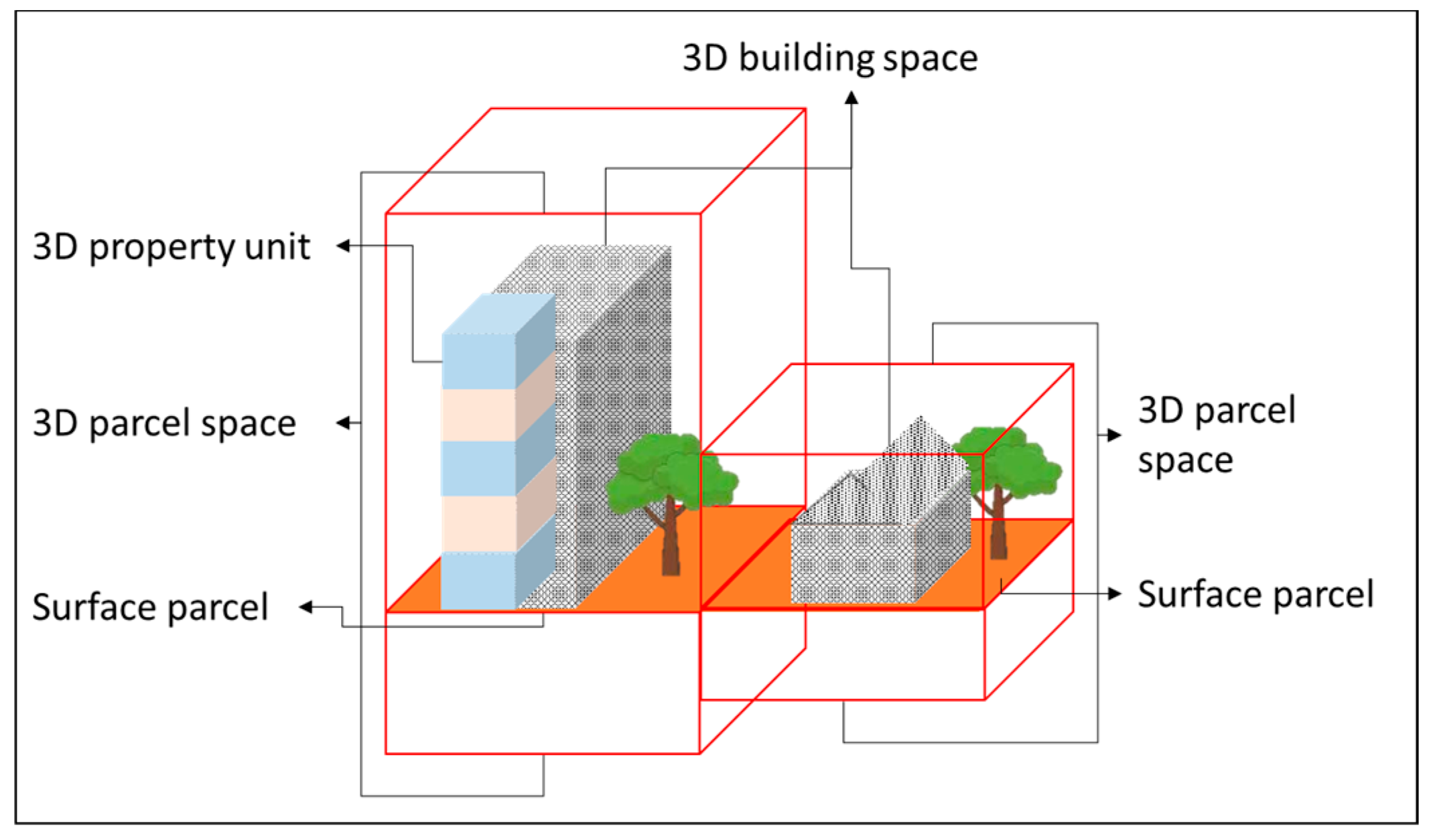
Most previous studies that modelled 3D rights and their corresponding physical buildings have primarily concentrated on strata title cases. However, the development of 3D cadastral systems is also important for other 3D-related scenarios, such as single lots or private lots. Strata title cases involve shared ownership of individual units and common property within multi-unit buildings (Figure 1—left side), whereas single or private lots refer to individually owned parcels of land and buildings without any shared ownership (Figure 1—right side). This trend has been observed in countries such as Malaysia, Israel, Greece, and Poland [5]. This is in line with regulatory developments in Indonesia, where the transition from 2D to 3D cadastral regulations has begun. However, the implementation of 3D cadastre in Indonesia is still in its early stages.
Figure 1.
Different 3D models in 3D cadastre [6].
Currently, the Government Regulation No. 1 of 2021 on Electronic Certificates introduces new mapping provisions for areas below and above the surface to regulate 3D rights. Nonetheless, legal rights are still defined based on 2D parcel boundaries. Furthermore, the regulation of vertical boundaries (3D rights) in Indonesia has been studied using 2D parcel sources [7]. In the context of fiscal cadastre, property tax is applied not only to land rights but also to buildings. For land taxation, the market price is a key factor, while building taxation is based on building assessments. Currently, building tax assessments rely on semantic records collected through field surveys for each taxable object using an analog form known as LSPOP (Lampiran Surat Pemberitahuan Objek Pajak). This process is resource-intensive and time-consuming. Additionally, property tax assessments in Indonesia still follow a mass appraisal approach, where the tax base is derived from aggregated data of surrounding tax objects within the same zone. As a result, assessments are often inaccurate. In contrast, the use of digital building models has proven effective in enabling transparent, individualized property assessments [8]. If 3D digital models representing both 3D rights and buildings are available, the implementation of tenure and fiscal functions of a 3D cadastre in Indonesia becomes feasible and significantly more efficient.
Furthermore, the Ministry of Agrarian Affairs and Spatial Planning/National Land Agency (ATR/BPN) of Indonesia has been actively modernizing its land administration systems. Through the Directorate General of Land Survey and Spatial Planning (Ditjen SPPR), initiatives such as the acceleration of land certification programs and the use of UAVs for aerial mapping have been launched. These programs, including the Complete Systematic Land Registration (PTSL), aim to improve the accuracy and efficiency of land parcel mapping by leveraging drone technology to capture high-resolution orthophotos and point clouds. Ditjen SPPR has also introduced community-driven approaches, such as participatory land parcel marking, to facilitate data verification and reduce disputes. In the meantime, the emergence of UAV-based aerial LiDAR (Light Detection and Ranging) offers further potential for the development of 3D cadastre. UAV-LiDAR can produce detailed point cloud data with high accuracy, broad spatial coverage, and relatively low cost [9]. To achieve higher levels of detail, a combination of mapping technologies, such as terrestrial mapping, is often required [10]. However, cadastral mapping implementation in Indonesia remains a sensitive issue, and UAV-based mapping is the most suitable option at present.
Although 2D parcels and some 3D building models have already been generated from UAV-photogrammetry data, point clouds produced by UAV-LiDAR offer the advantage of capturing additional features, such as exterior building walls and fences. These object classes can significantly enhance the level of detail in 3D building models. However, the utilization of point clouds representing exterior walls and fences has not yet been widely explored [11,12], where these real building boundaries are valuable for fiscal cadastre. Moreover, modelling buildings directly from point clouds, as raw 3D data sources, remains a challenging task [10,13], highlighting the need for automation. Artificial Intelligence (AI) techniques in computer vision offer a promising solution to facilitate the modelling of point clouds [12,13,14]. Nonetheless, automatic modelling still requires further development, as current methods often depend on point clouds of individual building classes or predefined 2D vector building footprints [13,15,16].
Furthermore, the positions of existing 2D parcels need to be updated. Misalignments occur due to differences in data acquisition time and technology, which indicates that the old and new data sources are different. Existing 2D parcel data in Indonesia are a collection of records gathered from the 1960s to the present day. The misalignment is caused not only by differences in mapping technologies but also by changes in the Earth’s dynamics over time. Differences in resolution and accuracy between data sources cause misalignment, where current research still relies on manual adjustments even though boundary indication is determined automatically [14,15,16]. Manual alignment is time-consuming; therefore, an automated process is necessary, where real fences as legal space boundary indicators assist in the automation process.
This research aims to develop the automation of 3D cadastral object modelling for single lots using raw UAV-LiDAR point cloud data, by utilizing point cloud features—including minimal elements that represent 3D rights and building boundaries, which is expected to enhance the geometric quality of digital 3D cadastral models. The case study of this research is in Cimahi City, Indonesia. The main objectives of this research are as follows:
- The alignment of 2D parcels, serving as the basis for 3D rights, by utilizing UAV-LiDAR point clouds of the fence class
- The modelling of more detailed 3D building models by utilizing UAV-LiDAR point clouds of the exterior wall class
2. Literature Reviews
Each country defines the priority of 3D objects in the 3D cadastre differently. Although these priorities vary, national approaches generally share a common characteristic: the prioritization of 3D rights and 3D building models as the foundational elements in 3D cadastre development [17]. Figure 1 illustrates digital models used in 3D cadastre. In many cases, 2D parcels must be aligned to generate a ‘3D parcel space’, which serves as the representation of 3D rights. This concept has been adopted by several countries, including Argentina, Malaysia, Queensland (Australia), and Croatia. In contrast, other countries define 3D rights more specifically within the frameworks of a ‘3D building space’ or ‘3D property unit’ [17]. Although Indonesia has not yet legalized the implementation of 3D rights in its cadastral system, the fundamental representation of legal rights remains the 2D parcel. Therefore, existing 2D parcels must be adjusted to align with newly available 3D data sources.
The adjustment of 2D parcels shares a similar concept with coordinate transformation, which involves converting the coordinates of a point or a set of points from one coordinate system to another [18]. Satwika et al. (2022) applied block adjustment using a least-squares procedure to correct inconsistencies in block parcels from cadastral registration maps [19]. The block adjustment method derives transformation parameters, rotation, translation, and scaling, between the vertices of the target parcels and reference vertices, which are manually marked on orthophotomaps as tie points. However, the manual marking of tie points is time-consuming, especially over large areas of interest. Alternatively, there is an algorithm for automatically aligning two point clouds by iteratively minimizing the distance between corresponding points, known as the Iterative Closest Point (ICP) algorithm [20]. ICP is widely used in computer vision, robotics, and 3D modeling due to its ability to automatically find corresponding points based on shape similarity while preserving the original geometry. Therefore, this research adopts the ICP algorithm to perform automatic adjustment of 2D parcels using UAV-LiDAR point cloud data as reference.
Moreover, several studies have addressed the challenges of automatic 3D modelling from point clouds. Yi et al. (2023) utilized point cloud data along with block partitioning and contour extraction algorithms to generate 3D volumetric building models at Level of Detail 2.2 (LOD2.2) [21]. However, the resulting roof models did not accurately represent the original roof shapes, instead producing simplified cubical forms. Additionally, incomplete data negatively affected the quality of the 3D building models. Murtiyoso et al. (2020) used building roof footprints and point cloud data to produce 3D surface models at LOD2.2. However, the presence of noise, such as vegetation surrounding the roof, significantly impacted the accuracy of the models [12]. Similarly, missing data on roof surfaces reduced the overall model quality. Peters et al. (2020) employed Digital Surface Model (DSM) data and building footprints to generate volumetric 3D digital building models at LOD1.2, LOD1.3, and LOD2.2 [11]. While their algorithm is relatively resistant to noise, it remains sensitive to incomplete data and still requires 2D building footprints as input. In contrast, Nan and Wonka (2017) proposed a method that requires only individual building point clouds. Using the Polyfit method, they constructed automatic 3D building models at LOD2.2 [22]. This method offers advantages such as robustness to both noise and incomplete data and produces 3D models that closely resemble real-world buildings. Due to these advantages, the method proposed by Nan and Wonka (2017) is adopted in this research [22].
3. Materials and Methods
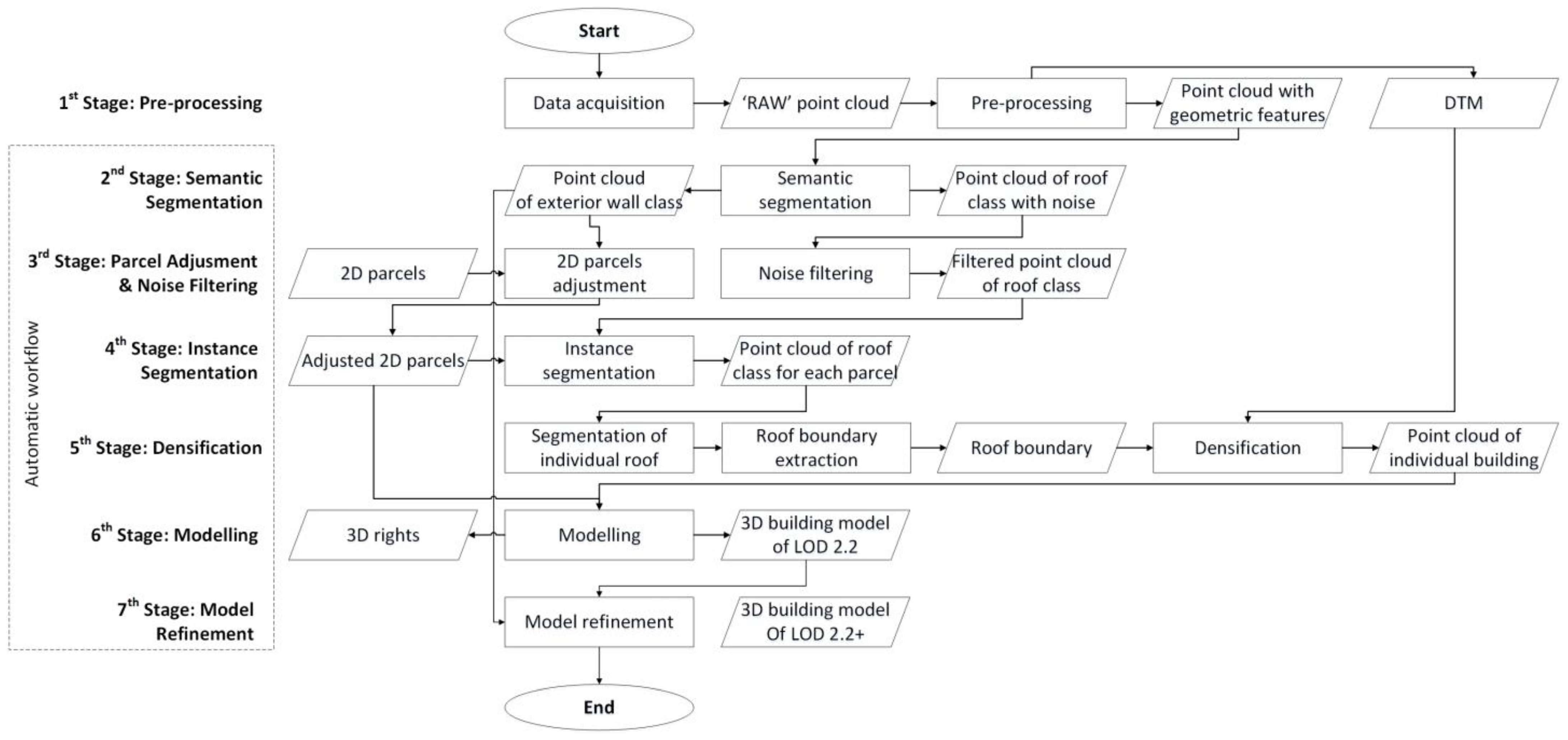
The automated framework for constructing 3D cadastral models of parcels and buildings using UAV-LiDAR consists of seven stages. This automatic workflow produces three outputs: 3D rights, a 3D building model at LOD 2.2, and a 3D building model at LOD 2.2+. The complete workflow is illustrated in Figure 2.
Figure 2.
Automatic workflow of 3D cadastral models.
3.1. Data
Primary data were derived from the acquisition by UAV-LiDAR. The acquisition technology is the gAirHawk GS-100C LiDAR system. The flight path planning is made to resemble a grid on three flight blocks. Primary data are ‘RAW’ point clouds with an accuracy of 0.025 m and 742 ppm. The density of down-sampled point clouds is 52 ppm. Secondary data consist of existing 2D parcels, which are a collection of parcels taken with various mapping technologies and at different times. The Area of Interest (AOI) is Cimahi city of Indonesia.
3.2. Preprocessing Data
‘RAW’ point clouds were processed by correcting the point cloud data using the boresight and level-arm calibration result correction parameters. After that, the strip adjustment method was applied [23]. If the color (RGB value) in the point cloud data was not satisfactory, an adjustment process was carried out using a separately processed orthophotomap. The final step in processing the ‘RAW’ point clouds was noise filtering using the Statistical Outlier Removal (SOR) technique, by assuming that the distance between a certain point and its neighbors was normally distributed, so that points falling outside the average with a 95% confidence interval were considered outliers [24].
Before the point cloud data were processed for semantic segmentation, data preprocessing was required so that the point cloud data had the features needed for the next stage. The required features were 12 in total: red, green, blue (RGB values), intensity, normal X, Y, and Z, linearity, change of curvature, planarity, anisotropy, omnivariance, and height Above the Ground Level (∆Z). Some features required an extraction process using several methods and additional data. The ∆Z feature was obtained with the help of Above the Ground Level (AGL) data, which was generated by a Digital Terrain Model (DTM) derived from point clouds of the ground class. AGL extraction was carried out automatically using several popular algorithms, namely the Cloth Simulation Filter (CSF). Each of these algorithms had its own advantages. In this research, the CSF algorithm was used because the Area of Interest (AOI) was flat, which suited the strengths of this algorithm [25]. The normal XYZ, linearity, curvature changes, planarity, anisotropy, and omnivariance features were determined by calculating the directions of maximum variance by finding the eigenvectors and eigenvalues of the covariance matrix. The RGB and intensity value features were directly obtained from the scanned point cloud data. The result of this stage was point clouds enriched with geometric features.
3.3. Semantic Segmentation
Although Deep Learning (DL) methods in AI are widely used for semantic segmentation, they typically require a large amount of training data [20,21]. Meanwhile, Indonesia has just started the transformation from 2D to 3D cadastre, which has limited 3D data sources from UAV-LiDAR. Machine Learning (ML) techniques, such as Random Forest (RF) algorithms, are incorporated to address challenges in spatial data segmentation with limited data availability [26]. The area of the AOI was small, only ±13 ha. The purpose of this stage was to obtain the roof and exterior wall classes (including façades and fences of buildings). These object classes have simple surfaces, which are suitable for the RF algorithm [27]. The RF algorithm was used in this research. The primary data were divided into areas for training, testing, and validation, each with an area percentage of 70%, 15%, and 15%, respectively. This process followed the procedure from model RF IV in Widyastuti et al. (2024) [26].
3.4. Parcels Adjustment and Noise Filtering
However, the segmentation results produced by the RF algorithm still contained noise [28]. Based on a review of filtering techniques, the projection and neighborhood-based categories were able to eliminate noise and outliers while maintaining the geometric features in point cloud data [29]. One of the popular filtering techniques is the Gaussian Mixture Model (GMM), which is included in the ML approach of unsupervised clustering techniques [30]. The GMM technique can find complex patterns and group them into cohesive and homogeneous components that represent these patterns. This technique is suitable for automatically filtering the noise resulting from segmentation by the RF algorithm.
GMM is used to filter noise. The mean and covariance values used in GMM provide better information than using only the mean, as in K-Means [30]. GMM is an unsupervised clustering technique that forms ellipsoidal clusters based on probability densities estimated using Expectation–Maximization (EM). Each cluster is modeled as a Gaussian distribution. GMM is represented as a linear combination of basic Gaussian probability distributions.
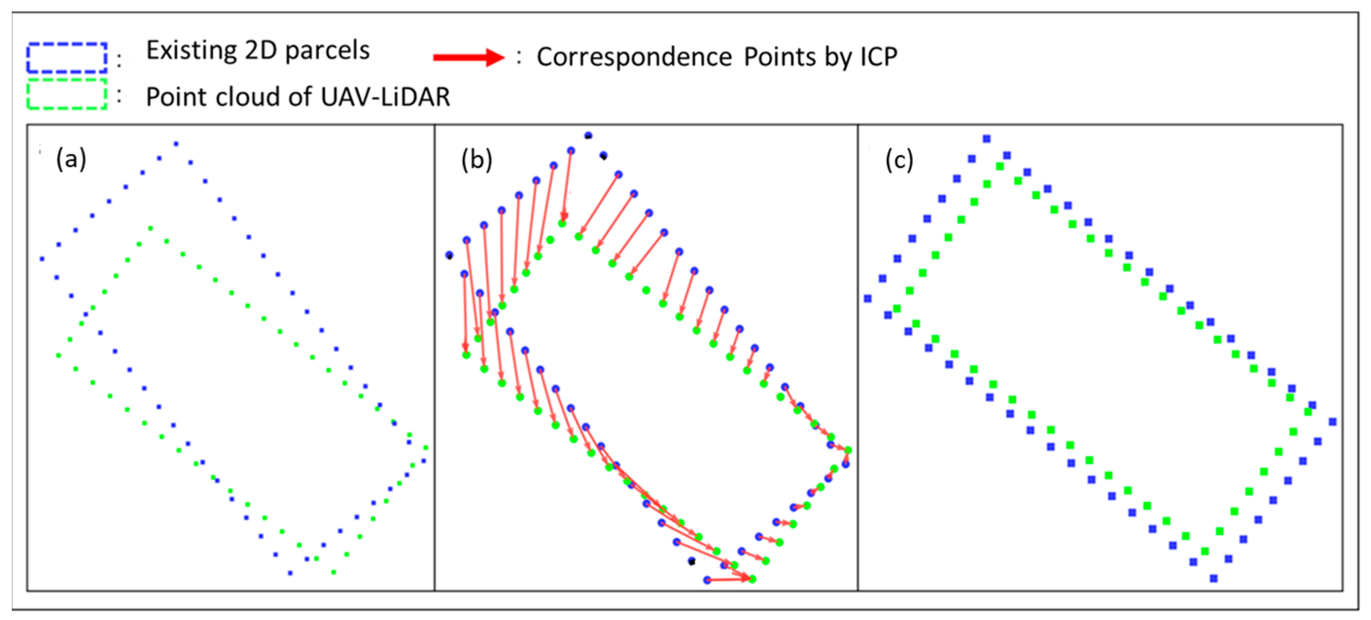
Other than the filtering process, the 2D parcels needed to be adjusted. The parcel adjustment process was an adoption of the point cloud registration method called the Iterative Closest Point (ICP) algorithm. The algorithm aims to minimize the difference between two sets of points. This algorithm was first used for point cloud registration [20]. In this algorithm, the points that are paired (correspondence points) must be identified in both sets of point clouds. Unfortunately, the geometry of the 2D parcels was in polygon vector format, which had to be converted to points before the adjustment. In addition, the radius nearest neighbor (NN) parameter was defined first. The illustration is shown in Figure 3.
Figure 3.
Illustration of parcels adjustment. (a) Data. (b) Correspondence points by ICP. (c) Adjusted 2D parcels by rigid transformation.
3.5. Instance Segmentation
The adjusted 2D parcels were used to clip the point clouds of the roof class. This step was necessary because the 3D model had to be integrated with the 2D parcels, which represent legal rights in Indonesia. The clipping process was carried out using Geographic Information System (GIS) operations.
3.6. Densification
The densification process was carried out after obtaining the roof boundary. To obtain the roof boundary, segmentation of individual roofs was needed. There were three steps in this stage, as follows:
- Segmentation of the individual roofWhile Murtiyoso (2020) used the region growing algorithm to perform part segmentation of roof point clouds [12], this research used the region growing algorithm to segment individual roofs. The optimal threshold value for change of curvature is typically obtained using the average value and deviation at a certain confidence interval across the entire point cloud data to be segmented [31]. However, in this research, the threshold value for change of curvature was set differently. For the purpose of segmentation, the threshold was determined in advance as 30°, without using the average value and deviation at a certain confidence interval. The value of the change of curvature threshold was determined by the common angles in roof construction in Indonesia [32]. Furthermore, the other threshold—the minimum number of points in one region was decided based on the area of common roof construction in Indonesia, which is 4 m2.
- Roof boundary extractionThe Hull algorithm is the most efficient and closest method that is designed to connect vertices in the reconstruction of geometric shapes [33]. The Concave-Hull algorithm was applied in this research to develop the roof boundary. The Concave-Hull connects the point set with a concave space, allowing the formation of angles between points [33]. The Concave-Hull technique is defined such that the shape containing all points does not have any angle exceeding 180°.
- DensificationThe extracted roof boundary was used to generate the point clouds of the exterior walls. In addition, the heights of the ground and roof were needed. The ground height was based on the DTM, while the maximum roof height was obtained from the maximum height of the segmented point clouds of the roof class to avoid gaps between roofs. The generation of façade point clouds was carried out using GIS operations. Moreover, the ground itself was generated using the bounding boxes of the point clouds of the roof class. The point clouds of individual buildings, consisting of roof, façade, and ground, were the final product of this step.
3.7. 3D Cadastral Modelling
This stage discusses four concepts of 3D cadastral modelling: the modelling concept, the modelling process of the 3D cadastral model, model refinement, and 3D building model validation.
3.7.1. Concept of 3D Cadastral Model
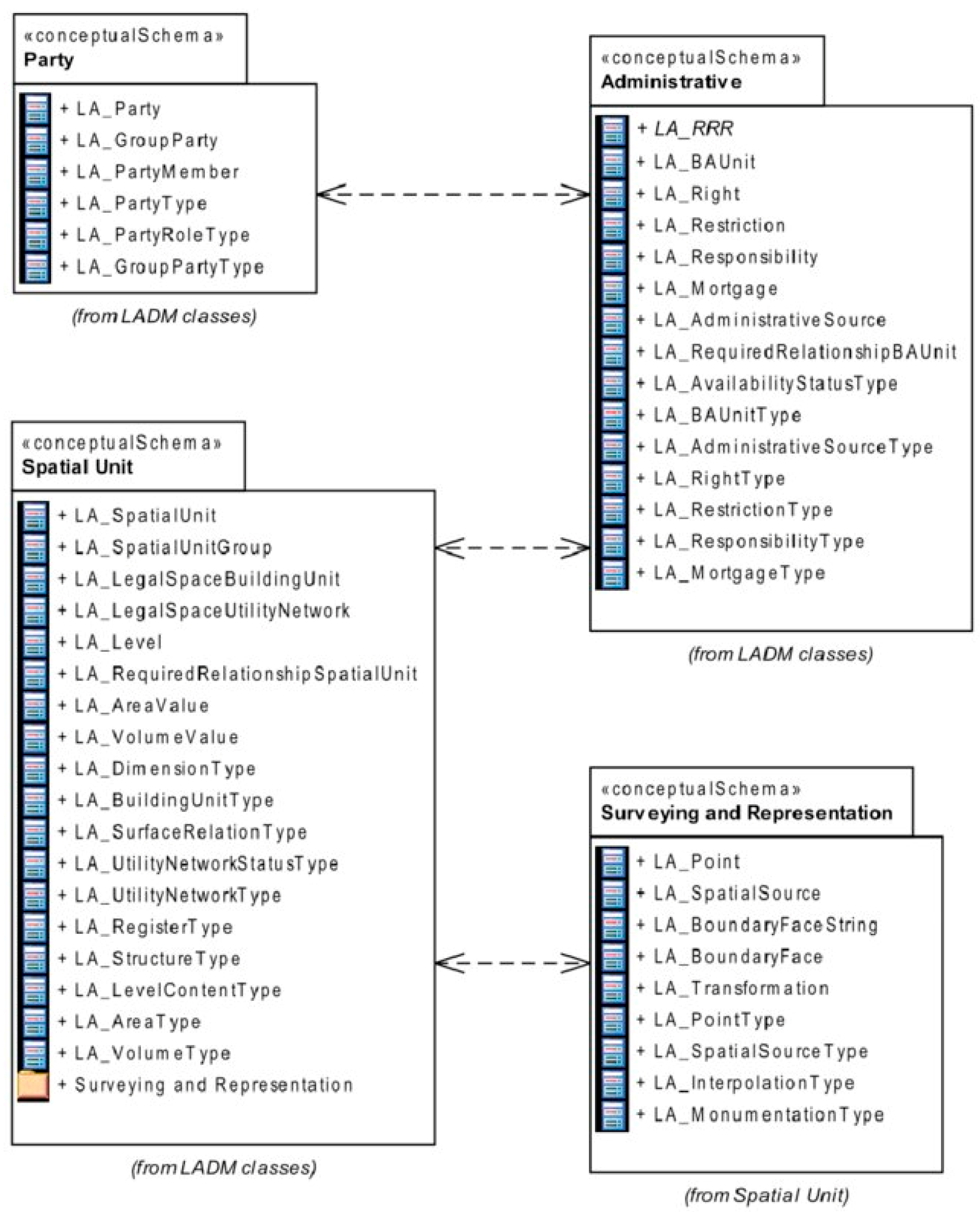
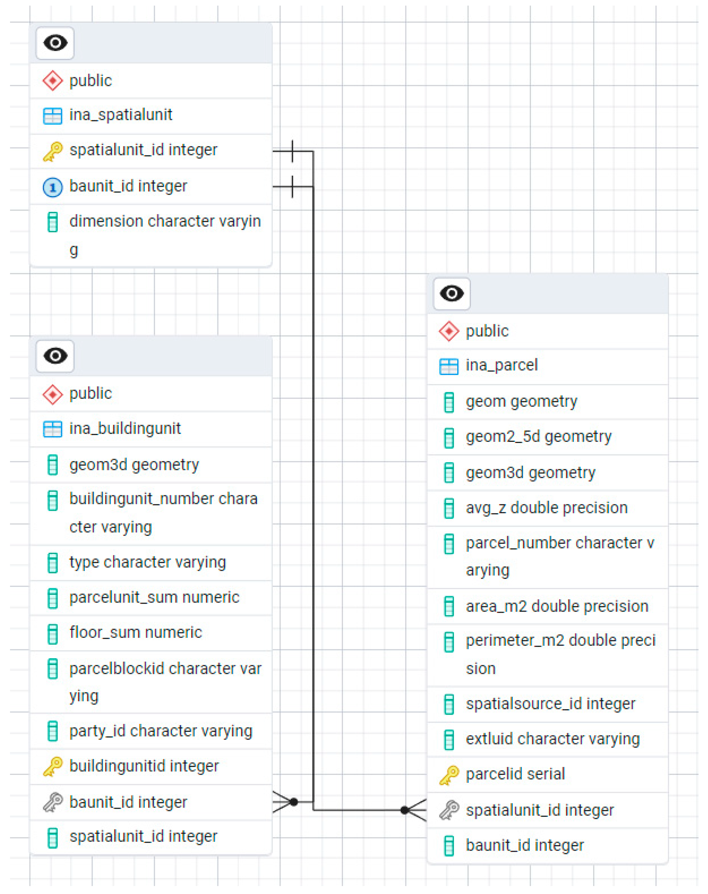
The thesis by Sitarani Safitri (2014) described how to develop a conceptual architecture of cadastral data management (CDM) by implementing 3D cadastre and the Land Administration Domain Model (LADM) [34]. The conceptual architecture was designed based on CDM requirements and LADM, with the Country Profile of Indonesia. The CDM requirements were identified from the perspective of Spatial Data Infrastructure (SDI) components. The data consisted of 3D building models, spatial data of 2D geometries of parcels, and some non-spatial data. The implementation of 3D cadastre in Indonesia adopted the hybrid cadastre model from Stoter (2004). The concept of a hybrid cadastre is to preserve the current 2D registration and add a 3D component to the registration system. The ‘ina_parcel’ is represented as a 2D geometry, which is inherited from the current 2D registration system. Meanwhile, ‘ina_buildingunit’ is represented as a 3D building unit in strata title or 3D building geometry in a single lot. The adaptation of LADM into the 3D cadastre for Indonesia shows the correlation of ‘ina_parcel’ (2D) and ‘ina_buildingunit’ (3D) (Figure 4). In Figure 4, the numbers beside the association lines represent multiplicity based on UML (Unified Modeling Language) notation, which defines how many instances of a class can be associated with another. The cardinalities indicate the number of possible instances in a relationship, where ‘1’ means exactly one (a required instance), ‘0..1’ means zero or one (optional), ‘0..*’ means zero or many (no upper limit), and ‘1..*’ means one or many (at least one instance is required). These cardinalities indicate the relationships between feature types in the model. For example, one ‘ina_parcel’ can be related to multiple ‘ina_buildingunit’ objects (0..*), while each ‘ina_buildingunit’ must be associated with exactly one ‘ina_parcel’. This structure reflects the real-world relationship between land parcels and the buildings constructed on them. The model is implemented in PostgreSQL.
Figure 4.
Adaptation of LADM into 3D Cadastre for Indonesia of ina_spatial ina_buildingunit (3D) [34]. Notations 0..*, 0..1, 1..*, and 1 represent cardinality or multiplicity.
The diagram in Figure 4 illustrates the development of LADM based on ISO 19152:2012 [35] (Figure 5), adapted to the Indonesian context. However, the LADM concept presented in Figure 4 is primarily intended for tenure cadastre, which represents the boundaries of 3D rights and 3D physical buildings. Nevertheless, since this research focuses more on the automation of geometric modeling of 3D cadastral objects, the adoption of the LADM concept in Figure 4 is considered sufficiently representative for this study.
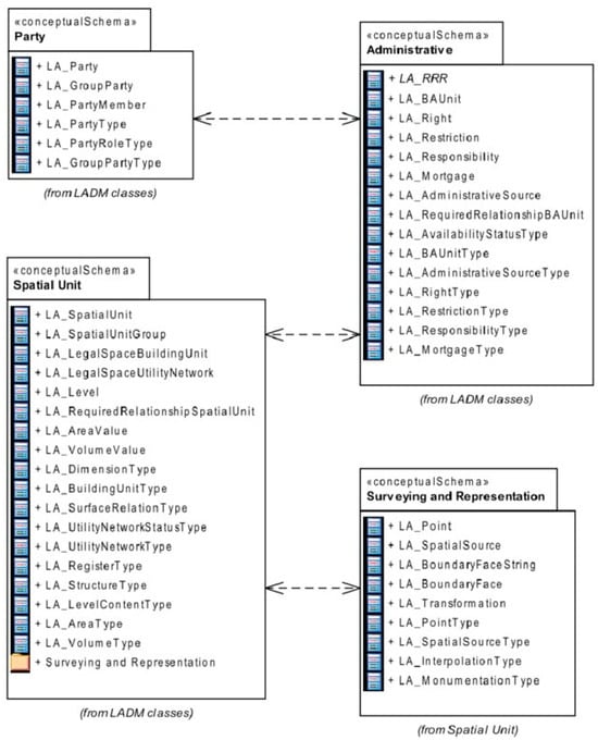
Figure 5.
LADM packages and sub-packages with their respective classes (Geographic Information-Land Administration Domain Model (LADM), 2012).
The representation of the 3D cadastral model structure is a polyhedron. The advantages of polyhedron data structures for cadastral purposes stand out the most due to their easy implementation [36] and their ability to be spatially modeled because of their homogeneous space with respect to ownership [37]. Therefore, this research used a polyhedron data structure in the 3D model.
3.7.2. Modelling Process of 3D Cadastral Model
After obtaining all point clouds of individual buildings, the point clouds were then modelled using the PolyFit algorithm [22]. This algorithm is chosen because it has the advantage of handling rough edges in point clouds, which are commonly found along object boundaries. It is also capable of generating complex models of real-world buildings. Although the point clouds for individual buildings had to be generated beforehand, they had already been produced in the previous stages. The PolyFit algorithm consists of four main steps: (1) plane extraction; (2) plane refinement; (3) pairwise intersection; and (4) optimization. The PolyFit algorithm is illustrated in Figure 6. The plane extraction process was performed using Easy3D-v2.5.3 by Nan & Wonka (2017) (see Supplementary Materials). The parameters used in the algorithm were the number of points to calculate the normal and the minimum number of points to generate planes, which were 100 points and 200 points, respectively. These parameters were based on considerations of the real size of building components. Other than that, the default parameters were used [22]. For the subsequent processes plane refinement, pairwise intersection, and optimization, the Polygonal Surface Reconstruction-Polyfit_v1.5 tool by Nan & Wonka (2017) was used (see Supplementary Materials). This stage produced the 3D building model in LOD 2.2. LoD2.2 refers to a refinement of the standard LoD2 building model, offering improved geometric detail on elements such as facades and roof structures. These enhancements, often derived from LiDAR or photogrammetric data, make the model more accurate without reaching the complexity or cost of full LoD3 representations [10]. As such, LoD2.2 serves as an intermediate level between LoD2 and LoD3, balancing realism with efficiency.
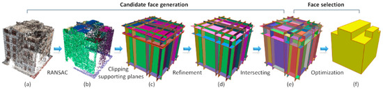
Figure 6.
Illustration of the Polyfit algorithm in 3D modelling. (a) Input point cloud. (b) Planar segments. (c) Supporting planes of the initial planar segments. (d) Supporting planes of the refined planar segments. (e) Candidate faces. (f) Reconstructed model [22].
3.7.3. Model Refinement
The previous step was obtaining the 3D building model in a polyhedron data structure consisting of many faces with a varying number of vertices (Figure 7). However, the 3D model with a polyhedron data structure cannot identify which parts are the roof, façade, or ground floor. The base 3D model itself is modelled from point clouds of the roof class, which can be recognized as the minimum height limit of the ceiling. Therefore, to optimize the utilization of the exterior wall/fence class, the previous 3D building model was cut into two parts based on the height information from the roof point clouds, namely, the ‘roof of the building’ and the ‘body of the building’. The ‘body of the building’ part was then updated. The updated 3D ‘body of the building’ is illustrated in Figure 7.
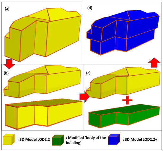
Figure 7.
The 3D building model update process. (a) Previous 3D building model. (b) 3D building model was divided into two parts. (c) Modified ‘body of the building’ and original ‘roof of the building’. (d) A unified model of the roof and body of the building.
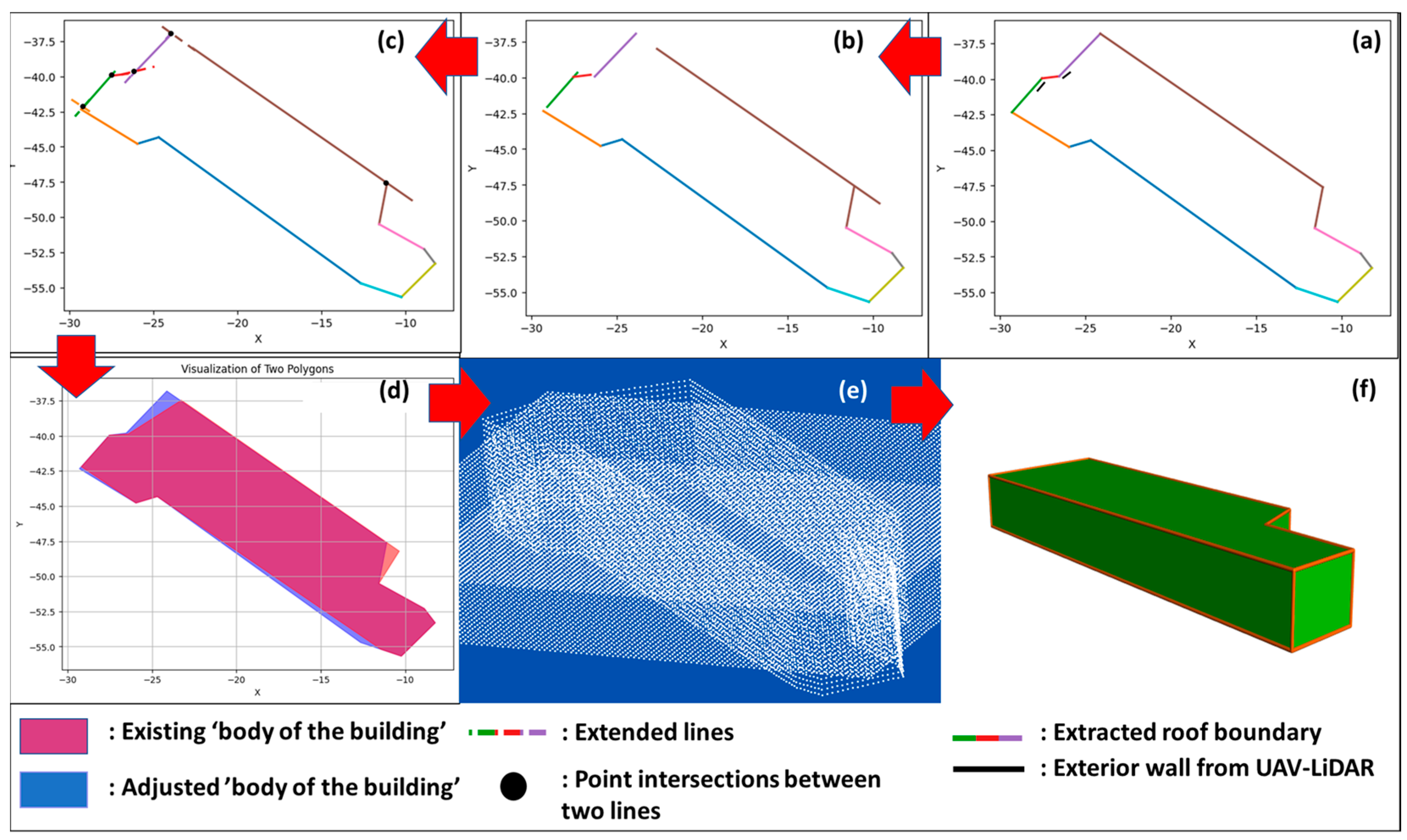
The ‘body of the building’ was updated using simple orthogonality (illustrated in Figure 8). Figure 8a shows the extracted roof boundary (colorful line) and the existing line of the exterior walls from UAV-LiDAR. The process of updating the ‘body of the building’ was as follows:

Figure 8.
Process of updating the 3D ‘body of the building’ model. (a) Extracted roof boundary. (b) Translation of parallel lines. (c) Extended line segments. (d) Original and updated boundary of the ‘body of the building’. (e) Individual point clouds of the ‘body of the building’. (f) Updated 3D model of ‘body of the building’.
- The first rule was set by using the nearest radius search of the existing line for each segment in the extracted roof boundary.
- If the existing line was found, the parallelism between the two lines was checked. If the two lines were parallel, the position of the roof boundary line segment was shifted. This process produced gaps between roof boundary line segments or intersections (Figure 8b).
- The next step was defined by three rules. (i) If a gap existed, an extended line was used to find intersections between two adjacent segments; (ii) if intersections existed, the parallelism between the two segments was checked. If the segments were parallel, they were merged into one line; if not, the intersections between the segments were identified; (iii) If the middle nodes were in the same location, no changes were made between segments. This was illustrated in Figure 8c.
- The result from step c was the updated boundary of the ‘body of the building’. The point clouds of the ‘body of the building’ were then generated based on this boundary (Figure 8e).
- The final step in updating the ‘body of the building’ was carried out using the PolyFit method. The result of the updated ‘body of the building’ is shown in Figure 8f.
3.7.4. 3D Building Models Validation
The validation process was conducted by comparing the area of the extracted 3D building models with the referenced 3D building models. The referenced 3D building models were obtained through a manual process. The 3D reference data combined data from UAV-LiDAR with additional data acquired using a Simultaneous Localization and Mapping (SLAM) scanner, with the aim of obtaining a more complete view of the exterior walls of the building; it can scan large areas quickly. The SLAM scanner uses the GS-100 Geosun LiDAR product, which, based on its specifications, offers more precise absolute accuracy compared to that of UAV-LiDAR.
4. Results
4.1. Primary Data
Primary data were obtained from acquisition by the LiDAR system, which produced point cloud data with an accuracy of Horizontal Root Mean Square Error (RMSEH) = 0.031 m and Vertical Root Mean Square Error (RMSEV) = 0.030 m. The RMSEH and RMSEV values were lower than the LiDAR specification accuracy of <0.056 m. In addition, the RMSEH and RMSEV values met the criteria for producing digital maps with first-class quality at a 1:200 scale, based on the National Standard for Spatial Data Accuracy (US Federal Geographic Data Committee). In relation to 3D modeling needs, RMSEH and RMSEV are within the global accuracy range for LOD 3 models (Open Geospatial Consortium, OGC).
4.2. Semantic Segmentation Results
The result of this stage refers to the findings of Widyastuti et al. (2024) in RF Model IV [26]. There were five object classes: ground, vegetation, cars, roofs, and exterior walls. The Overall Accuracy (OA) score was 94.85%, with F1 scores for the classes as follows: ground—92.95%, vegetation—89.06%, cars—0%, roof—97.3%, and exterior walls—91.86%. The important object classes for this research are buildings and exterior walls, which gave satisfactory results.
4.3. Parcel Adjustment and Noise Filtering Results
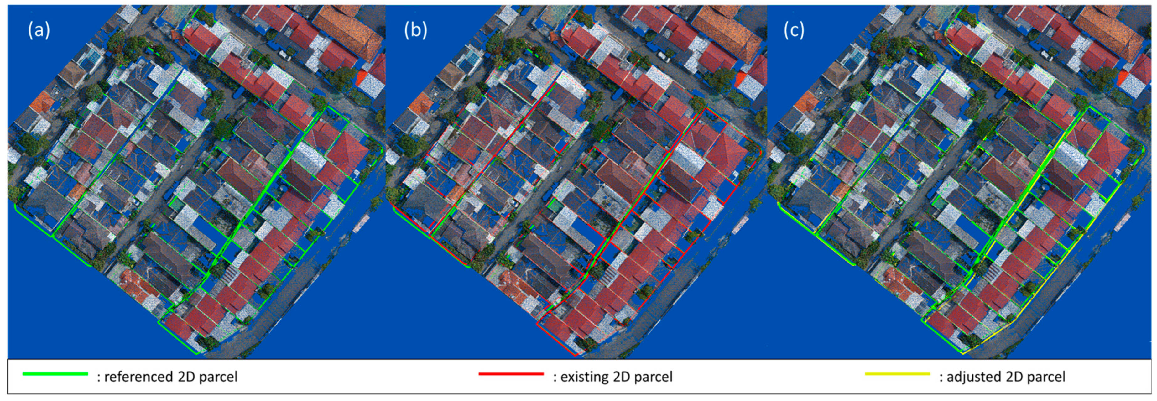
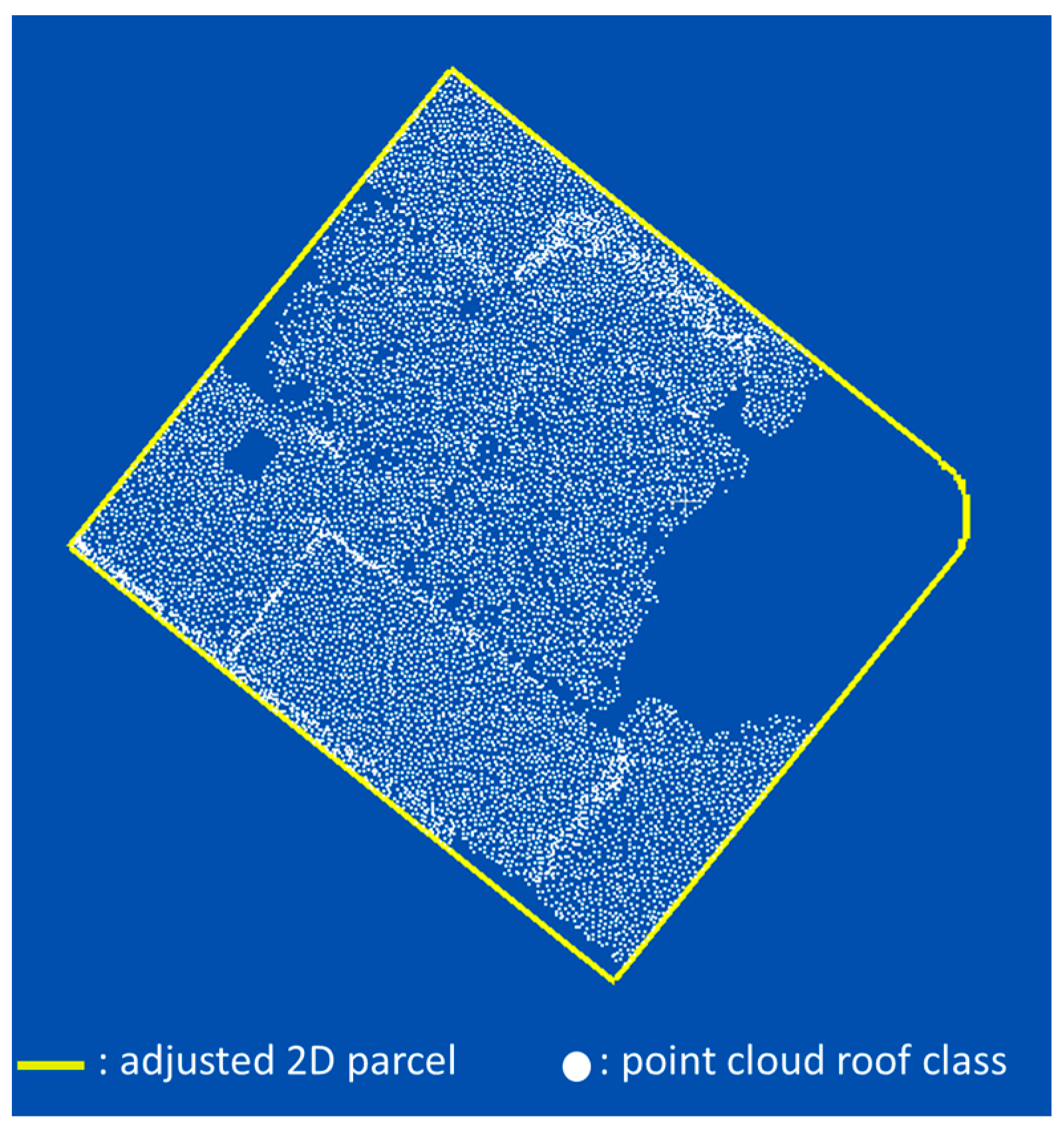
This stage produced the adjusted 2D parcels. The existing 2D parcels and adjusted 2D parcels were illustrated in Figure 9. The adjustment using the ICP algorithm corrected the positions to be closer to the actual locations. The green lines showed the referenced 2D parcels created by manual digitization, so that the position of the 2D parcels matched the position of the point cloud data (Figure 9a). Meanwhile, the red lines showed the existing 2D parcels before adjustment (Figure 9b). The yellow lines showed the adjusted 2D parcels (Figure 9c). The RMSEH of the existing 2D parcels relative to the referenced 2D parcels was 1.19 m, while the RMSEH of the adjusted 2D parcels was 0.612 m. There was a decrease in RMSEH. An RMSEH of 0.612 does not meet the absolute accuracy requirement for modelling LOD3 buildings according to OGC standards, but it does fall within the absolute accuracy threshold for LOD2 buildings, as 0.612 m < 2 m.
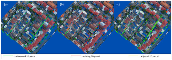
Figure 9.
Overlay of point clouds of roof class. (a) Referenced 2D parcels. (b) Referenced and existing 2D parcels. (c) Referenced and adjusted 2D parcels.
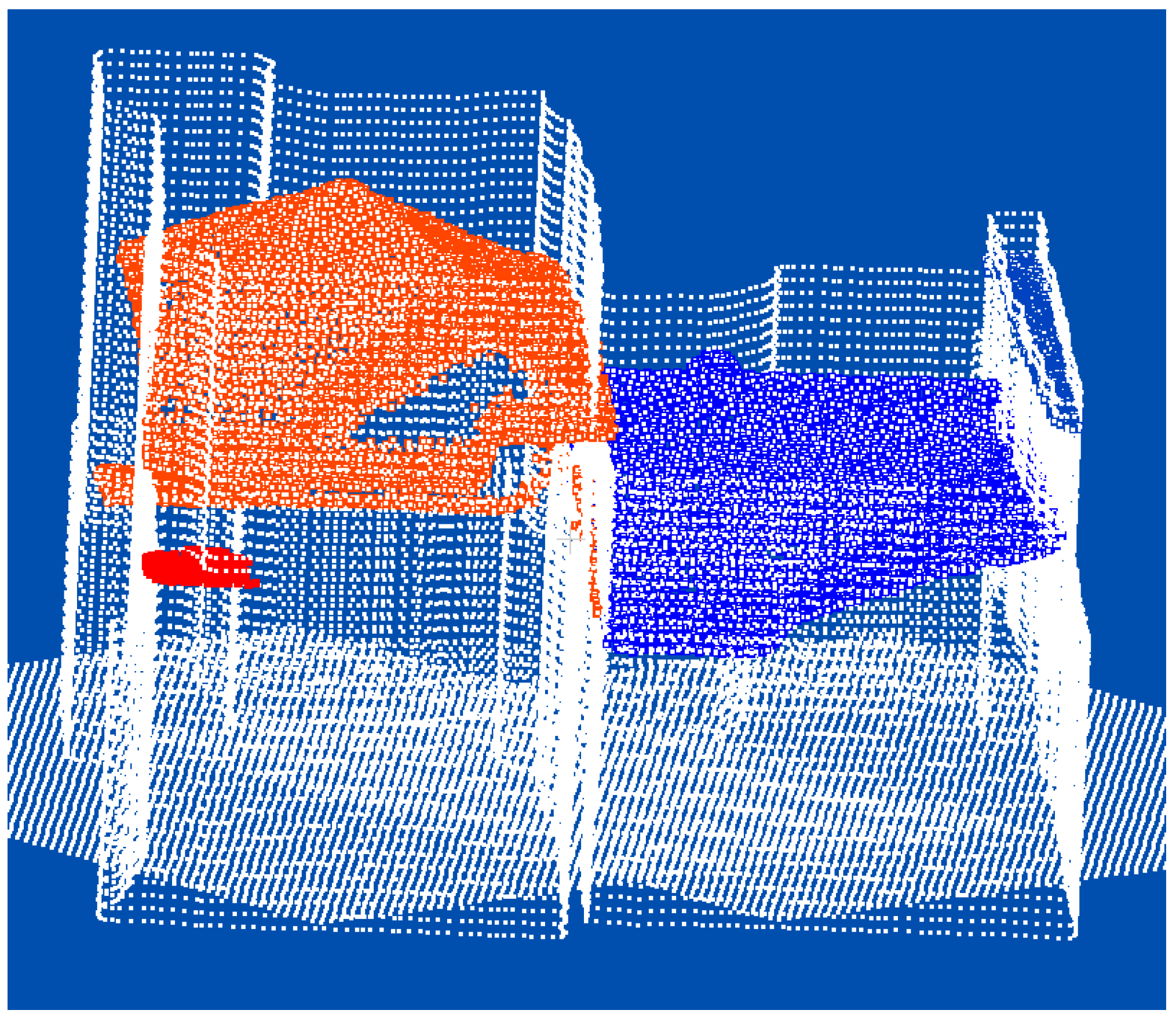
Previously, in the segmentation phase, several point clouds were classified as roof class, but some of them actually belonged to the vegetation class. This misclassification occurred in areas with dense vegetation. Fortunately, the GMM technique was able to identify them as noise, as shown in Figure 10. The light blue points in Figure 10 show the result of noise filtering, most of which should have been classified as vegetation. Nonetheless, several point clouds from the roof class were also identified as noise. The GMM technique not only identified noise that should belong to other object classes but also filtered points within the roof class. The GMM technique successfully removes 86% of the noise.
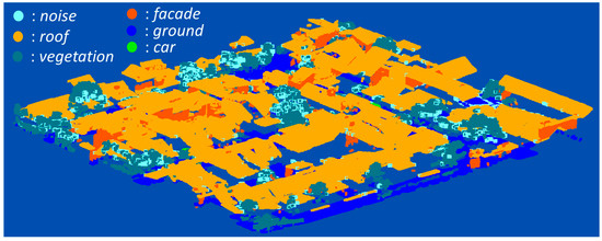
Figure 10.
Noise (light blue points) distribution of the segmented point clouds in the roof class.
4.4. Instance Segmentation Results
This stage produced the roofs of each parcel by clipping the filtered point clouds of the roof class with the adjusted 2D parcels. Figure 11 illustrates the resulting point clouds.

Figure 11.
Filtered point clouds of the roof class of each parcel.
4.5. Densification Results
Previously, the point clouds in each parcel were provided (Figure 11). Furthermore, the individual roof segmentation using the region growing algorithm produced point clouds of individual roofs in each parcel (Figure 12a). After the individual roof point clouds (segmented point clouds) were obtained, the next step was to generate the boundary of each roof in each parcel (Figure 12b). This roof boundary was used to generate the façade of the buildings. In addition, the DTM, which was generated from point clouds, was used to complete the ground point clouds of each individual building (Figure 13). This process was called point cloud densification.
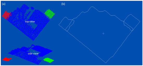
Figure 12.
(a) Individual point clouds of the roof in a parcel; (b) 2D vector of each roof boundary.
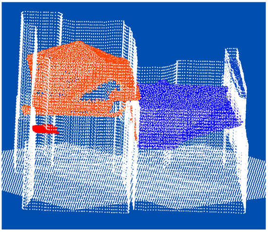
Figure 13.
Complete point clouds of two individual buildings.
4.6. 3D Modelling
After the point clouds of individual buildings were obtained, the next step was to build a 3D digital model of each building using the PolyFit method. In addition, a 3D rights space was extruded from the 2D vector data of the land parcel boundaries. The visualization is shown in Figure 14. Out of a total of 45 buildings that were modeled, two buildings had irregular shapes. This occurred because the source data for the roof class point clouds was incomplete—less than 50% of the expected data was captured. The 3D building model was represented in a polyhedron data structure, where the solid model consisted of many surfaces (Figure 15).

Figure 14.
The 3D models of 3D Rights and Building of LOD 2.2.
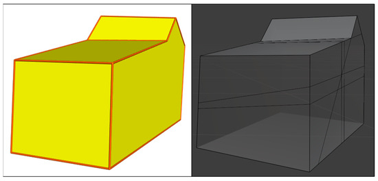
Figure 15.
Polyhedron structure of a 3D building model.
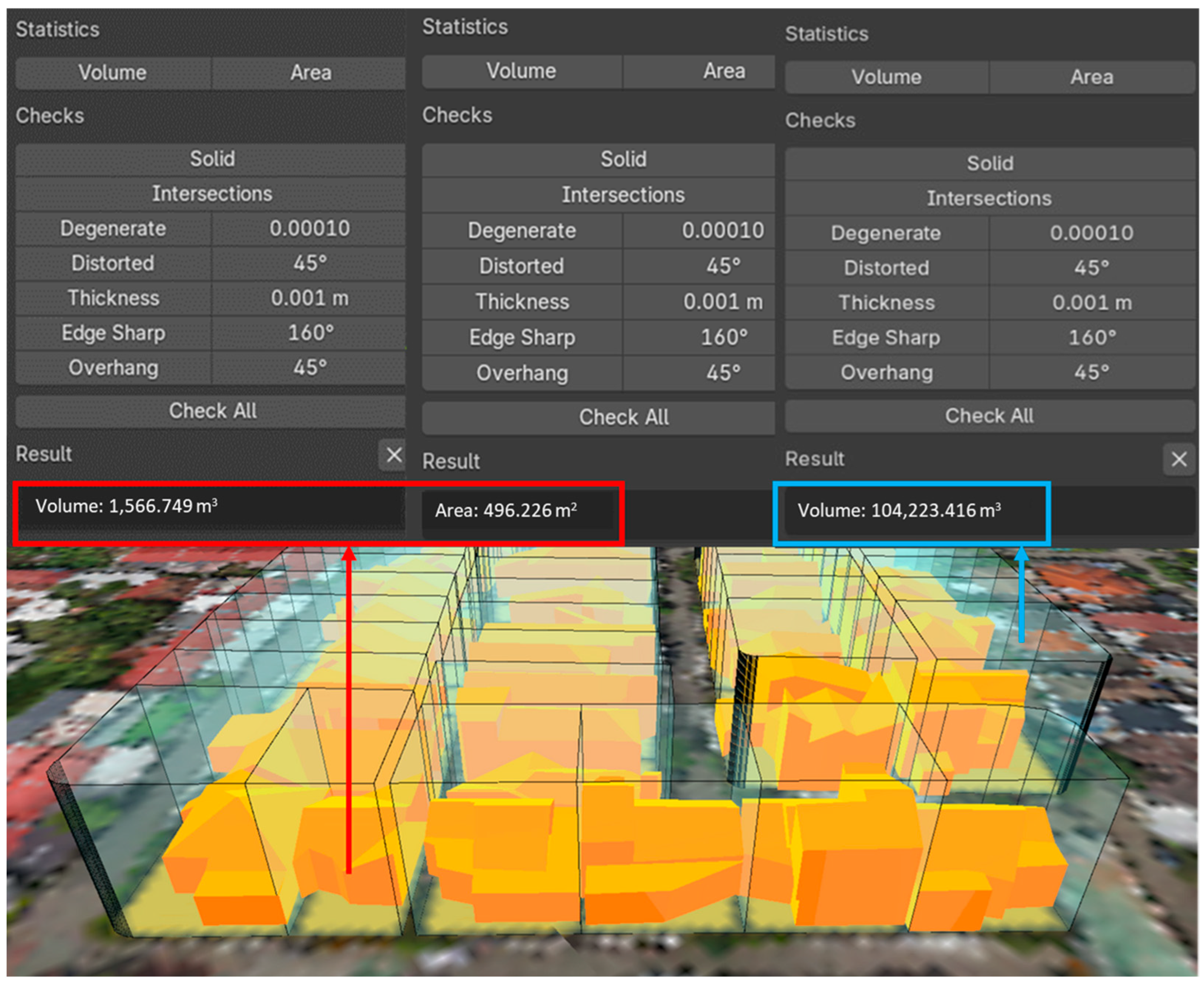
Based on the GML standard for building models, the digital building models were classified as Level of Detail (LOD) 2.2 [10]. Additional geometric semantics that were obtained from the models included building surface area, building volume, and the volume of the 3D right. The 3D cadastral models are illustrated in Figure 14. The red lines and rectangles show the geometric dimensions of the 3D building models, while the blue lines and rectangles represent the geometric dimensions of the 3D rights model.
Furthermore, other semantic information was generated through automated processes—for example, the floor area, which was derived from the extracted roof boundary. An estimate of the number of floor levels was also provided based on the height of the segmented individual roof (Table 1). The identification of roof height enables the floor area to be distinguished by level—such as floor 1 area, floor 2 area, floor 3 area, and so on—as shown in Table 1.

Table 1.
Semantic information of the 3D building model of LOD 2.2 by the products of some automatic process.
4.7. 3D Building Model Refinement
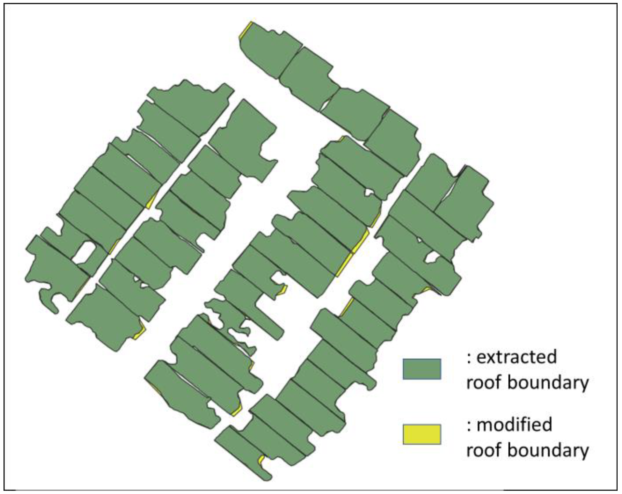
The 3D building model refinement utilized exterior walls from the segmented point clouds. The point clouds of exterior walls were transformed into 2D lines using GIS (Geographic Information System) operations. These 2D lines of exterior walls were used as reference lines. On the other hand, the 3D building model was projected into horizontal space to define the building boundary. This building boundary consisted of line segments. These line segments were shifted to align with the actual exterior wall positions (reference lines). The modified 2D building boundary and the reference lines of the exterior walls are shown in Figure 16. Although the updated floor boundary was not significantly visible in Figure 16, the RMSEH of the first floor area before and after the boundary update was approximately ±3.8 m2.

Figure 16.
Overlay of extracted roof boundary and modified roof boundary.
Another refinement was that the 3D building model was divided into two parts, the ‘body of the building’ and the ‘roof of the building’. As a result, the volume was divided into these two components of the 3D model (Figure 16). The geometric semantics of the 3D model in LOD 2.2+ were distinguished by the volume and area of the ‘roof of building’ (represented by red rectangles in Figure 17), the volume and area of the ‘body of the building’ (green rectangles in Figure 17), and the volume of the 3D rights (blue rectangles in Figure 17). The semantic information of the updated 3D building model has the same information as the previously 3D building model, as in Table 1.
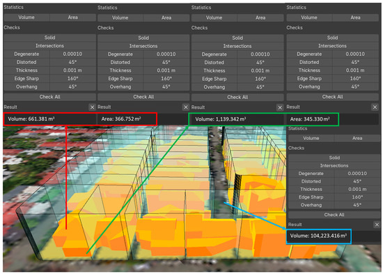
Figure 17.
The 3D models of 3D Rights and Building of LOD 2.2+.
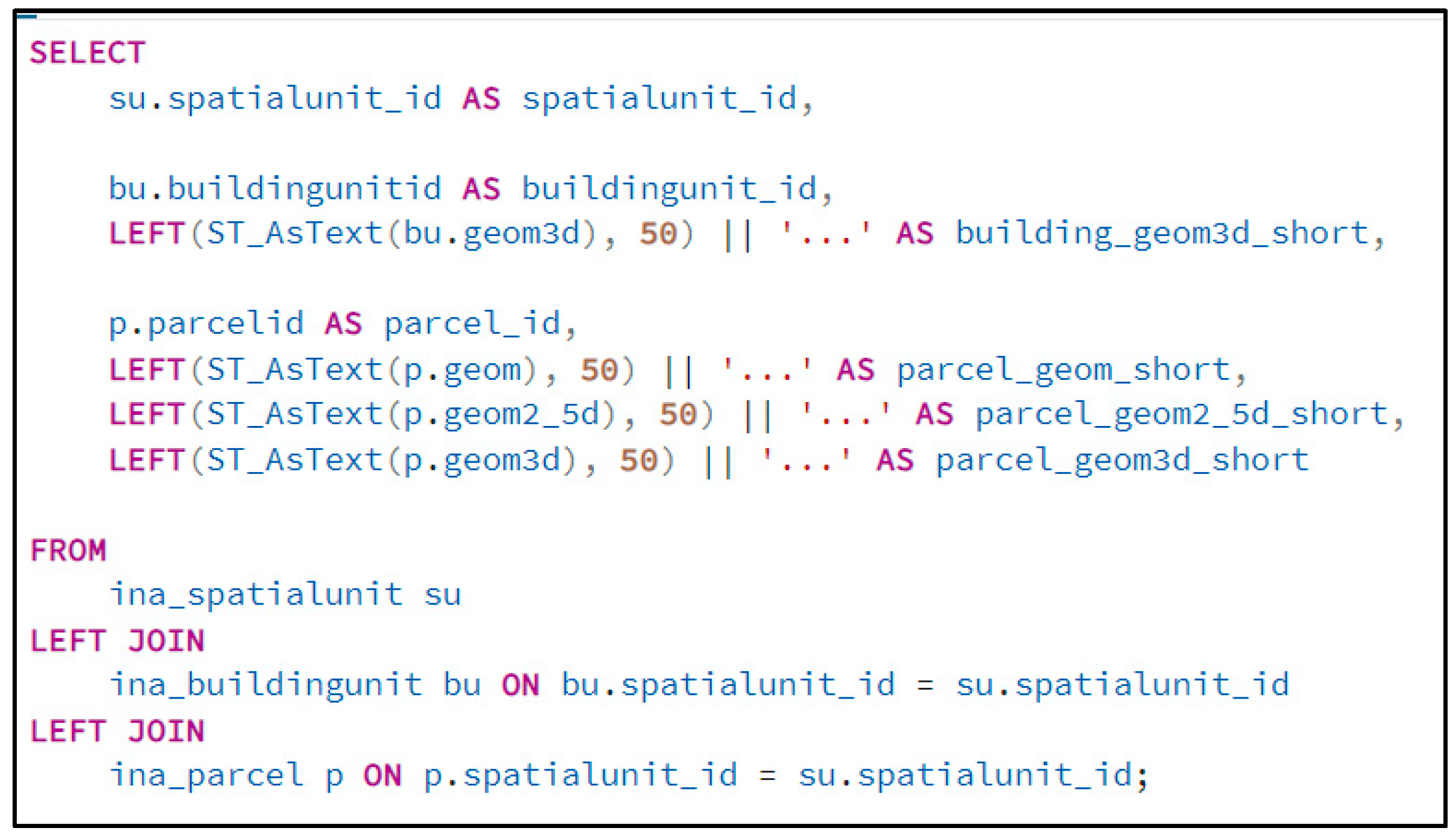
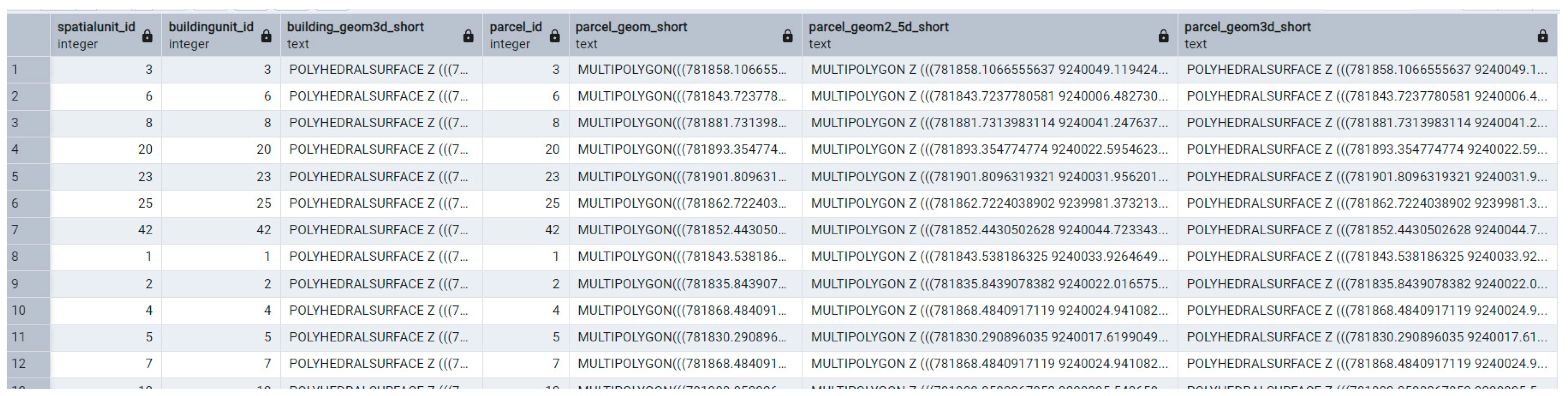
After the 3D cadastral model was obtained, the next stage was the implementation of the 3D model into the database, adopting the conceptual model of Indonesia’s LADM by Sitarani (2014). The implementation is shown in Figure 18. The entity ‘ina_parcel’ contained the digital model of 3D rights with 2D, 2.5D, and 3D geometries. The 2.5D geometries were needed to add height values from the DTM to each of their vertices. Then, the 3D geometries of the 3D parcels were generated based on the 2.5D geometries. In addition, ‘ina_buildingunit’ contained the 3D building model in a polyhedral data structure. Both entities were connected to ‘ina_spatialunit’, where the RRR (Rights, Restrictions, and Responsibilities) was linked. A query (Figure 19) was used to verify whether the model implementation was functioning correctly. Figure 20 shows the result of the query which connect each classes such as ‘ina_spatialunit’ (spatialunit_id), ‘ina_buildingunit’ (buildingunit_id, building_geom3d_short), ‘ina_parcel’ (parcel_id, parcel_geom2_5d_short, parcel_geom3d_short). The geometry columns in the table contain coordinate values representing the vertices of each shape. For example, the ‘POLYHEDRALSURFACE Z’ format stores 3D surfaces as a collection of connected planar polygons defined by their vertex coordinates.. The realization of the spatial unit of the 3D cadastre was visualized in QGIS software version 3.34, which was used to connect to the database (Figure 21).
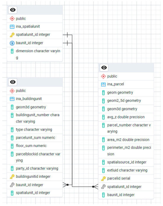
Figure 18.
Implemented conceptual model of ‘ina_spatialunit’ of Indonesia’s LADM.
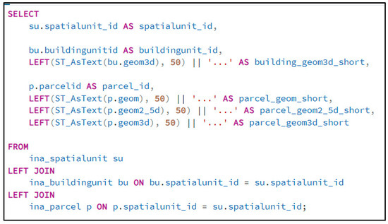
Figure 19.
Query syntax to check the relationship of ‘ina_spatialunit’, ‘ina_parcel’, and ‘ina_buildingunit’ is working.
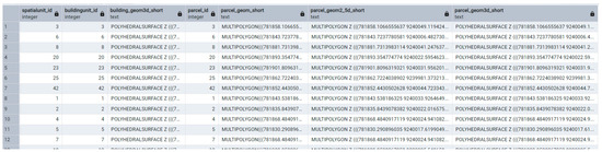
Figure 20.
Result of the query checking.
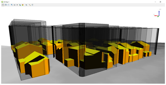
Figure 21.
Visualization of 3D Right and building model in QGIS software.
5. Discussion
The automated framework successfully generated 3D rights and building models using UAV-LiDAR point clouds through a sequential process: semantic segmentation, noise filtering, parcel adjustment, 3D rights generation, point cloud densification, 3D modelling, and refinement. The important classes of segmented point clouds for this research are ground, roof, and exterior wall. The point clouds of the roof class still contain noise, which needs to be eliminated first through a process called noise filtering.
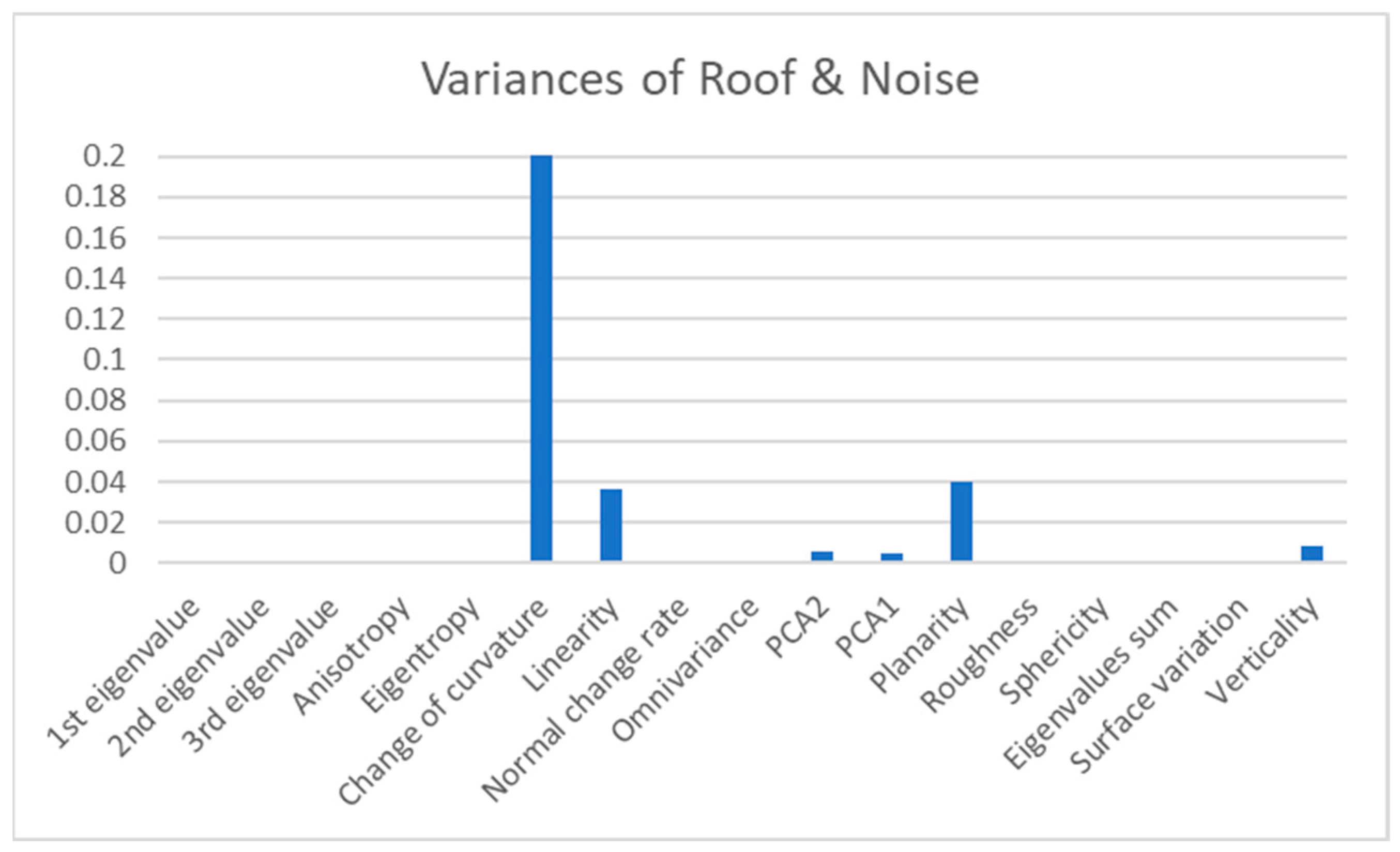
As mentioned previously, the GMM technique is an unsupervised method that separates noise within the roof class using significant geometric features. The features that enhance the performance of the GMM technique are change of curvature, linearity, planarity, and verticality (Figure 22). These four features exhibit high variance in the segmented point clouds of the roof class. High variance indicates that these features can help distinguish between actual roof points and noise. Noise filtering not only distinguishes between roof and non-roof classes but also identifies noise within the roof class itself. The success rate of noise filtering using these features was 86%, although it also eliminated 4% of valid roof-class points.
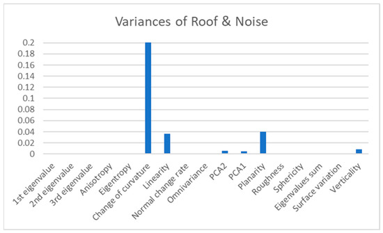
Figure 22.
Variances of geometric features of the roof class with noise.
The next stage was parcel adjustment. The adjustment process produced satisfactory results. The RMSEH was reduced from 1.19 m to 0.612 m. However, despite this reduction, the range of residual errors remains quite large (0.008–1.626 m). This suggests that the spatial alignment of each parcel relative to the LiDAR point clouds varies significantly. This variation likely results from inconsistencies in the existing 2D parcel data, which were collected using different tools and during different acquisition periods. Nevertheless, the ICP algorithm is able to generate correspondence points between the existing parcels and the reference data based on geometric similarity. This method can be further developed to address misalignments caused by these temporal and technological discrepancies.
The adjusted 2D parcels were used to clip the point clouds of the roof class. This step was necessary to fulfill the requirements of the spatial unit entity in Indonesia’s LADM [6,38]. In Indonesia, ownership and rights are based on 2D parcels, which can be extended into 3D rights. The 2D parcel is the fundamental spatial unit for land tenure and land valuation in Indonesia [39].
Furthermore, to generate a 3D building model using the PolyFit method, the point clouds needed to be complete for each individual building, including the roof, exterior wall of the building, and ground floor. To achieve this, the roof had to be segmented as an individual roof, rather than as parts of a roof. With the advantages of the region growing algorithm, the grouping result depends on specific threshold values [40]. This is consistent with Kang et al. (2020), who stated that the region growing algorithm can be used to segment point cloud data, where the type of segmentation is not specifically stated, but the specified threshold value affects the segmentation results [31]. The optimal threshold value for the change of curvature is generally obtained by using the average and deviation at a certain confidence interval across the entire point cloud dataset. However, in this study, the threshold value for the change of curvature was set slightly differently. To obtain individual roofs, the change of curvature threshold was determined in advance without relying on the average and deviation. The threshold value was based on the roof curvature standard in Indonesia, which is 30° [32]. Additionally, the nearest neighbor radius used to calculate geometric features was set at 1 m, referring to the minimum roof length characteristic in Indonesia. These thresholds failed to segment the individual roof of one parcel out of 45. This failure was caused by incomplete roof point cloud data, which created holes between points on the roof and led to anomalies in the change of curvature located in the middle part of the roof (Figure 23).
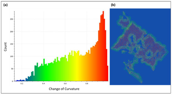
Figure 23.
Variances of geometric features of a failed segmented individual roof. (a) The values of variance in the change of the roof’s curvature. (b) Visualization of the change of the roof’s curvature.
The segmentation of individual roofs helped to generate complete models of individual buildings, especially those with complex roof structures. The roof boundary is beneficial for generating the exterior walls of the building. Particularly, when a building has a multilevel roof, the roof boundary obtained from the segmentation of individual roofs supports the generation of complete point clouds for the exterior walls of the building and helps anticipate issues caused by gaps between roof sections. Figure 12b shows that the roof boundary, generated from segmented point clouds of individual roofs using the concave-hull algorithm, may not have formed smoothly. This is because point clouds obtained by UAV-LiDAR have the limitation of incomplete data—edges of objects are often not sharp enough to be accurately defined [21,41]. Although this problem was addressed in the next phase—3D modelling using the PolyFit method [22], it remains a known limitation when working with UAV-LiDAR data.
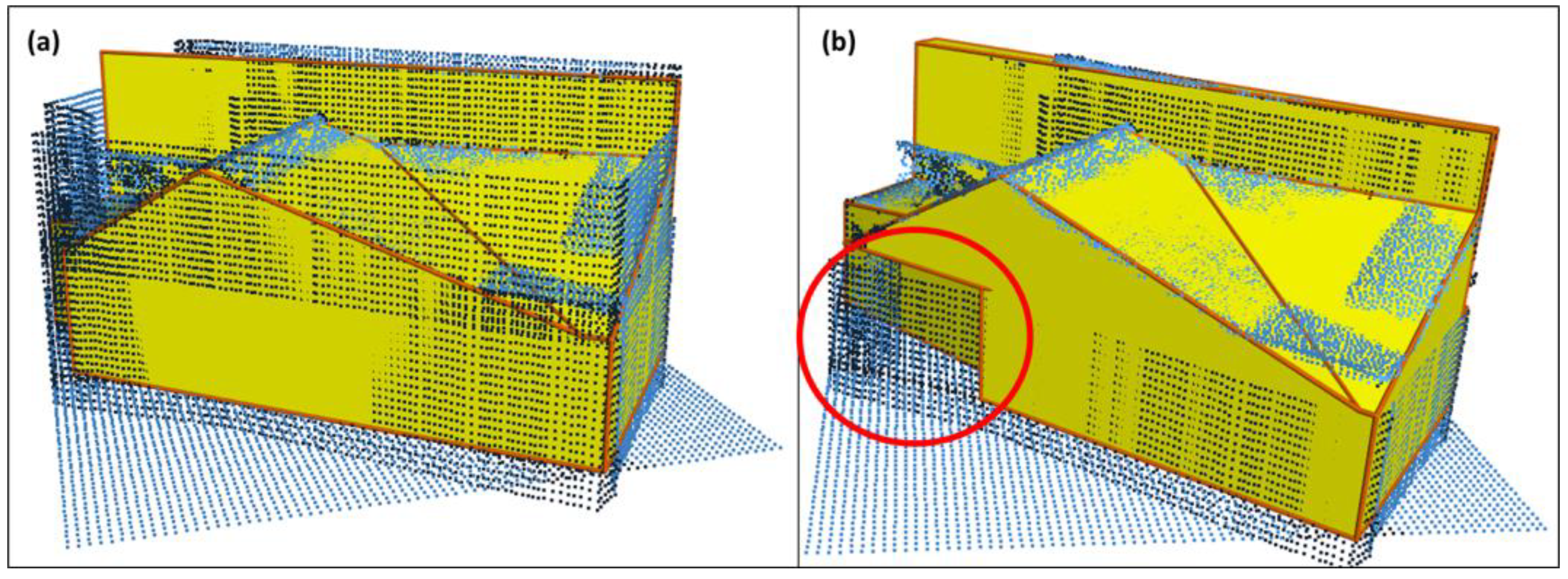
In order to obtain complete point clouds of individual buildings, the densification process was carried out by utilizing the roof boundary. The output of this process is shown in Figure 13. The densified point clouds of the exterior walls extended beyond the ceiling limit, which was generated from the maximum roof height (Figure 24a). This was necessary to anticipate potential issues that could arise if the densification of point clouds relied only on the minimum height of the ceiling during the modelling process. Such an approach could create gaps between the exterior walls, roofs, and grounds, which in turn may cause imperfections in the surface plane optimization. The imperfections caused by these gaps are illustrated with red circles in Figure 24b, where the generated model shows inconsistencies resulting from those modeling challenges.
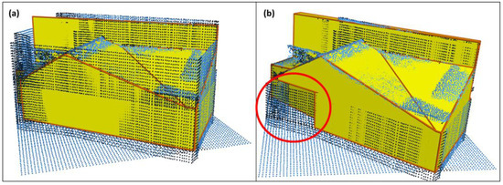
Figure 24.
Different results of the generated 3D building model due to gaps in the point clouds. (a) Generated 3D building model without gaps in point clouds. (b) Imperfect 3D building model generated with gaps in point clouds (Yellow solids represent the 3D building model, blue points represent the densified point clouds of the individual building, red circle shows imperfections of the surface plane optimization).
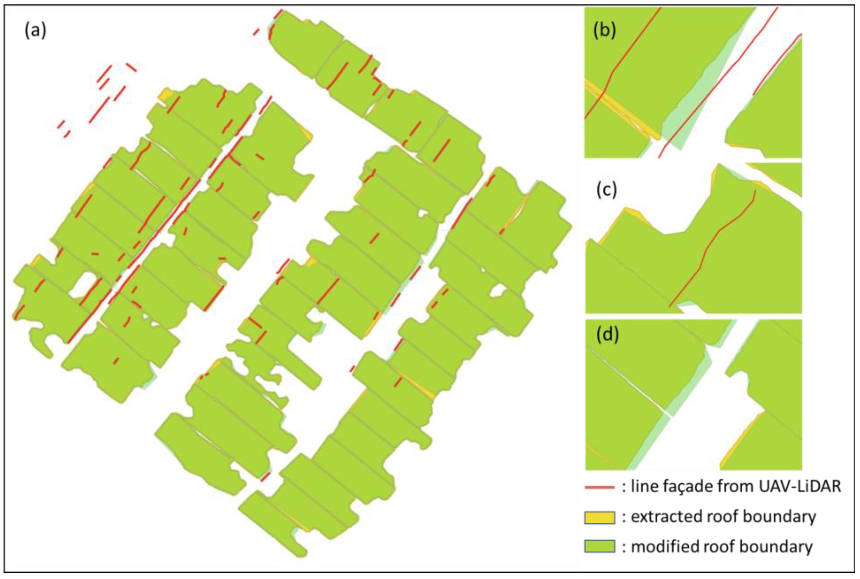
The previous stage generated a 3D building model at LOD 2.2 using a polyhedron data structure. To update this model with the exterior wall class from the UAV-LiDAR point clouds, the extracted roof boundary from the second phase of the modelling process was reused and modified using geometric orthogonality. The ‘body of the building’ was then reconstructed through densification of this modified boundary. Figure 25a illustrates the difference between the extracted roof boundary (yellow polygon), the modified boundary (green polygon), and the exterior wall lines derived from UAV-LiDAR (red line).
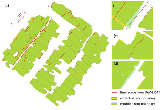
Figure 25.
(a) Overlay between the line façade from UAV-LiDAR and the original roof boundary. (a) Line façade from UAV-LiDAR, extracted and modified roof boundary. (b,c) the original roof boundary with short segments. (d) Formation of a smoother and more continuous roof edge.
Although the orthogonality process was able to shift roof boundary edges to better align with actual exterior wall lines, it had both advantages and drawbacks. For example, when the original roof boundary consisted of many short segments, the process did not perform effectively, as seen in Figure 25b,c. On the other hand, the orthogonality process can simplify geometry by eliminating redundant or colinear edges, resulting in a smoother roof boundary (Figure 25d). This updated roof boundary was then used to generate the refined 3D ‘body of the building’.
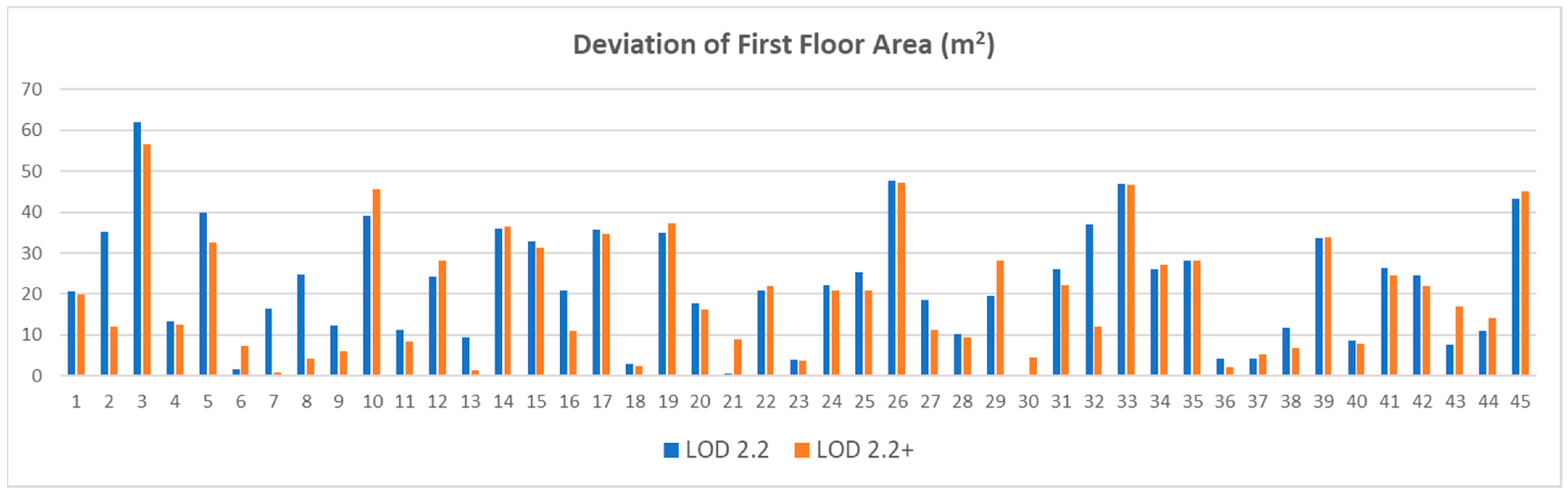
The refinement process improved the 3D building model by producing more realistic exterior walls compared to the original version. The deviation of floor area from the 3D building model LOD2.2 to LOD2.2+ was reduced from 24.688 m2 to 21.646 m2. This reduction indicates that the refinement from LOD2.2 to LOD2.2+ led to an improvement in area accuracy. Unfortunately, the exterior wall data from UAV-LiDAR only helped improve the first-floor area of the 3D building model by approximately ±3 m2. Even though the deviation in total floor area showed only a minor difference of about ±3 m2, the orthogonality concept can still support the updating of 3D building models using actual exterior wall data from other sources. The deviation of the first-floor area of the 3D models can be seen in Figure 26.
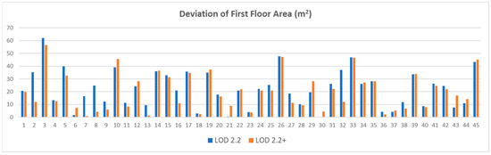
Figure 26.
First floor area deviation before and after update.
Moreover, the analysis for fiscal cadastre purposes was found to be necessary due to the urgent role of cadastre functions in Indonesia, as previously described in the research background. Based on the 3D property valuation framework by Yamani et al. (2021), which considers not only geometric attributes but also openings and sun exposure as important factors, 43% of the required valuation elements were provided by the products of this research [42]. In addition, Kara et al. (2023) conducted an experiment on 3D property valuation using 3D models to support taxation transparency [8]. The 3D building model developed in this research was able to provide 57% of the valuation elements identified by Kara et al. (2023). Table 2 shows the availability of 3D property valuation elements covered by the outputs of this research.
Table 2.
Availability of 3D property valuation elements, a product of this research.
Although this automatic workflow, along with the refinement process, produced a more detailed 3D building model using façade data from UAV-LiDAR, the algorithm still requires further research to address its limitations—particularly in the 3D modeling and refinement stages. Currently, the updated model can only be applied to the first floor of the 3D building model, which is based on a polyhedron data structure.
This research also focuses solely on the geometric aspects and the integration between 3D rights and 3D building models. The automatic workflow is limited to modeling non-overlapping rights spaces. 3D buildings are not generated if there are no associated rights, as the workflow relies on the integration of both models. Furthermore, the modeling may be inaccurate if the representation of legal boundaries is incorrect from the outset.
Another limitation of this research is that scalability has not yet been addressed. The case study is in a regular urban area with a small Area of Interest (AOI) and limited computational resources. Future research should consider a wider range of cases, such as irregular urban patterns, larger AOIs, and enhanced device capabilities.
Using a different data structure, such as GML, may result in more accurate modeling for upper floors, especially since densification results prior to modeling can help identify specific point cloud classes such as roofs, exterior walls, and building floors. The difference in data structures used for 3D building model reconstruction presents the next challenge in modelling. This classification supports more effective refinement, enabling façade updates not only on the first floor but also on upper levels, as required by LOD 3 modeling. Nevertheless, this study can provide new insights for updating building models that still use roof edges as the outer building walls, as is common in LOD2 models. This becomes even more relevant if the point cloud data representing exterior building walls is more complete, such as that obtained from terrestrial scanning.
A possible direction for future research is to integrate the refined 3D building model with a cadastral database using the LADM standard for 3D cadastre, as shown previously in Figure 5. LADM provides the data structure, while real-time processing offers speed and up-to-date information, which is very important to support dynamic land administration. Together, they complement each other in building a land administration system that is adaptive, responsive, and efficient in the digital era.
In addition, future work should explore the integration of 3D building models with Building Information Modeling (BIM), which can offer richer semantic and legal information about spatial units. Linking BIM with LADM and real-time processing would enhance the ability to manage legal and physical changes in buildings more dynamically and accurately, especially in complex urban environments.
6. Conclusions
This study presented an automated framework for constructing 3D cadastral models of 3D rights and buildings, leveraging ‘RAW’ data from UAV-LiDAR and minimizing the need for manual input. The framework consisted of a combination of algorithms applied in each stage. This research employed a combination of several algorithms; the key findings are as follows:
- The GMM technique proved useful for classifying noise from other classes in segmented point clouds of the roof class produced by the RF method.
- The ICP algorithm was beneficial for adjusting existing 2D parcels to new data without changing their geometric form and provided transformation parameters useful for further development.
- The region growing algorithm with specific parameters was effective in segmenting point clouds into individual roofs. Additionally, the roof boundary could be reused in the densification process to obtain complete point clouds for individual buildings.
- The orthogonality concept enabled the updating of 3D building models using exterior wall point clouds captured by UAV-LiDAR.
However, this research has several limitations. In the noise filtering stage, the roof-class segmented point clouds produced by RF were not only differentiated from other classes but also from noise within the roof class itself. In the 2D parcel adjustment stage, the RMSE was relatively high due to the wide range of deviation, suggesting that each parcel may require different transformation parameters. Further research is needed to improve accuracy in this area.
Moreover, the updated 3D building model in this study used a polyhedron data structure, which limited the refinement phase only to the first floor. As a result, the 3D model updates were not yet optimal. Further research should explore the use of alternative data structures to enhance the 3D building model refinement process. Also, by using another point cloud of the exterior walls of the building from other resources.
Supplementary Materials
The following supporting information: (1) Polygonal Surface Reconstruction-Polyfit_v1.5 by Nan & Wonka (2017) can be downloaded at: https://github.com/LiangliangNan/PolyFit/releases (accessed on 20 June 2024); (2) Point cloud processing and visualization-Easy3D-v2.5.3 by Nan & Wonka (2017) can be downloaded at: https://github.com/LiangliangNan/Easy3D/releases (accessed on 20 June 2024).
Author Contributions
Conceptualization, investigation, methodology, writing—original draft, Ratri Widyastuti; conceptualization, writing—original draft, resources, Deni Suwardhi; reviewing and editing, Irwan Meilano and Andri Hernandi; visualization, Juan Firdaus. All authors have read and agreed to the published version of the manuscript.
Funding
Contract number: PPMI-ITB-2024: 57B/IT1.C01/SK-TA/2024.
Data Availability Statement
Data are unavailable due to privacy.
Acknowledgments
We are grateful to Aditya Kurnia for helping us with some stages of data processing in this research.
Conflicts of Interest
The authors declare no conflicts of interest.
References
- Williamson, I.; Enemark, S.; Wallace, J.; Rajabifard, A. Land Administration for Sustainable Development, 1st ed.; ESRI Press Academic: Redlands, CA, USA, 2010. [Google Scholar]
- Dale, P.F.; Mclaughlin, J.D. Land Registration. In Land Administration System, 1st ed.; Oxford University Press: Oxford, UK, 1999. [Google Scholar]
- Rajabifard, A. 3D Cadastres and Beyond. In Proceedings of the 4th International Workshop on 3D Cadastres, Dubai, United Arab Emirates, 9 November 2014. [Google Scholar]
- Stoter, J. 3D Cadastre. Ph.D. Thesis, Delft University of Technology (TU Delft), Delft, The Netherlands, 2004. [Google Scholar]
- Oosterom, P.; Van Lemmen, C.; Thompson, R.; Janecka, K.; Zlatanova, S.; Kalantari, M. 3D Cadastres Best Practices, Chapter 3: 3D Cadastral Information Modelling. In FIG Congress; International Federation of Surveyors (FIG): Copenhagen, Denmark, 2018. [Google Scholar]
- Ying, S.; Guo, R.; Oosterom, P.; Van Stoter, J.; Li, L.; Van Oosterom, P.; Ledoux, H.; Peter, C.; Oosterom, V. Design and Development of a 3D Cadastral System Prototype based on the LADM and 3D Topology. In Proceedings of the 2nd International Workshop on 3D Cadastres 16, Delft, The Netherlands, 16–18 November 2011; Available online: https://www.researchgate.net/publication/228814769 (accessed on 25 June 2024).
- Rebong, F.R.; Meilano, I.; Sadarviana, V.; Hernandi, A.; Abdulharis, R.; Meilani, R. Strategy for the Conversion of 2D to 3D Cadastral Maps by Standardizing the Height Limit of Land Rights Space Based on Land Use/Land Cover. Land 2025, 14, 763. [Google Scholar] [CrossRef]
- Kara, A.; Oosterom, P.; Van Kathmann, R.; Lemmen, C. Visualisation and dissemination of 3D valuation units and groups—An LADM valuation information compliant prototype. Land Use Policy 2023, 132, 106829. [Google Scholar] [CrossRef]
- Lee, K.W.; Park, J.K. Comparison of UA- image and UAV-LiDAR for construction of 3D geospatial information. Sens. Mater. 2019, 31, 3327–3334. [Google Scholar] [CrossRef]
- Biljecki, F.; Ledoux, H.; Stoter, J. An improved LOD specification for 3D building models. Comput. Environ. Urban Syst. 2016, 59, 25–37. [Google Scholar] [CrossRef]
- Peters, R.; Dukai, B.; Vitalis, S.; Liempt, J.; Van Stoter, J. Automated 3D Reconstruction of LoD2 and LoD1 Models for All 10 Million Buildings of the Netherlands. Photogramm. Eng. Remote Sens. 2022, 88, 165–170. [Google Scholar] [CrossRef]
- Murtiyoso, A.; Veriandi, M.; Suwardhi, D.; Soeksmantono, B.; Harto, A. Automatic Workflow for Roof Extraction and Generation of 3D CityGML Models from Low-Cost UAV-Image-Derived Point Clouds. ISPRS Int. J. Geo-Inf. 2020, 9, 743. [Google Scholar] [CrossRef]
- Ross, L.; Buyuksalih, G.; Buhur, S. 3D City Modelling for Planning Activities, Case Study: Haydarpasa Train Station, Haydarpasa Port and Surrounding Backside Zones, Istanbul. In Proceedings of the ISPRS Hannover Workshop, Hannover, Germany, 2–5 June 2009; Available online: https://www.researchgate.net/publication/237442235 (accessed on 11 January 2023).
- Šafář, V.; Potůčková, M.; Karas, J.; Tlustý, J.; Štefanová, E.; Jančovič, M.; Žofková, D.C. The Use of UAV in Cadastral Mapping of the Czech Republic. ISPRS Int. J. Geo-Inf. 2021, 10, 380. [Google Scholar] [CrossRef]
- Dragomir, L.O.; Popescu, C.A.; Herbei, M.V.; Popescu, G.; Herbei, R.C.; Salagean, T.; Bruma, S.; Sabou, C.; Sestras, P. Enhancing Conventional Land Surveying for Cadastral Documentation in Romania with UAV-Photogrammetry and SLAM. Remote Sens. 2025, 17, 2113. [Google Scholar] [CrossRef]
- Manzini, T.; Perali, P.; Karnik, R.; Godbole, M.; Abdullah, H.; Murphy, R. Non-Uniform Spatial Alignment Errors in sUAS Imagery from Wide-Area Disasters. arXiv 2025, arXiv:2405.06593. Available online: http://arxiv.org/abs/2405.06593 (accessed on 21 July 2025).
- Kitsakis, D.; Paasch, J.M.; Paulsson, J. 3D Cadastres Best Practices, Chapter 1: Legal Foundations. In FIG Congress; International Federation of Surveyors (FIG): Copenhagen, Denmark, 2018. [Google Scholar]
- Strang, G. Introduction to Linear Algebra, 4th ed.; Wellesley-Cambridge Press: Wellesley, MA, USA, 2003. [Google Scholar]
- Satwika, I.P.; Suwardhi, D.; Hernandi, A.; Ratrianto, L.; Masykur, M. Parcel Matching based on Point Feature Using Block Adjustment. In Proceedings of the The International Conference and South East Asian Surveyor Congress (SEASC), Bandung, Indonesia, 2–4. August 2022; Volume 40124. Available online: https://www.researchgate.net/publication/365359248 (accessed on 24 July 2024).
- Besl, P.J.; McKay, N.D. A method for registration of 3-D shapes. IEEE Trans. Pattern Anal. Mach. Intell. 1992, 14, 239–256. [Google Scholar] [CrossRef]
- Yi, C.; Zhang, Y.; Wu, Q.; Xu, Y.; Remil, O.; Wei, M.; Wang, J. Urban building reconstruction from raw LiDAR point data. CAD Comput. Aided Des. 2017, 93, 1–14. [Google Scholar] [CrossRef]
- Nan, L.; Wonka, P. PolyFit: Polygonal Surface Reconstruction from Point Clouds. In Proceedings of the IEEE International Conference on Computer Vision, Venice, Italy, 22–29 October 2017; pp. 2353–2361. [Google Scholar]
- Chen, H.-P.; Chang, K.-T.; Liu, J.-K.; Author, C. Strip Adjustment of Airborne LiDAR Data Using Ground Points. In Proceedings of the Asian Conference on Remote Sensing, Pattaya, Thailand, 26–30 November 2012; p. 3282. [Google Scholar]
- Carrilho, A.C.; Galo, M.; Dos Santos, R.C. Statistical outlier detection method for airborne LiDAR data. Remote Sens. Spat. Inf. Sci. ISPRS Arch. 2018, 42, 87–92. [Google Scholar] [CrossRef]
- Zeybek, M.; Şanlıoğlu, İ. Point cloud filtering on UAV-based point cloud. Meas. J. Int. Meas. Confed. 2019, 133, 99–111. [Google Scholar] [CrossRef]
- Widyastuti, R.; Suwardhi, D.; Meilano, I.; Hernandi, A.; Putri, N.S.E.; Saptari, A.Y.; Sudarman. Performance Analysis of Random Forest Algorithm in Automatic Building Segmentation with Limited Data. ISPRS Int. J. Geo-Inf. 2024, 13, 235. [Google Scholar] [CrossRef]
- Bulut, V. Classifying Surface Points Based on Developability Using Machine Learning. Eur. J. Sci. Technol. 2022, 171–176. [Google Scholar] [CrossRef]
- Grilli, E.; Poux, F.; Remondino, F. Unsupervised object-based clustering in support of supervised point-based 3D point cloud classification. Int. Arch. Photogramm. Remote Sens. Spat. Inf. Sci. ISPRS Arch. 2021, 43, 471–478. [Google Scholar] [CrossRef]
- Han, X.F.; Jin, J.S.; Wang, M.J.; Jiang, W.; Gao, L.; Xiao, L. A review of algorithms for filtering the 3D point cloud. Signal Process. Image Commun. 2017, 57, 103–112. [Google Scholar] [CrossRef]
- Patel, E.; Kushwaha, D.S. Clustering Cloud Workloads: K-Means vs Gaussian Mixture Model. Procedia Comput. Sci. 2020, 171, 158–167. [Google Scholar] [CrossRef]
- Kang, C.; Wang, F.; Zong, M.; Cheng, Y.; Lu, T. Research on Improved Region Growing Point Cloud Algorithm. In Proceedings of the International Conference on Geomatics in the Big Data Era (ICGBD), Guilin, China, 15–17 November 2019; Volume 42, pp. 153–157. [Google Scholar] [CrossRef]
- Laraseta, L. Permasalahan Atap Bangunan Gedung dan Solusinya. J. Infrastruktur. 2022. Available online: https://simantu.pu.go.id/content/?id=5305 (accessed on 23 September 2024).
- Yahya, Z.; Rahmat, R.W.; Khalid, F.; Rizaan, A.; Rizal, A. A Concave Hull Based Algorithm for Object Shape Reconstruction. Int. J. Inf. Technol. Comput. Sci. 2017, 9, 1–9. [Google Scholar] [CrossRef]
- Safitri, S. The Implementation of Land Administration Domain Model (LADM and 3D Cadastre on Cadastral Data Management in Indonesia; Institut Teknologi Bandung: Bandung, Indonesia, 2014. [Google Scholar]
- ISO 19152:2012; Geographic Information-Land Administration Domain Model (LADM). ISO: Geneva, Switzerland, 2012. Available online: www.iso.org (accessed on 20 May 2023).
- Souza, G.H.; Amorim, A. LiDAR Data Integration for 3D Cadastre: Some Experiences from Brazil LiDAR Data Integration for 3D CADASTRE: Some Experiencies from Brazil. In Proceedings of the FIG Working Week, Roma, Italy, 6–10 May 2012; pp. 1–15. [Google Scholar]
- Oosterom, P.; Van Stoter, J.; Lemmen, C.; Van Oosterom, P. Modelling of 3D Cadastral Systems. 2005. Available online: https://www.researchgate.net/publication/267956219 (accessed on 15 March 2025).
- Atazadeh, B.; Kalantari, M.; Rajabifard, A.; Ho, S. Modelling building ownership boundaries within BIM environment: A case study in Victoria, Australia. Comput. Environ. Urban Syst. 2017, 61, 24–38. [Google Scholar] [CrossRef]
- Hernandi, A.; Suwardhi, D.; Widyastuti, R.; Handayani, A.P.; Harpiandi, A. Utilization of LADM for Smart Village Development in Indonesia. In Proceedings of the FIG Working Week, Amsterdam, The Netherlands, 10–14 May 2020. [Google Scholar]
- Grilli, E.; Menna, F.; Remondino, F. A review of point clouds segmentation and classification algorithms. Int. Arch. Photogramm. Remote Sens. Spat. Inf. Sci. ISPRS Arch. 2017, 42, 339–344. [Google Scholar] [CrossRef]
- Costantino, D.; Pepe, M.; Angelinii, M.G. Evaluation of reflectance for building materials classification with terrestrial laser scanner radiation. Acta Polytech. 2021, 61, 174–198. [Google Scholar] [CrossRef]
- Yamani, S.E.; Hajji, R.; Nys, G.A.; Ettarid, M.; Billen, R. 3D variables requirements for property valuation modeling based on the integration of bim and cim. Sustainability 2021, 13, 2814. [Google Scholar] [CrossRef]


Disclaimer/Publisher’s Note: The statements, opinions and data contained in all publications are solely those of the individual author(s) and contributor(s) and not of MDPI and/or the editor(s). MDPI and/or the editor(s) disclaim responsibility for any injury to people or property resulting from any ideas, methods, instructions or products referred to in the content. |
© 2025 by the authors. Published by MDPI on behalf of the International Society for Photogrammetry and Remote Sensing. Licensee MDPI, Basel, Switzerland. This article is an open access article distributed under the terms and conditions of the Creative Commons Attribution (CC BY) license (https://creativecommons.org/licenses/by/4.0/).