Article

Activity Spaces in Multimodal Transportation Networks: A Nonlinear and Spatial Analysis Perspective

1
College of Architecture and Urban Planning, Tongji University, Shanghai 200092, China
2
Faculty of Transportation Engineering, Kunming University of Science and Technology, Kunming 650032, China
3
Department of Transportation Engineering, Tongji Zhejiang College, Jiaxing 314051, China
*
Author to whom correspondence should be addressed.
ISPRS Int. J. Geo-Inf. 2025, 14(8), 281; https://doi.org/10.3390/ijgi14080281
Submission received: 7 May 2025 / Revised: 3 July 2025 / Accepted: 14 July 2025 / Published: 22 July 2025

Abstract

Activity space offers a valuable perspective for analyzing urban travel behavior and evaluating the performance of transportation systems in increasingly complex urban environments. However, the research on measuring activity spaces in multimodal transportation contexts remains limited. This study investigates multimodal transportation activity spaces in Hangzhou using 2023 smart card data. Multimodal travel chains are extracted, and residents’ activity spaces are quantified using 95% confidence ellipses. By applying the XGBoost and GeoShapley models, this study reveals the nonlinear effects and geospatial heterogeneity in how built environment and socioeconomic factors influence activity spaces. The key findings show that the distance to the nearest metro station, commercial POIs, and GDP significantly shape activity spaces through nonlinear relationships. Moreover, the interaction between the distance to the nearest metro station and geographical location generates pronounced geospatial effects. The results highlight the importance of multimodal integration in urban transport planning and provide empirical insights for enhancing system efficiency and sustainability.

1. Introduction

With the continuous advancement of global urbanization, urban transportation systems are facing increasingly complex challenges, which have become major constraints on sustainable urban development and the improvement of residents’ quality of life. Challenges such as traffic congestion, environmental pollution, and energy consumption impose substantial pressures on cities. Therefore, improving the efficiency and sustainability of urban transportation systems has become a pressing concern in the fields of urban planning and transportation management [1].
Activity space, as a spatial representation of individual mobility and accessibility, is a widely used concept in transportation planning, urban studies, and public health research [2]. It reflects the geographical area within which individuals conduct their daily activities and travel over a specific period, capturing the dynamic interaction between human behavior and the built environment [3]. Through the lens of activity space, researchers can analyze the spatial disparities in accessibility, identify patterns of social exclusion, evaluate transport equity, and understand how urban form and infrastructure shape human mobility [4]. In the era of people-oriented smart city development, analyzing individuals’ spatiotemporal behavior from an activity space perspective has become increasingly important. However, traditional analyses of activity space often rely on single-mode transportation data (e.g., bus [5], private car [6]), which fail to capture the complexity of mobility patterns in multimodal transportation environments [7]. With growing urban complexity and increasingly diverse travel demands, individuals are more likely to combine multiple modes—such as walking, cycling, ride-hailing, and public transit—to meet their mobility needs [6,8,9,10]. Consequently, single-mode activity space analysis can no longer fully address residents’ mobility needs, necessitating a comprehensive consideration of multimodal transportation activity spaces.
The measurement of multimodal transportation activity spaces requires the holistic analysis of geospatial distributions, usage frequencies, and interrelationships among different transportation modes [11]. This involves not only the physical layout of transportation infrastructure but also the transfer efficiency and convenience between modes. Recent advancements in big data and geographic information systems (GIS) have enabled more precise spatiotemporal analyses of travel behavior [12]. Nevertheless, most existing studies remain focused on single-mode travel and offer limited insights into the complexity and dynamics of multimodal transportation systems. Moreover, the mechanisms through which urban environmental characteristics, socioeconomic attributes, and transportation infrastructure shape multimodal activity spaces remain insufficiently understood. In particular, the nonlinear relationships and crossmodal interdependencies that shape multimodal activity spaces are underexplored. Therefore, a deeper investigation into the measurement methods and influencing mechanisms of multimodal transportation activity spaces is of both theoretical and practical importance for formulating scientific transportation policies and planning.
This study aims to explore the characteristics of multimodal transportation activity spaces and their impact mechanisms on urban development through innovative measurement methods and analytical models, with a particular focus on nonlinear relationships and geospatial effects. By conducting a comprehensive analysis of multiple travel modes, we expect to provide new insights and tools for urban transportation planning, facilitating the construction of more efficient, sustainable, and inclusive urban transportation systems. The main contributions of this study are as follows: (1) We integrate bus and metro smart card data from Hangzhou, China, to extract residents’ multimodal travel chains, capturing origin–destination pairs, travel times, and transportation modes, thereby establishing a robust empirical foundation for subsequent analysis. (2) We incorporate both spatial and temporal dimensions to construct 95% confidence ellipses based on grid-level travel patterns, which delineate the spatial extent of multimodal activity spaces. (3) We identified key built environment and socioeconomic variables (e.g., population density, road networks, land use) and employ the XGBoost model to assess their influence. The GeoShapley interpretability framework is further applied to uncover the nonlinear effects and spatially varying mechanisms shaping activity space dynamics.
The remainder of the paper is organized as follows: Section 2 reviews the literature related to this study; Section 3 introduces the model methods for measuring multimodal transportation activity space and its influencing factors; Section 4 presents the study area and modeling variables; Section 5 discusses the results; and Section 6 includes conclusions, policy implications, limitations, and research prospects.

2. Literature Review

2.1. Conceptualization and Measurement of Activity Space

Activity space has emerged as a key concept in behavioral geography, representing individuals’ geospatial patterns of daily activities and interactions with urban environments [13]. It transcends physical urban spaces by emphasizing personal behaviors and the formation of “invisible spaces” through urban facility utilization and social participation [14]. Rooted in time–geography principles, activity space research focuses on time–space budgets and individual constraints [13]. Studies have revealed significant differences in activity space characteristics among residents of different neighborhood types, highlighting socio-spatial segregation in terms of geospatial extensity, intensity, and exclusivity [15]. Contemporary methodologies employ GPS data and GIS analysis to precisely measure individual activity spaces, examining factors influencing urban space utilization and addressing challenges from rapid suburbanization such as prolonged commutes and job–housing mismatches [16]. These approaches provide critical insights into urban social dynamics and inform planning policy decisions.
The conceptual foundation of activity space measurement originates from the time–geographic notion of “space-time prisms” [17]. Early researchers utilized two-dimensional projections of space–time prisms to interpret travel behaviors, primarily describing individuals’ potential activity spaces through accessible geospatial ranges under specific spatiotemporal constraints [18]. With the advancements in accessibility research, scholars introduced empirical activity space measurements to characterize the interactions between individual travel behaviors and urban spaces [19].
Newsome et al. [20] pioneered the use of elliptical models—which apply standard deviational ellipses to statistically summarize the spatial distribution of activity locations—to construct activity spaces within time–geography frameworks, emphasizing commuters’ spatially constrained activity structures. Building on this, Buliung & Kanaroglou [21] incorporated non-work activity locations into convex polygon models using household members’ daily activity anchors, achieving more precise depictions of travelers’ accessible spaces.
Drawing from Golledge’s geospatial cognition theory [22], Schönfelder & Axhausen [23] proposed path buffer zones to represent activity spaces by correlating road network paths with surrounding areas, thereby approximating travelers’ actual activity ranges. When characterizing residents’ activity–travel behaviors, temporal allocation proves equally critical as geospatial distance. Zhou et al. [24] introduced the Functional Crucial Network Location (FCNL) concept, analyzing spatiotemporal travel patterns using taxi trajectory data. Li et al. [25] applied network analysis techniques including PageRank and community detection to identify hub stations and community structures in public transit networks. Wang et al. [26] developed novel visualization methods using time–statistical maps to represent transportation accessibility dynamics, incorporating metrics like Shortest Railway Travel Time (STRT) and Spatiotemporal Conversion Parameters (STCPs). With advancements in 3D GIS visualization, researchers have achieved three-dimensional representations of residents’ spatiotemporal travel ranges. This integration overcomes the limitations of 2D representations by effectively conveying 3D geospatial information [12]. For instance, Yu & Shaw [27] designed a 3D spatiotemporal GIS framework that adapts space–time prism concepts to visualize and analyze potential human activities in both physical and virtual spaces. The key articles are summarized in Table 1.

2.2. Activity Space–Travel Behavior Research

Activity-based travel behavior analysis has gained prominence since the 1970s, focusing on individual activity participation and derived travel demands [28,29]. These approaches overcome the limitations of traditional four-step models by incorporating spatiotemporal constraints and daily activity patterns [30]. As the representations of individuals’ directly experienced locations, activity spaces prove crucial for understanding travel behaviors and urban structures.
Studies demonstrate that built environment characteristics—particularly transportation facility density and accessibility—significantly influence activity space dimensions [30,31]. Socioeconomic factors including occupational roles and income levels also play substantial roles [32]. For example, Duan et al. [30] identified facility density, accessibility, location attributes, housing conditions, and marital status as key factors exhibiting diminishing marginal effects and threshold characteristics. Chen & Akar [33] found that low-income populations in Greater Cleveland faced no accessibility disadvantages, with urbanized neighborhoods enhancing accessibility. Conversely, Tao et al. [34] observed persistent activity space disparities among income groups in Hong Kong despite urban development. Sharmeen & Houston [35] reported that land use mix significantly predicted activity space size in Dhaka, with less diverse areas exhibiting larger activity spaces. Some scholars argue that built environment factors exert a greater influence on residents’ daily activity space patterns than socioeconomic attributes [36]. These findings underscore the complex interplay between built environments, sociodemographics, and activity spaces across urban contexts.
Methodologically, most activity space–travel behavior studies assume linear relationships between explanatory and dependent variables. For instance, Chen & Akar [37] applied OLS regression to examine neighborhood type and sociodemographic impacts on activity spaces. Similarly, Tana et al. [38] employed linear regression for a comparative analysis of suburban activity spaces in Beijing and Chicago, identifying context-specific influencing factors.
Recent studies increasingly focus on nonlinear relationships using machine learning techniques like random forest [39], GBDT [40], GBRT [41], and LightGBM. Duan et al. [30] developed random forest models with partial dependence plots to explore the nonlinear impacts of built environment and sociodemographic factors, confirming the existence of nonlinear mechanisms despite not addressing multimodal contexts.
In summary, as a core concept in behavioral geography, activity space captures individuals’ geospatial interaction patterns with urban environments. The existing research highlights transportation infrastructure density and accessibility as critical built environment determinants of activity space size, complemented by socioeconomic influences. However, the predominant focus on single transportation modes limits the comprehensive understanding of multimodal systems.
Existing studies predominantly concentrate on single-mode transportation activity space research, lacking the comprehensive measurement and evaluation of multimodal transportation systems. Particularly under rapid urban development, the diversification of residents’ travel modes has rendered single-mode research insufficient to address practical demands. Although emerging research has begun to explore the nonlinear relationships between activity spaces and travel behaviors, the effective revelation of nonlinear impacts and geospatial effects among multimodal transportation activity spaces remains an underexplored domain.
This research aims to address these gaps by investigating the characteristics and influencing mechanisms of multimodal transportation activity spaces through innovative measurement methods and analytical models. Specifically, this study will holistically consider multiple transportation modes, revealing the interrelationships between different modes in multimodal systems through the integrated analysis of bus and metro travel chains. This approach provides novel perspectives for urban transportation planning. Subsequently, the XGBoost and GeoShapley models will be employed to deeply analyze the nonlinear factors and geospatial effects influencing multimodal transportation activity spaces, thereby enhancing the understanding of the complex impacts different transportation modes exert on residents’ travel behaviors.

3. Methodology

3.1. Extraction of Complete Travel Chains

A travel chain refers to the complete travel process of a passenger from their true origin to their final destination. It includes the access leg to the first transit station, the main travel segments on public transportation (passing through nodes like bus stops or metro stations), any transfers, and the final egress leg from the last station to the destination. The travel modes used for access and egress legs, such as walking, are critical components of the overall journey. A travel chain can be single mode or multimodal (here “mode” refers to the transportation methods that a passenger may use during the journey). This paper uses the extracted travel chains to measure the activity space of multimodal transportation users, which helps to explore the multimodal travel characteristics of passengers.
In public transportation travel, a complete OD (origin–destination) travel chain typically includes the following processes: departure preparation, waiting for the metro (or bus), boarding, riding, transferring, alighting, arriving at the destination, and ending the trip. By analyzing the behavioral changes in passengers in a complete OD travel chain, it can be understood that the total travel time of passengers is mainly composed of five time elements: walking time before and after entering the station, waiting time, riding time, transfer time, and walking time after arriving at the station. This paper mainly studies the multimodal travel mode of transfer passengers; compared with OD trips without transfers, it mainly considers the walking time during transfers and the waiting time at transfer stations.
The research data used in this study were obtained from one week of Integrated Circuit (IC) card transaction records in Hangzhou, covering the period from 1 November to 7 November 2023. IC cards—commonly referred to as public transit smart cards—electronically record each passenger transaction, including card ID, timestamp, and boarding location when entering the bus or metro system. Based on the above overview of urban public transport passenger travel time and under the condition of obtained IC card data, the passenger travel time for non-transfer routes Tod1 and transfer-required routes Todc can be calculated using the following formulas:
T od 1 = T d 1 T o 1
T o d c = i = 1 n T o d 1 + T o d 2 + + T od i + T c
T c = i n T o 2 T d 1 + T o 3 T d 2 + + T o i T d ( i 1 )
T i = T o i T d ( i 1 )
In the above formulas, Tod1 represents the travel time for passengers on non-transfer routes, Todc represents the travel time for passengers on transfer-required routes, Tc represents the total time during transfers, and Ti represents the time value of a single transfer. Ti can be obtained from filtered IC card data. However, in the above formulas, the variable Ti may include not only the walking and waiting time during transfers but also the time spent on non-transfer-related activities near the station, which could compromise the accuracy of the results. For instance, a passenger might spend 40 min dining during the transfer interval. It is therefore necessary to evaluate the duration of Ti to determine whether it represents a continuous transfer.
If the duration Ti between two or more boarding events (transfers) is large, it indicates that the passenger engaged in activities other than commuting near the intermediate station, and thus it cannot be regarded as continuous transfer behavior. Therefore, the value of Ti should not be too long. For the obtained IC card data and different transfer behaviors, we need to set a corresponding range value for Ti, i.e., a time threshold. In the study data of this paper, we denote the bus travel mode as B and the metro travel mode as R. Through data analysis, this paper sets the time thresholds for the three transfer behaviors of B-B, B-R, and R-B. First, all records with transfer intervals within 30 min are filtered from the data, and for these filtered records, the time difference for each transfer is calculated, i.e., the interval from the end of one boarding to the beginning of the next boarding. Then, these time differences are put into a set, and the 95th percentile of this set is calculated [42]. Finally, this 95th percentile is set as the time threshold for transfers, meaning that an effective transfer should be completed within this time threshold.
The time threshold settings for these three transfer behaviors are shown in Figure 1.
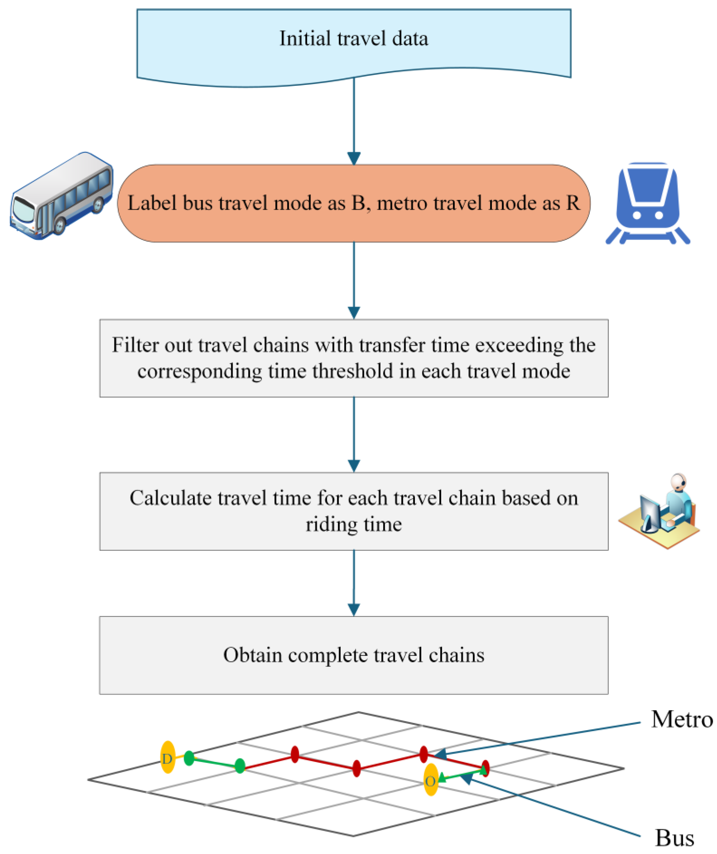
Based on the setting of the time threshold, the travel chains with transfer times exceeding the corresponding threshold are eliminated. Then, the travel chains are summarized according to the travel mode to obtain the initial complete travel chains. The travel time of each travel chain is calculated by subtracting the initial departure time from the final arrival time in the travel chain.
The flowchart for processing the initial travel data is shown in Figure 2.

3.2. Measurement and Analysis of Multimodal Transportation Activity Space

This paper is based on Hangzhou’s bus and metro card swiping data (see data sample in Section 4.1). By conducting an in-depth analysis of the B-R travel chain data in each grid of the study area, a confidence ellipse is constructed. The range of this confidence ellipse is defined as the transportation activity space of that grid area. In transportation research, the confidence ellipse is a widely used statistical method to characterize the geographic distribution of a set of points [43,44]. It effectively summarizes the central tendency, dispersion, and orientation of travel destinations. Conceptually, the ellipse is constructed by first calculating the mean center (i.e., the average x and y coordinates) of all destination points originating from a specific grid. Then, the standard deviation of these points is calculated along two perpendicular axes—the major and minor axes—which define the ellipse’s size and orientation. The size of the ellipse directly represents the spatial extent of the activity space: a larger ellipse indicates that residents travel over a wider area. In this study, we adopt the 95% confidence ellipse, which is standard practice to capture the vast majority of activity locations for each group. To conduct the spatial analysis, the study area within Hangzhou’s Ring Expressway was divided into a grid of 1 km × 1 km cells. These grids serve as the fundamental spatial unit of analysis. Based on the travel chain data originating from each grid, a confidence ellipse is constructed to represent the activity space of residents associated with that grid. To determine the activity space of residents using multimodal transportation within Hangzhou’s Ring Expressway, it is first necessary to understand how the values in the ellipse are calculated from geographic data. The following are the relevant formulas for the ellipse:
S D E x = i = 1 n   x i X 2 n
S D E y = i = 1 n     y i Y 2 n
t a n θ = i = 1 n     x ~ i 2 i = 1 n     y ˜ 2 + i = 1 n     x ~ i 2 i = 1 n     y ˜ 2 2 + 4 i = 1 n     x ~ i y ˜ 2 2 i = 1 n     x ~ i y ˜
σ x = i = 1 n     x ˜ i c o s θ y ˜ i s i n θ 2 n
σ y = i = 1 n     x ~ i s i n θ y ˜ i c o s θ 2 n
In the formulas, S D E x , S D E y represent the standard distances along the x-axis and y-axis, respectively; x i ,   y i denote the coordinates of each element i involved in the trip chain’s origin and its corresponding destination within the grid region; n represents the number of these origin elements; the ellipse is centered on the mean center ( x , y ) of the destination points; θ represents the rotation angle of the ellipse, meaning the long axis of the ellipse rotates counterclockwise from the north direction; x ˜ i , y ˜ i denote the deviation of each point’s coordinates x i , y i from the mean center of the point cluster; t a n θ is the orientation of the standard deviation ellipse; and σ x , σ y represent the standard deviations along the x-axis and y-axis, which correspond to the semi-major axis and semi-minor axis, respectively.
By determining the centroid position of the standard deviation ellipse in the activity space, the rotation angle of the ellipse, the values of the semi-major axis, and the semi-minor axis, the elliptical equation for each grid is obtained as follows:
X σ x 2 + Y σ y 2 = S 2
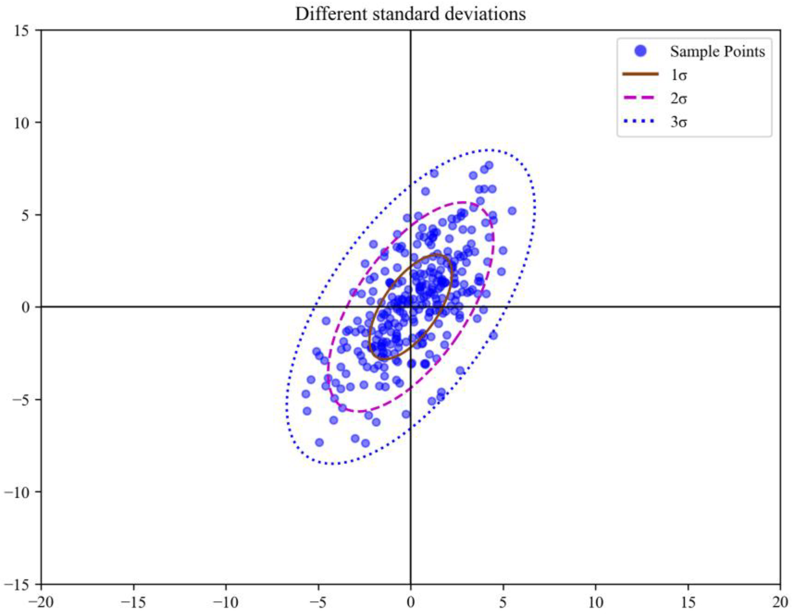
where S corresponds to the confidence level of the confidence ellipse. The schematic diagram for constructing the confidence ellipse is shown in Figure 3. The legend entries 1σ, 2σ, and 3σ denote standard deviational ellipses corresponding to one, two, and three standard deviations from the mean center of the data points, respectively. The Greek letter σ (sigma) represents standard deviation, a statistical measure of the dispersion of data around the mean.

3.3. XGBoost

XGBoost (Extreme Gradient Boosting) is a highly efficient and scalable implementation of gradient boosting that has gained widespread popularity in various scientific and industrial applications. It is particularly renowned for its ability to handle large-scale datasets and deliver state-of-the-art predictive performance. In this paper, the XGBoost model is used to explore the nonlinear influence of residents’ multimodal public transportation activity space. The specific model formula is in Appendix A.

3.4. GeoShapley

The traditional Shapley value calculation originates from cooperative game theory and is used to fairly allocate the contributions of participants in a cooperative game. When applied to machine learning models, the Shapley value is used to measure the contribution of each feature to the model’s prediction. The following is the calculation process for the Shapley value.
For a feature j , the formula for calculating its Shapley value ϕ j is as follows:
ϕ j = S N { j }   | S | ! ( p | S | 1 ) ! p ! [ f ( S { j } ) f ( S ) ]
where p is the total number of features, f ( S ) is the model prediction using the features in set S , and f ( S { j } ) is the model prediction after including feature j .
GeoShapley extends the traditional Shapley value framework to account for geospatial features as joint players in model interpretation [45]. This approach is particularly useful for models like XGBoost, where geospatial features significantly influence predictions.
GeoShapley value calculation: The GeoShapley value for a set of location features, denoted as ϕ G E O , is calculated by considering these features as a single joint player. The formula is as follows:
ϕ G E O = S N { G E O }   | S | ! ( p | S | g ) ! ( p g + 1 ) ! [ f ( S { G E O } ) f ( S ) ]
where   p is the total number of features, g is the number of location features, S is a subset of all features excluding the location features, f ( S ) is the model prediction using features in S , and f ( S { G E O } ) is the model prediction with the location features included. Here, GEO represents the geographic location of the target variable, usually the x and y values in the UTM coordinate system.
Interaction effect: The interaction between location features and a non-location feature X j is captured by Equation (12).
ϕ G E O , j = S M G E O , j   | S | ! ( p | S | g 1 ) ! ( p g + 1 ) ! [ f ( S { G E O , j } ) f ( S { G E O } ) f ( S { j } ) + f ( S ) ]
This measures how the presence of location features modifies the contribution of X j , reflecting spatially varying effects.
Comprehensive model interpretation: The total prediction for an observation can be decomposed as shown in Equation (13).
y ˆ = ϕ 0 + ϕ G E O + j = 1 p   ϕ j + j = 1 p   ϕ G E O , j
where ϕ 0 is a base value representing the average prediction, ϕ GEO   captures the intrinsic location effect, ϕ j represents the contribution of each non-location feature, and ϕ G E O , j accounts for geospatial interactions.
GeoShapley thus provides a detailed breakdown of how geospatial and non-spatial features contribute to model predictions, offering insights into the geospatial dynamics within XGBoost models.

4. Data and Variables

4.1. Study Area and Data Sources

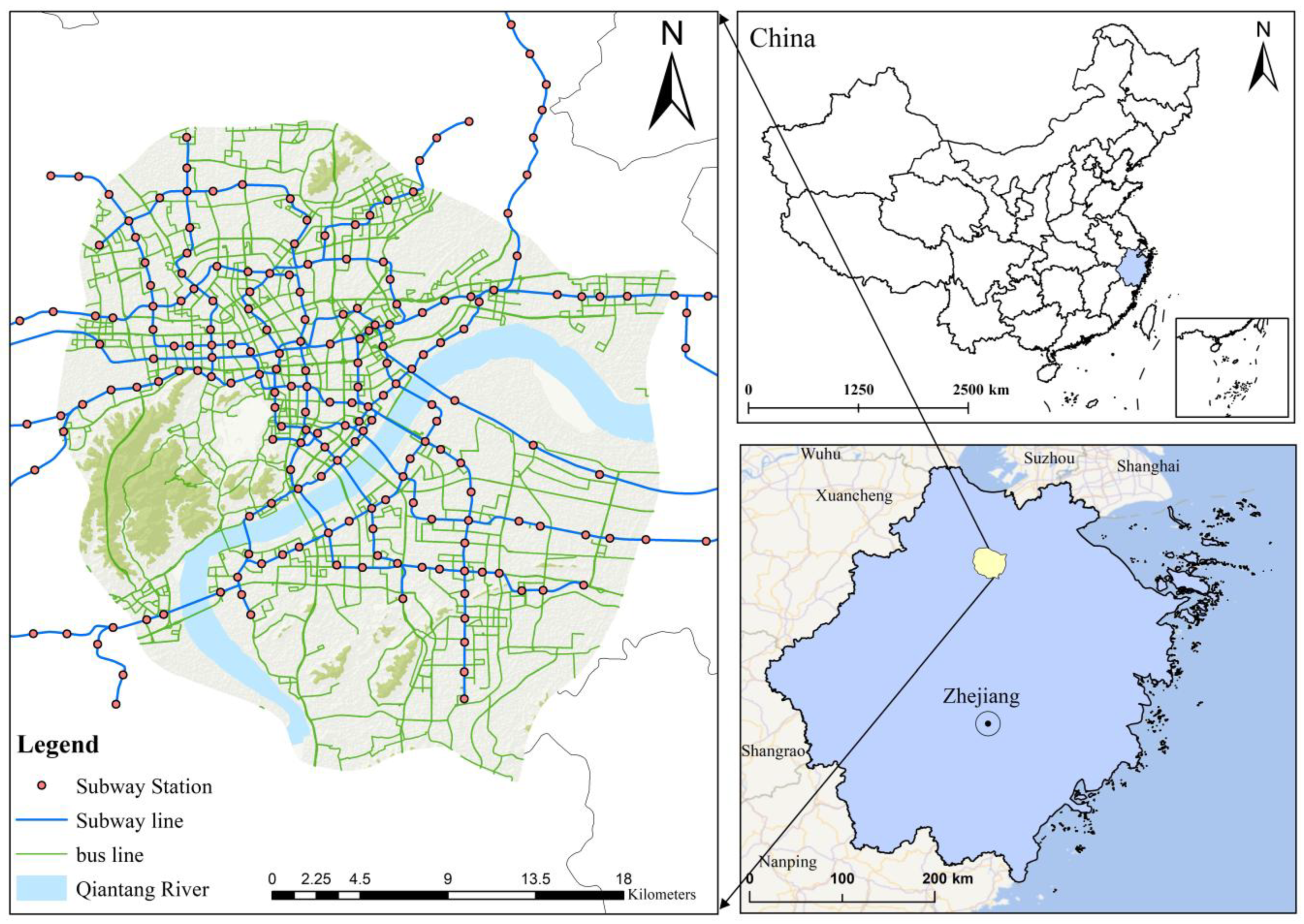
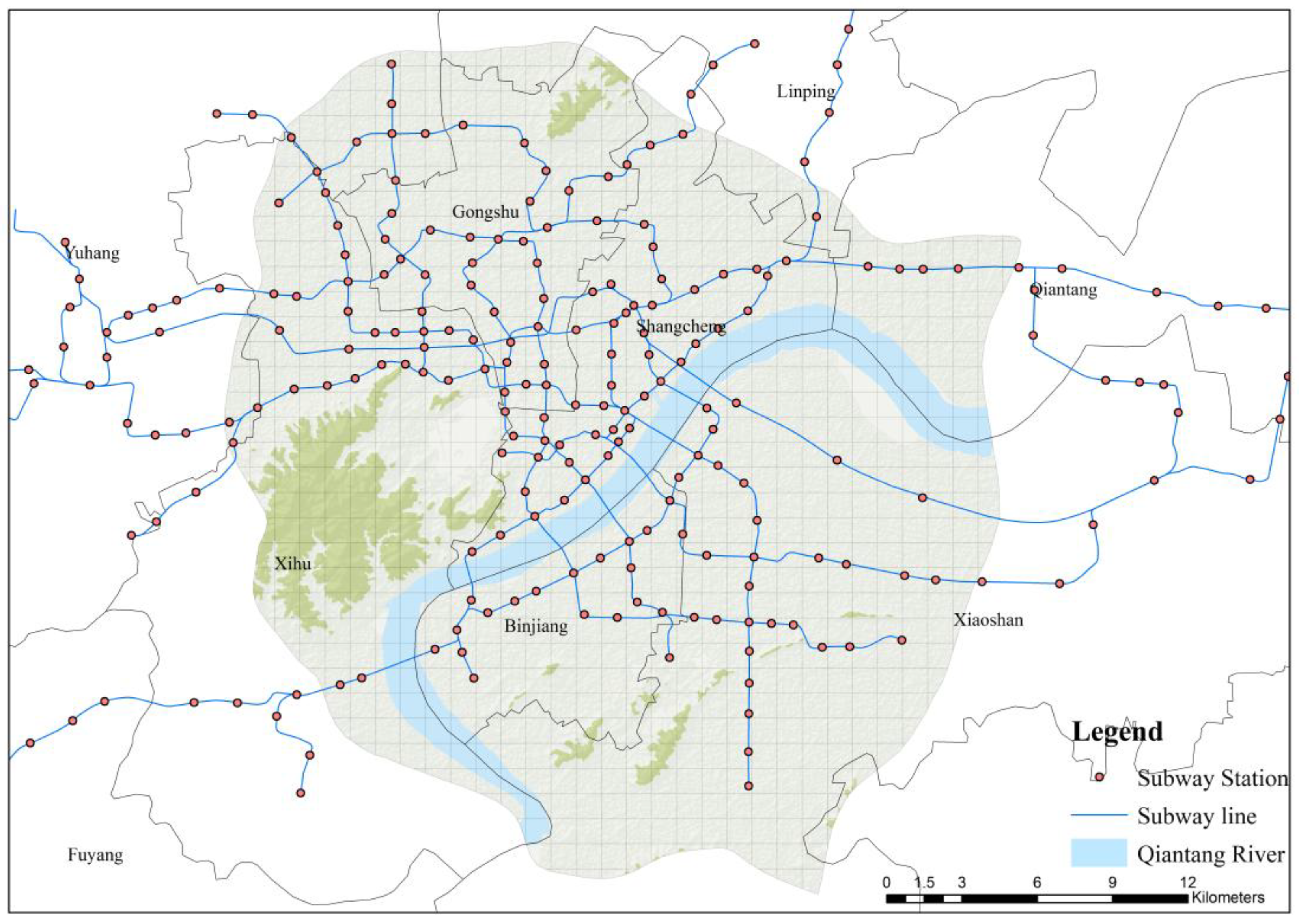
This study uses Hangzhou as the case city. Hangzhou is a prefecture-level city under provincial jurisdiction in China and is the capital of Zhejiang Province. As of 2023, Hangzhou governs ten districts, two counties, and administrates one county-level city. Hangzhou’s urban area includes the old city (Shangcheng District and Gongshu District), the new city (Binjiang District and Qianjiang New City), and functional zones (Xiaoshan District, Yuhang District, and Linping District), with a total area of 16,850 square kilometers (as shown in Figure 4). By the end of 2023, the permanent resident population of Hangzhou was 12.522 million, with an urbanization rate of 84.2%. In terms of public transportation in Hangzhou, Hangzhou Public Transport, as the urban public transportation system serving Hangzhou, Zhejiang Province, China, has a development history of over 100 years. The system covers various modes of transportation, including buses, taxis, water buses, and public bicycles, and has become one of the main choices for Hangzhou residents’ daily travel. In terms of bus services, by the end of December 2022, Hangzhou had as many as 1175 bus routes, 10,217 bus operating vehicles, and a total of 5237 service points (excluding the three counties/cities under Hangzhou’s jurisdiction), and bus travel supports both the National Transportation Union Card and the Hangzhou Tong Bus Card. The bus and metro systems in Hangzhou are indeed managed by two different companies. The bus services are operated by the Hangzhou Public Transport Group, while the metro network is operated by Hangzhou Metro. The key to our analysis is that both systems are part of a city-wide unified smart card (IC card) payment system. This means that residents use the same transit card to pay for trips on both the bus and the metro. In terms of urban rail transit, since the opening of Hangzhou Metro Line 1 in 2012, Hangzhou’s urban rail transit has developed rapidly. By September 2022, apart from 2 suburban lines, there were a total of 12 metro lines in operation in Hangzhou, with a total operating length of approximately 516 km, and 260 metro stations in total, of which 46 are transfer stations.
The research data of this paper were selected from a continuous week of IC card swiping data in Hangzhou from 1 November to 7 November 2023. The original data obtained include a total of six travel information items—card number, departure start time, departure station, arrival station, travel chain end time, and travel record ID—where the travel record ID is an important basis for identifying individual trips in this study. Each record_ID corresponds to a unique travel record, representing a single trip leg (e.g., one bus ride or one metro journey). It was used during the initial data cleaning and validation phase to ensure the integrity of each record. The original desensitized metro card data of Hangzhou are shown in Table 2.
Since the bus smart card data only record the boarding stop and time, the alighting stop and time were inferred using the validated two-stage algorithm proposed by Gao et al. [46]. This step is crucial for obtaining complete OD data for bus trips, which was necessary for constructing the travel chains. Then the original desensitized bus card data were obtained, as shown in Table 3.

4.2. Activity Space Analysis

This study will use ArcGIS software (version 10.8) and Python (version 3.10) to construct the multimodal transportation activity space of residents within Hangzhou’s Ring Expressway. The specific processing method is as follows:
First, the multimodal transportation chain is identified using the bus and metro IC card data and the travel chain identification method in Section 3.1. A total of 453,863 B-R/R-B travel chain data were obtained, including 209,225 B-R travel chain data and 244,638 R-B travel chain data. Second, the travel chain data within Hangzhou’s Ring Expressway are imported into ArcGIS based on the origin locations, then spatially linked with the created Ring Expressway grid data to obtain which travel chain data belong to each grid area. To ensure the reliability of the variance and covariance for constructing the confidence ellipse in subsequent steps, grid areas with fewer than 10 travel chain data points are eliminated after calculation, resulting in travel chains that can be used to calculate the various values of the confidence ellipse (as shown in Table 4).
In the table, ID represents the name of the corresponding grid area; for example, travel chain data with ID n indicates that the travel chain belongs to the n-th grid area. Then, using the above method, the confidence ellipse is drawn. Since there are many grid areas, for the constructed ellipses, we randomly select the data with ID 6 to display the effect, as shown in Figure 5.
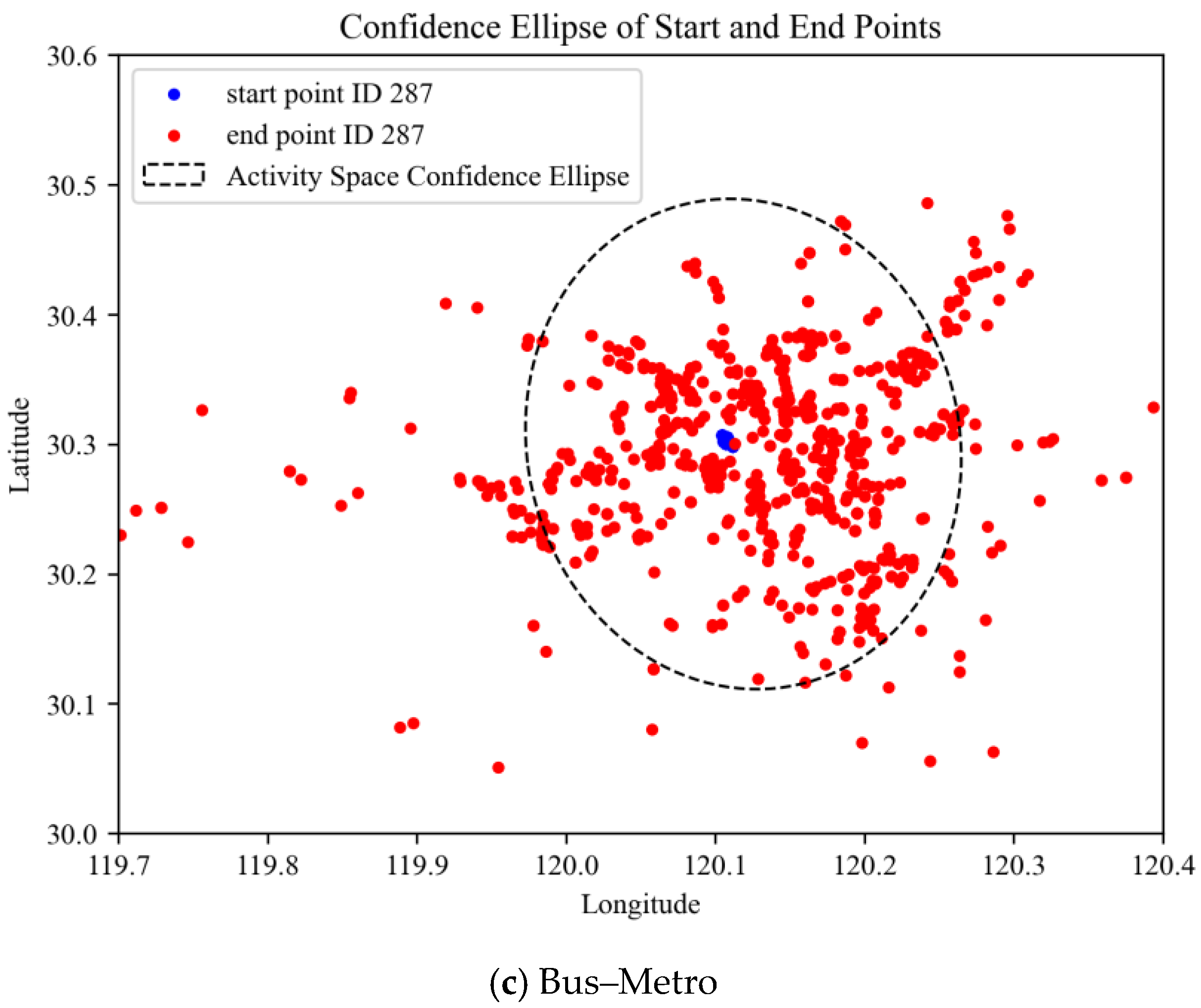
Based on the activity space measurement method in Section 3.2, we calculated and visualized the size of the activity space for grid no. 287 with three different travel modes, as shown in Figure 6. While it is intuitive that combining transport modes would expand an individual’s potential travel range, Figure 6 provides the crucial empirical quantification and visualization of this phenomenon using real-world travel data for a representative grid. It demonstrates that our confidence ellipse method effectively captures the spatial expansion of activity space enabled by multimodal travel. This visual confirmation serves as a vital foundation for the subsequent, more complex modeling analysis, validating the activity space area as a meaningful dependent variable. Figure 6a represents the activity space for pure bus travel, Figure 6b represents the activity space for pure metro travel, and Figure 6c represents the multimodal transportation activity space. It can be seen from the figures that the multimodal transportation activity space is significantly larger than that for pure bus or pure metro travel. This is because the combination of metro and bus can cover a wider area, providing more travel options, thereby expanding people’s activity range. Multimodal-transportation-combined travel can effectively expand people’s activity space and enhance travel experience.
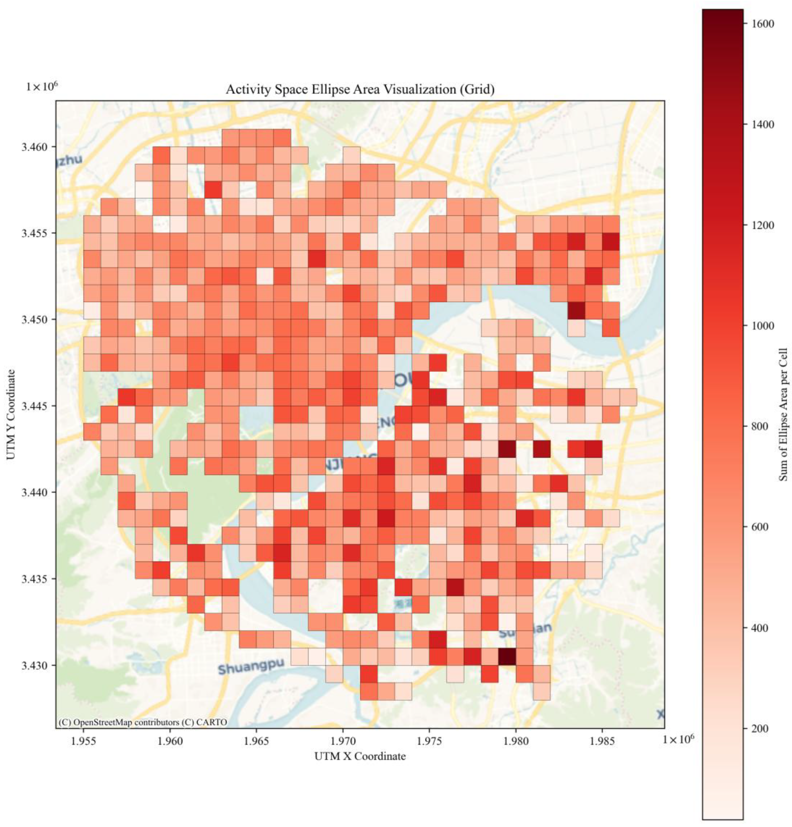
At the same time, we also visualized the size and distribution of the activity space of residents using combined metro–bus multimodal travel, as shown in Figure 7. Residents living in areas closer to the center of Hangzhou have relatively small activity spaces, showing a compact and concentrated pattern; whereas residents farther away from the city center exhibit a more extensive activity space, with their living radius unconsciously expanded.
From the overall planning of Hangzhou, the city center area has numerous commercial shopping centers, educational resources, medical institutions, and other essential facilities. The dense distribution of these facilities greatly meets the daily needs of residents, enabling them to easily access various services without having to travel far. Therefore, residents in the city center naturally have relatively small activity spaces, mostly limited to areas near their residences. In contrast, residents living far from the city center face different living scenarios. Due to the relative scarcity of surrounding facilities, they need to travel longer distances to the city center or other areas to meet specific needs such as shopping, medical treatment, or education. This increased travel demand undoubtedly expands their activity space, resulting in their life trajectories exhibiting a more extensive distribution pattern.

4.3. Variables

4.3.1. Dependent Variable

This study divides Hangzhou’s Ring Expressway area into 1 km × 1 km grids to analyze the influencing factors of the activity space of multimodal transportation for combined bus–metro travel. We select the travel chains (B-R/R-B) for bus–metro transfer trips reaching the destination to construct the activity space for combined bus–metro travel. The dependent variable is the area of the multimodal transportation activity space. For each 1 km × 1 km origin grid (show in Figure 8), we construct a 95% confidence ellipse around the destinations of all multimodal trips starting from that grid. The area of this ellipse is the dependent variable.

4.3.2. Independent Variable

The built environment refers to the external urban geospatial environment provided for human activity needs through human design, modification, and construction, including buildings, infrastructure, public spaces, other artificial environments, transportation networks, parks, commerce areas, and various functional zones that collectively form an interactive geospatial environment. The “3D” elements, originally proposed by [47], include density, diversity, and design. The following is a detailed review of the characteristics of the “3D” elements.
(1)
Density
The “density” indicator measures the level of aggregation of residents, job opportunities, and various activities in different areas of a city. Density indicators are usually measured by residential population density, employment density, and the density of different land use types. This paper uses the density of different land use types to quantify the density characteristics of the city. In this study, Point of Interest (POI) data are used as a high-resolution proxy to represent the density dimension of the built environment, while the diversity dimension is captured through a land use mix index derived from the categorical distribution of POIs [5]. The POI data used in this study was sourced from Gaode Map, one of the most widely used digital mapping service providers in China. The dataset reflects the spatial distribution of POIs in 2023 and was subjected to standard preprocessing procedures, including the removal of duplicates, geocoding verification, and spatial filtering within the study area. POI categories were defined based on Gaode’s classification system. Specifically, commercial POIs include shopping malls, department stores, supermarkets, and convenience stores; catering POIs include restaurants, cafes, snack bars, and pubs; science and education POIs include universities, schools, kindergartens, libraries, and museums; residential POIs include apartment buildings, housing estates, and residential communities, and healthcare POI include hospitals, clinics, and community health centers.
(2)
Diversity
The mixing degree is also known as diversity. This indicator assesses the degree of mixing of different types of land cover/land use within a specific research scale. In previous studies of the built environment, researchers often used land use mix to measure the diversity of an area. A lower value of mixing degree usually indicates that the land use types in the area are relatively homogeneous, with a low degree of mixing. Conversely, if an area has a higher mixing degree, it means that the land use types are more diverse and the degree of mixing is higher. By adjusting the mixing degree of land types, residents can achieve multiple travel purposes in high mixing degree areas. This can effectively reduce the time required for commuting.
(3)
Design
Urban design research focuses on the layout characteristics of internal roads and municipal facilities and their impact on the built environment. This paper provides quantitative support for analyzing the geospatial interaction mechanism between urban design elements and the built environment by integrating three dimensions: road systems, the accessibility of public transportation facilities, and geospatial location. Therefore, this paper selects road network density, distance to the city center, the number of bus stops in each grid, the number of metro stations within 3 km, and the distance to the nearest metro station as criteria for evaluating built environment design elements.
According to the literature review, in addition to considering built environment factors, socioeconomic characteristics are also essential independent variables. This paper uses the 1 km historical GDP geospatial distribution grid dataset of mainland China, selecting Hangzhou’s 2023 GDP data to reflect the economic status of each grid.
Before building the model, in order to address potential multicollinearity among the variables, this study eliminated the variables highly correlated with others by calculating the Variance Inflation Factor (VIF); road density was excluded because its VIF was greater than 7.5, and ultimately all variables used for modeling had VIF values less than 7.5, indicating that there was no severe multicollinearity. The statistical data for the dependent and independent variables used for modeling are shown in Table 5.

5. Results and Analysis

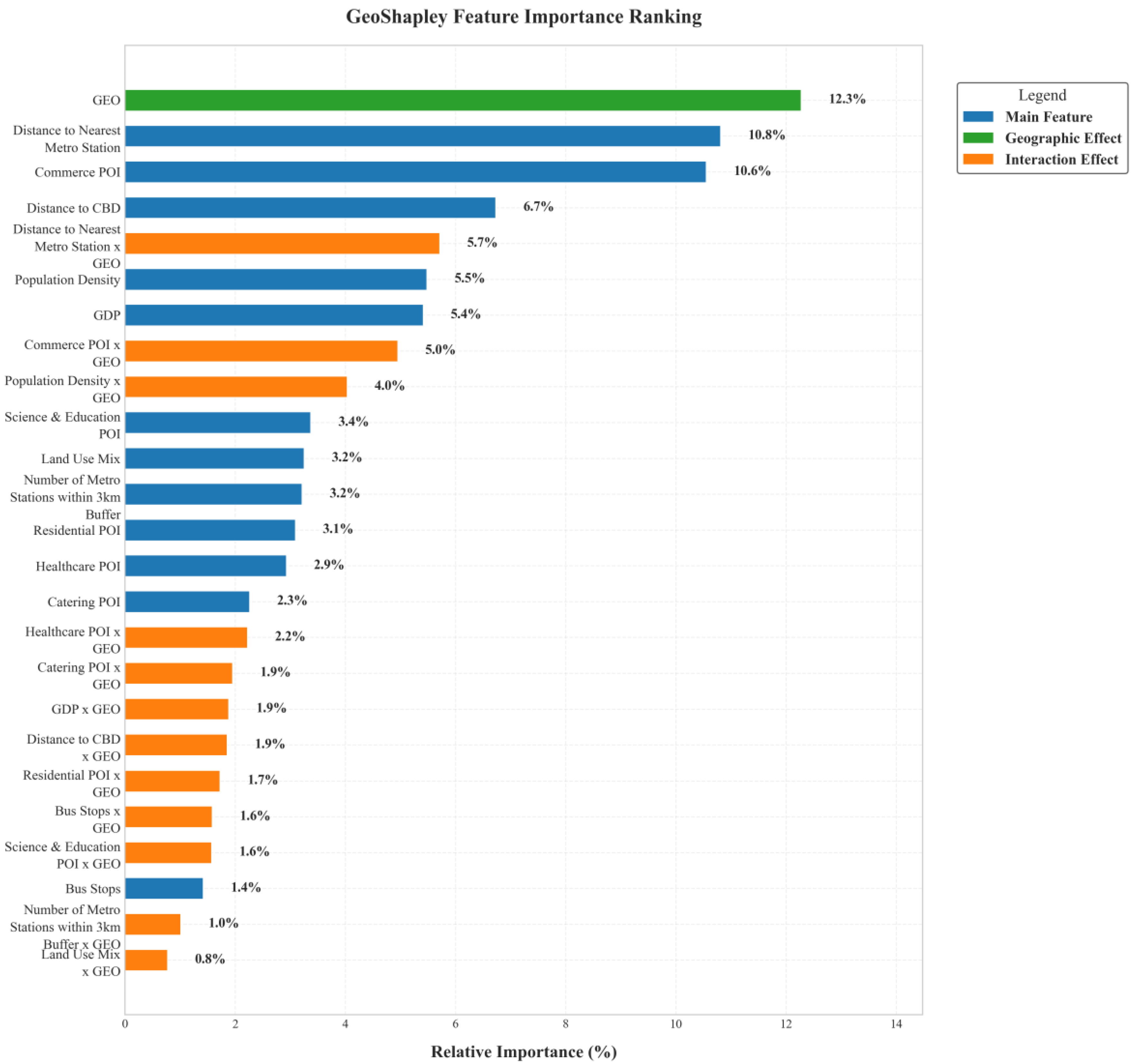
In this section, we will use the variables, which have passed the multicollinearity test, to build an XGBoost model to explore the influencing factors of multimodal transportation activity space. It should be noted that overfitting and underfitting are issues that must be addressed when training nonlinear models. Selecting appropriate hyperparameters can effectively prevent the XGBoost model from overfitting or underfitting. The learning rate, the maximum number of regression trees, and the maximum depth are important controllable factors affecting the model’s fitting ability. This paper uses Bayesian hyperparameter tuning to optimize the hyperparameters of the XGBoost model in order to choose the best parameter combination. After parameter tuning, the model for combined metro–bus travel is set with a tree depth of 3, a learning rate of 0.01, and a maximum number of 337 regression trees. The variables are incorporated into the XGBoost model to explore the influencing factors of multimodal transportation activity space. The modeling results are shown in Table 6.

5.1. Relative Importance of Explanatory Variables

Figure 9 reveals the relative importance of the influencing factors of multimodal transportation activity space through GeoShapley. In the model, GEO, the distance to the nearest metro station, and the number of commercial POIs rank in the top three in importance. Here, “GEO” represents the total contribution of the location features. This indicates that geographic factors and the design elements in the built environment are key factors affecting the area of the multimodal activity space. Geographic factors have a very important impact on the activity space of multimodal transportation users, and many interaction variables between independent variables and GEO also have significant influences. The features labeled with ‘x GEO’ represent the interaction effects calculated by the GeoShapley method, not new input variables. An interaction effect measures how the importance of a main feature is modified by geographic location.

5.2. Nonlinear Relationship Analysis of Key Variables

In this section, we select four representative variables with relatively high feature importance in the model for separate analysis; to visualize these nonlinear effects, we use partial dependence plots (PDPs). A PDP isolates the marginal effect of one feature on the model’s prediction while averaging out the effects of all other features.
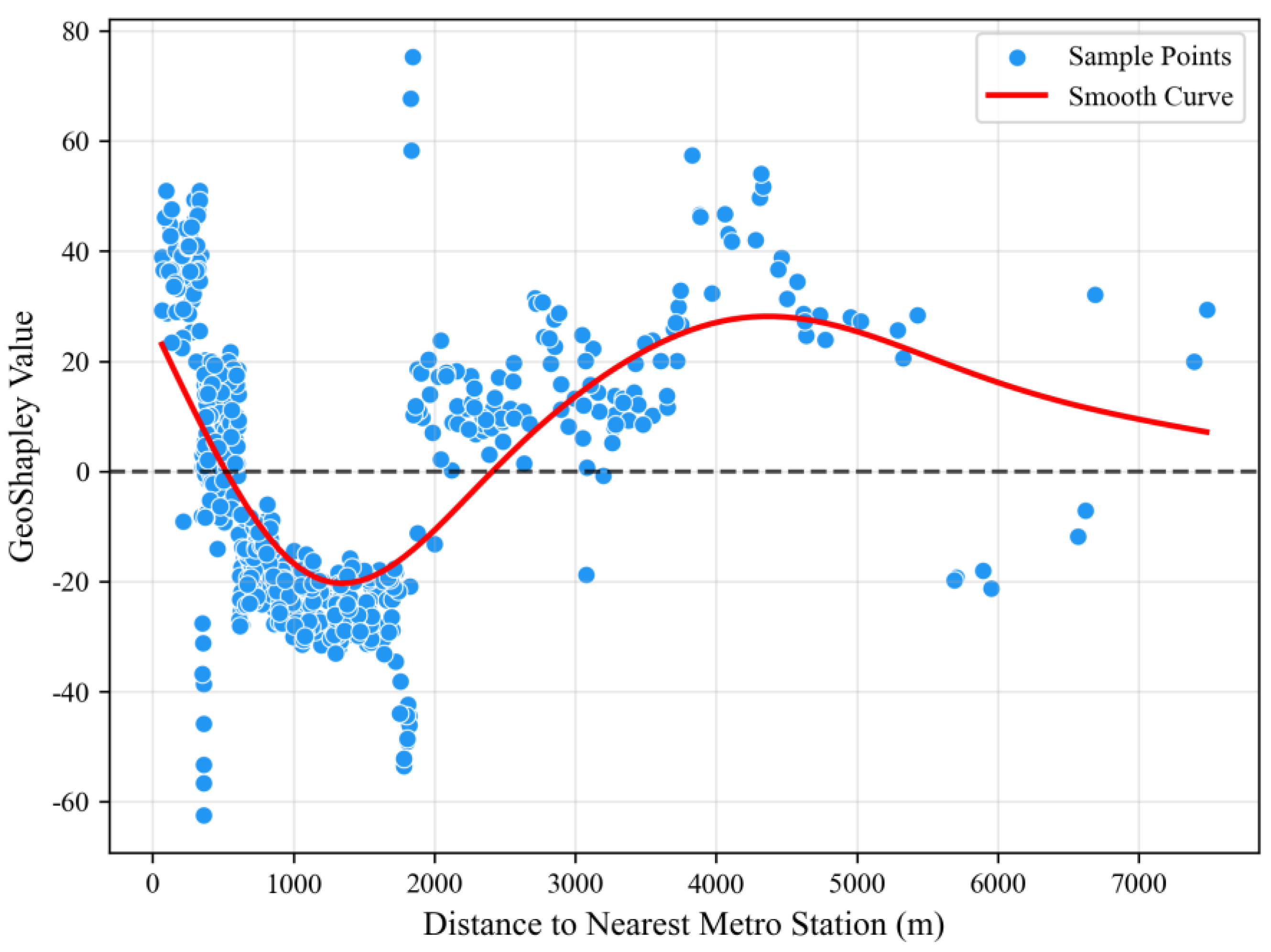
Figure 10 shows the relationship between the area of residents’ multimodal transportation activity space and the distance to the nearest metro station. It can be seen from the figure that as the distance to the nearest metro station increases, the GeoShapley value exhibits a nonlinear trend. Within a relatively close distance to the nearest metro station (approximately 0–1000 m), the GeoShapley value drops rapidly. This might be because the area close to the metro station offers more convenient living conditions and a relatively smaller activity range, or residents can reach their destinations directly by metro without the need for bus connections. Between 1000 m and 7000 m from the nearest metro station, the GeoShapley value shows a fluctuating upward trend, followed by a slight decline. This indicates that as the distance increases, the area of residents’ activity space gradually enlarges, possibly because areas far from the metro station have inconvenient transportation, and residents need to use buses to connect to the metro, thereby creating a larger activity space to meet daily or commuting needs. Overall, the relationship between the area of residents’ multimodal transportation activity space and the distance to the nearest metro station exhibits nonlinear characteristics, reflecting changes in travel modes and activity ranges within different distance ranges.
Figure 11 shows the impact of the distance to the CBD on the multimodal transportation activity space of residents. In the model, in areas closer to the CBD (0–10,000 m), the GeoShapley value is relatively small, possibly because these areas are convenient for living, and residents’ activity spaces are relatively concentrated [48]. Then, as the distance further increases, the GeoShapley value begins to rise rapidly. Areas far from the CBD cannot adequately meet people’s living and commuting needs, so residents require a broader activity space to meet their daily commuting and living requirements. This indicates that residents farther from the CBD are more inclined to use combined metro–bus travel to reach their destinations because the advantages in speed and cost-effectiveness can reduce the travel time for suburban residents.
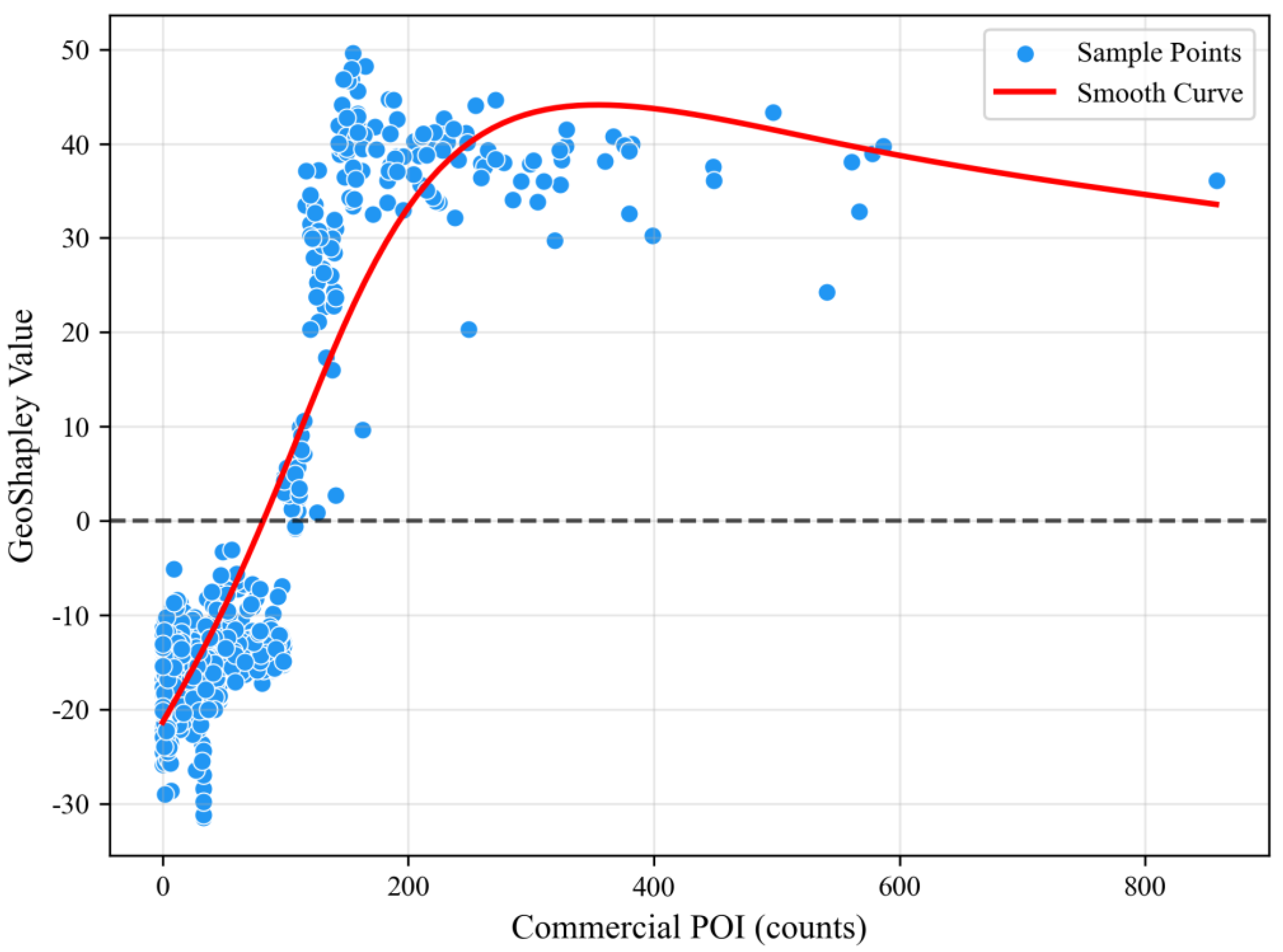
Figure 12 shows the relationship between the residents, multimodal transportation activity space, and the number of commercial POIs. It can be seen from the figure that as the number of commercial POIs increases, the GeoShapley value also shows a certain trend. Specifically, when the number of commercial POIs is relatively small (approximately 0–100), the GeoShapley value fluctuates greatly and shows an overall upward trend. When the number of commercial POIs reaches a certain value (approximately 100–200), the increase in GeoShapley value tends to level off and remains stable to some extent. With a further increase in the number of commercial POIs (exceeding 200), the variation in the GeoShapley value diminishes, even slightly decreasing. This phenomenon may be due to the agglomeration effects of commercial facilities, an economic principle in which the spatial clustering of businesses and services generates synergistic benefits—such as a larger customer base and shared infrastructure—that in turn attract greater levels of human activity and mobility to the area. When the number of commercial POIs is low, as the number increases, commercial facilities gradually improve, attracting more people and activities, thereby increasing residents’ activity space. But when the number of commercial POIs reaches a certain scale, the impact of commercial facilities on residents’ activity space becomes saturated.
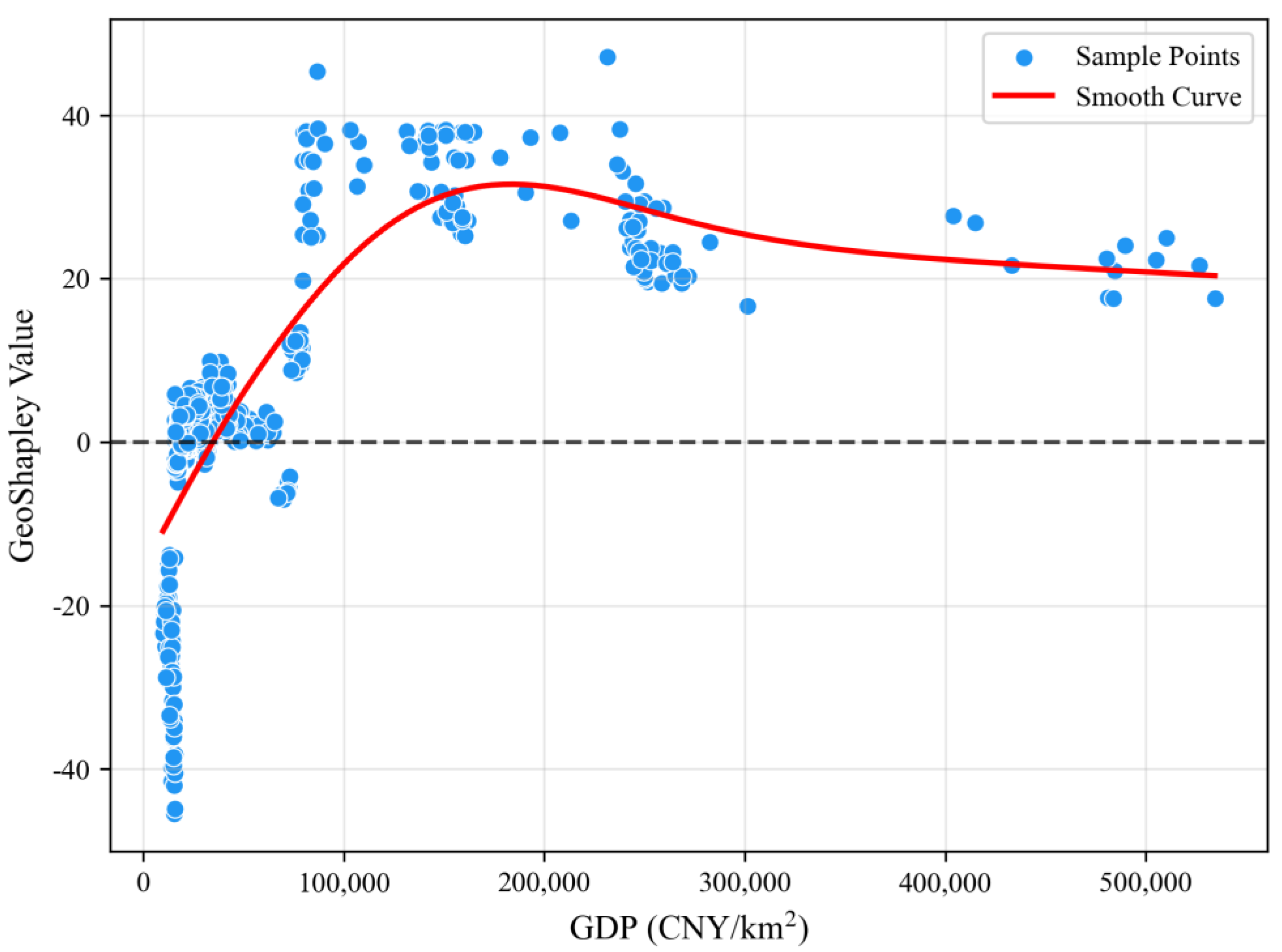
Figure 13 shows the impact of GDP on the multimodal transportation activity space of residents. In the model, as GDP increases, the GeoShapley value first increases and then tends to stabilize or even slightly decrease. At low GDP levels, residents’ activity space is relatively small; as GDP increases, the area of activity space increases significantly. When GDP reaches a certain level, the growth trend of the activity space slows down and eventually slightly decreases. This may be because GDP is an important indicator of economic development; as GDP increases, residents’ income levels rise and they have more resources for travel and activities, leading to an increase in the area of activity space. However, after GDP reaches a certain level, residents have more travel options and may no longer pursue the cost-effectiveness of combined metro–bus travel, possibly switching to cars, ride-hailing, or other more convenient and faster travel modes.

5.3. Geospatial Effect Analysis

The greatest advantage of GeoShapley over traditional SHAP interpretability models is that it can perform geospatial effect analysis and display the results on a map. Next, this paper will analyze the impact of geographic location on activity space as well as the impact of the interaction effects between geographic location and two important independent variables on activity space. The values of the legends in the figures are still GeoShapley values, which are mentioned in the GeoShapley section.
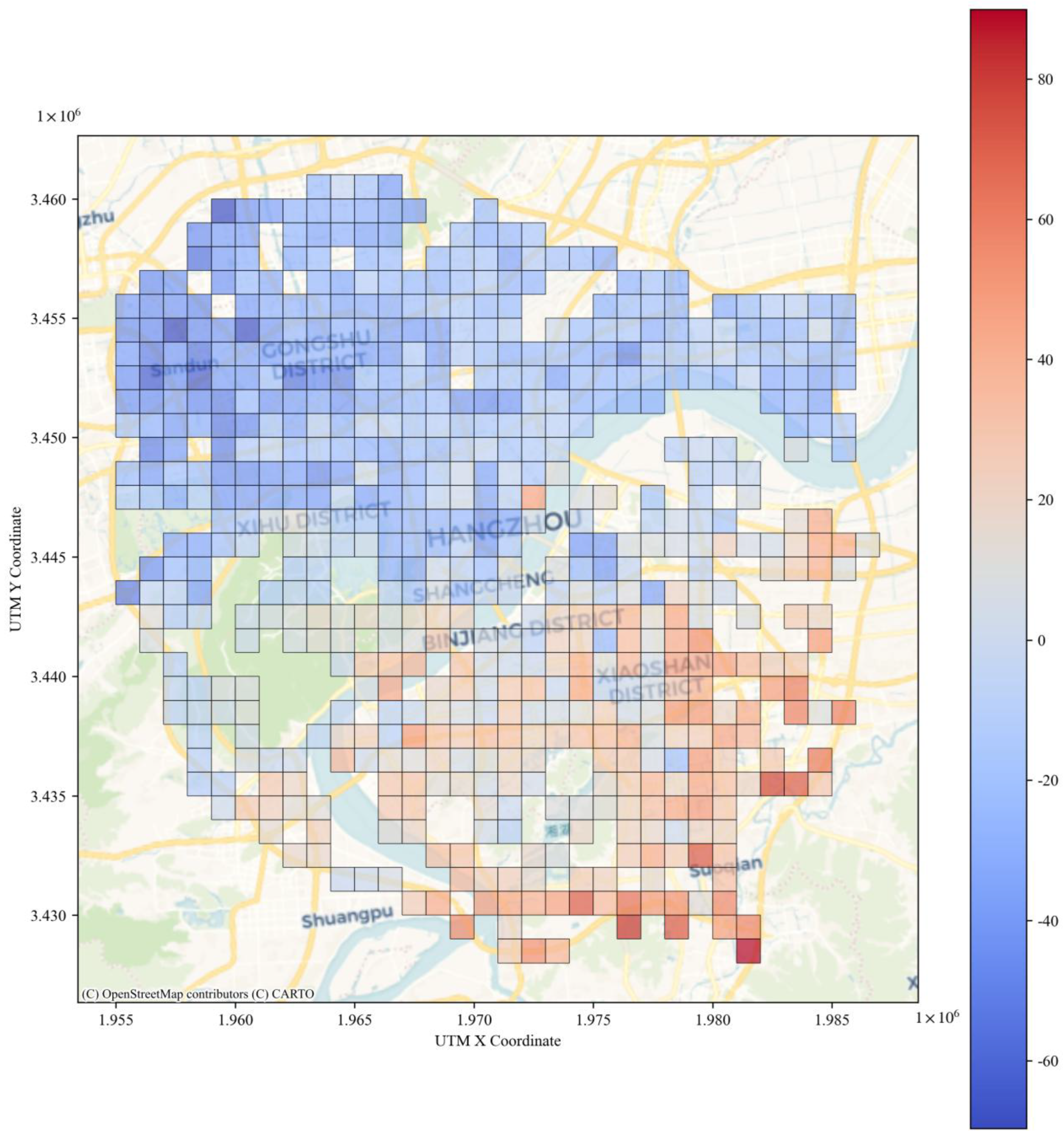
Figure 14 is a geospatial effect figure showing the impact of GEO on the multimodal transportation activity space of residents. The model indicates that areas on the south side of the Qiantang River have a greater impact on residents’ activity space than those on the north side. It can be seen that public transportation resources in areas on the south side of the Qiantang River are relatively scarce, and combined metro–bus travel brings very positive effects to residents in the Xiaoshan District and Hangzhou South Station area; the further south, the larger the activity space for combined metro–bus travel. The color scale represents the GeoShapley value. Positive values (in red) indicate that the geographic location (or its interaction with a feature) contributes to a larger-than-average activity space, while negative (in blue) values indicate a contribution to a smaller-than-average activity space.
Figure 15 is a geospatial effect figure showing the interaction between GEO and the variable “distance to the nearest metro station” on residents’ multimodal transportation activity space, showing the strength of the correlation between the distance from a specific location to the nearest metro station and the size of residents’ multimodal transportation activity space. It can be seen that in the areas around Xihu District, Binjiang District, and near Hangzhou’s city center, the distance to the nearest metro station is weakly correlated with residents’ activity space, while in other regions the correlation is stronger. This indicates that, except for the areas mentioned above, when the distance to the nearest metro station decreases (for example, through the construction of new metro stations), residents’ multimodal transportation activity space will also decrease, proving that these areas still have sufficient transportation potential and a certain gap in transportation resources, so if new metro stations can facilitate people’s travel, the activity space can be reduced to some extent.

6. Conclusions and Policy Implication

This study, through the measurement and analysis of the multimodal transportation activity space in Hangzhou, reveals the interrelationships among different travel modes in the urban transportation system and their impact on residents’ travel activity space. The results emphasize the necessity of incorporating multimodal perspectives into urban transportation planning to enhance system-wide efficiency, equity, and sustainability. The main conclusions are as follows:
(1)
By integrating bus and metro smart card data, we extract detailed multimodal travel chains that record residents’ origins, destinations, travel durations, and transport modes. A total of 453,863 B-R/R-B travel chain data points were obtained, including 209,225 B-R travel chain data points and 244,638 R-B travel chain data points. These chains offer a comprehensive view of urban public transit use across multiple modes.
(2)
Using grid-based analysis and confidence ellipses, we measured the spatial extent of activity spaces under different travel modes. Compared with single-mode travel (bus-only or metro-only), multimodal travel significantly enlarges residents’ activity spaces, demonstrating the spatial complementarity between transport modes.
(3)
The research results indicate that the characteristics of multimodal transportation activity space are influenced not only by transportation infrastructure but are also closely related to urban environmental characteristics and socioeconomic features. Specifically, factors such as the distance to the nearest metro station, the distance to the CBD, the distribution of commercial facilities, and GDP exhibit significant nonlinear characteristics in their influence on the activity space of multimodal transportation residents, and the interaction between the distance to the nearest metro station and geographic location also produces strong spatial effects. Through the combination of the XGBoost and GeoShapley models, we can deeply understand the key factors influencing multimodal transportation activity space and their spatial interactions.
Based on the above conclusions, the following policy implications can be provided:
(1)
Optimize transportation infrastructure layout and enhance service coverage. This policy is supported by the geospatial interaction analysis in Figure 15. The analysis reveals that in central areas such as Xihu District, Binjiang District, and downtown Hangzhou, the distance to the nearest metro station shows a weak correlation with residents’ activity spaces. In contrast, this correlation is much stronger in peripheral areas, indicating an unmet demand for public transit. These findings suggest that expanding public transportation infrastructure in under-served regions could significantly enhance residents’ mobility and unlock latent travel potential, thereby improving spatial equity in the access to urban opportunities [6,49].
(2)
Enhance mobility support for low-income populations. The recommendation to enhance mobility support for low-income populations is directly informed by the nonlinear relationship shown in Figure 13. The study finds that the multimodal transportation activity space of low-income groups is relatively limited [34]. It is therefore recommended that transportation policies incorporate targeted subsidies and service improvements for low-income areas [50]. In future research, it would also be valuable to examine the integration of public transportation with green travel modes, such as cycling, to explore how more diversified and sustainable travel options could benefit low-income populations. These directions may contribute to improving mobility equity while supporting the broader goals of sustainable urban development and social inclusion.
(3)
Implement differentiated strategies to expand residents’ activity spaces. The recommendation to implement differentiated strategies for commercial facility planning is grounded in the threshold effect observed in Figure 12. Priority should be given to planning small, convenient commercial facilities (such as convenience stores and community markets) in areas with a lower density of commercial POIs (e.g., communities with POI numbers < 200), thereby stimulating the potential for residents’ activity space by enhancing basic commercial accessibility; whereas in areas where POIs are saturated (e.g., POI > 200), the focus should shift to optimizing the commercial format and spatial distribution (such as reducing homogeneous shops and increasing open spaces like community plazas). Low-density areas should focus on “incremental quality improvement”, and high-density areas on “stock optimization”. This is in line with the “diseconomies of agglomeration” theory in new economic geography research [51] and the principle of supply–demand balance in public spaces, thereby avoiding diminishing marginal returns due to over-agglomeration, and achieving the efficient expansion of residents’ activity space through differentiated strategies.
(4)
Our findings offer tangible tools for planners. The geospatial effect maps (Figure 14 and Figure 15) can be used as a diagnostic tool to identify ‘transportation potential area’ where the distance to a metro station strongly and negatively impacts residents’ mobility. These areas, particularly in the urban periphery, should be prioritized for investment in feeder bus services or new transit infrastructure.

Limitation

Although this study offers valuable insights into the measurement and influencing mechanisms of multimodal transportation activity spaces, several limitations should be acknowledged. Firstly, due to data constraints, the analysis is limited to two public transit modes—bus and metro. It excludes other travel modes such as walking, cycling, private cars, and ride-hailing, which are essential components of an integrated urban transport system. Future research should strive to integrate data from multiple sources (e.g., GPS tracking, travel diaries, bike-sharing systems) to construct a more holistic picture of true multimodal activity spaces. Secondly, the data covers only a specific time period and does not reflect seasonal, holiday, or event-driven variations, potentially limiting the understanding of temporal dynamics in activity space. Thirdly, although various built environment and socioeconomic factors are considered, the complex interactions among them may not be fully captured. Future research could address these limitations by incorporating a wider range of travel modes and using longitudinal data to better reflect spatiotemporal dynamics. In addition, combining big data with individual-level survey data would help account for user-specific attributes (e.g., age, gender, occupation), allowing for a more nuanced analysis of behavioral heterogeneity and contextual factors shaping multimodal mobility.
Finally, while our models reveal complex nonlinear associations, they do not establish causality. The underlying behavioral mechanisms driving residents’ travel decisions—such as personal preferences, trip purpose, and real-time constraints—are not captured. Future research could integrate qualitative methods, such as surveys or interviews, to explore the ‘why’ behind the observed spatial patterns and strengthen the explanatory power of the findings.

Author Contributions

Conceptualization, Kuang Guo, Haixiao Pan and Yang Liu; methodology, Haixiao Pan and Zhuangbin Shi; software, Rui Tang, Zhuangbin Shi and Dongming Zhang; formal analysis, Rui Tang and Dongming Zhang; resources, Kuang Guo; data curation, Kuang Guo and Haixiao Pan; writing—original draft preparation, Kuang Guo, Rui Tang, Yang Liu and Haixiao Pan; writing—review and editing, Kuang Guo and Haixiao Pan; visualization, Rui Tang, Zhuangbin Shi and Dongming Zhang; supervision, Kuang Guo; funding acquisition, Yang Liu and Zhuangbin Shi. All authors have read and agreed to the published version of the manuscript.

Funding

This research was funded by the National Natural Science Foundation of China (Grant No. 52202381), Yunnan Fundamental Research Projects (Grant Nos. 202401AT070373, 202201BE070001-052), and Yunnan Xing Dian Talents Plan Young Program (KKRD202202110, 2022).

Data Availability Statement

The data are not publicly available due to privacy or ethical restrictions.

Acknowledgments

Thanks to the school, the research platform, and the research partners who participated in the discussion. In the process of completing this paper, everyone gave us selfless help and advice, and we sincerely thank everyone who helped us in our research.

Conflicts of Interest

On behalf of all authors, the corresponding author states that there are no known competing financial interests or personal relationships that could have appeared to influence the work reported in this paper.

Appendix A

Here are the details of the XGBoost model:
Model representation: XGBoost constructs an ensemble of decision trees to make predictions. For a given dataset x i , y i , where x i represents the features and y i the target values, the prediction function of XGBoost is expressed as follows:
y i = t = 1 T   f t x i
Here, f t denotes the t -th decision tree, and T is the total number of trees in the model.
Loss function and regularization: The optimization of XGBoost is driven by a regularized loss function, which balances model fit and complexity. The objective function at the t -th iteration is given by the following:
L ( t ) = i = 1 n   l y i , y i ( t 1 ) + f t x i + Ω f t
The regularization term Ω f t is defined as follows:
Ω ( f ) = γ T + 1 2 λ j = 1 T   w j 2
where γ and λ are regularization parameters, and w j represents the weights of the leaf nodes. This regularization helps prevent overfitting by penalizing complex models.
Gradient boosting mechanism: XGBoost employs a second-order Taylor expansion to approximate the loss function, facilitating efficient gradient boosting as follows:
L ( t ) i = 1 n   g i f t x i + 1 2 h i f t x i 2 + Ω f t
where g i and h i are the first and second derivatives of the loss function, respectively, and calculated as follows:
g i = / y i , y i ( t 1 ) y i ( t 1 )
h i = 2 / y i , y i ( t 1 ) y i ( t 1 ) 2
Tree construction and optimization: Each decision tree in XGBoost is constructed using a greedy algorithm that selects split points to maximize the gain as follows:
  Gain = 1 2 G L 2 H L + λ + G R 2 H R + λ G L + G R 2 H L + H R + λ γ
where G L and G R are the sums of the first derivatives for the left and right branches, and H L and H R are the sums of the second derivatives.
In summary, XGBoost’s robust framework, characterized by its regularized objective function and efficient gradient boosting mechanism, makes it a powerful tool for predictive modeling. Its ability to handle diverse data types and its scalability have established it as a preferred choice in both academic research and practical applications.

References

  1. Makarova, I.; Shubenkova, K.; Pashkevich, A. Efficiency Assessment of Measures to Increase Sustainability of the Transport System. Transport 2021, 36, 123–133. [Google Scholar] [CrossRef]
  2. Hasanzadeh, K.; Kyttä, M.; Lilius, J.; Ramezani, S.; Rinne, T. Centricity and multi-locality of activity spaces: The varying ways young and old adults use neighborhoods and extra-neighborhood spaces in Helsinki Metropolitan Area. Cities 2021, 110, 103062. [Google Scholar] [CrossRef]
  3. Cagney, K.A.; York Cornwell, E.; Goldman, A.W.; Cai, L. Urban Mobility and Activity Space. Annu. Rev. Sociol. 2020, 46, 623–648. [Google Scholar] [CrossRef]
  4. Zheng, N.; Geroliminis, N. On the Distribution of Urban Road Space for Multimodal Congested Networks. Procedia-Soc. Behav. Sci. 2013, 80, 119–138. [Google Scholar] [CrossRef]
  5. Gong, L.; Jin, M.; Liu, Q.; Gong, Y.; Liu, Y. Identifying Urban Residents’ Activity Space at Multiple Geographic Scales Using Mobile Phone Data. ISPRS Int. Geo-Inf. 2020, 9, 241. [Google Scholar] [CrossRef]
  6. Gao, Q.-L.; Yue, Y.; Zhong, C.; Cao, J.; Tu, W.; Li, Q.-Q. Revealing transport inequality from an activity space perspective: A study based on human mobility data. Cities 2022, 131, 104036. [Google Scholar] [CrossRef]
  7. Litman, T. Toward More Comprehensive and Multi-Modal Transport Evaluation; Citeseer: University Park, PA, USA, 2013. [Google Scholar]
  8. Liu, Y.; Ji, Y.; Feng, T.; Timmermans, H. Understanding the determinants of young commuters’ metro-bikeshare usage frequency using big data. Travel Behav. Soc. 2020, 21, 121–130. [Google Scholar] [CrossRef]
  9. Fu, X.; Lam, W.H.; Meng, Q. Modelling impacts of adverse weather conditions on activity–travel pattern scheduling in multi-modal transit networks. Transp. B Transp. Dyn. 2014, 2, 151–167. [Google Scholar] [CrossRef]
  10. Du, M.; Li, X.; Kwan, M.-P.; Yang, J.; Liu, Q. Understanding the Spatiotemporal Variation of High-Efficiency Ride-Hailing Orders: A Case Study of Haikou, China. ISPRS Int. Geo-Inf. 2022, 11, 42. [Google Scholar] [CrossRef]
  11. Li, Q.; Cui, C.; Liu, F.; Wu, Q.; Run, Y.; Han, Z. Multidimensional Urban Vitality on Streets: Spatial Patterns and Influence Factor Identification Using Multisource Urban Data. ISPRS Int. Geo-Inf. 2022, 11, 2. [Google Scholar] [CrossRef]
  12. Deng, X.; Jiang, S. An Overview about Research on 3D Visualization Technology of Geographic Information Based on Computer Software Development. J. Phys. Conf. Ser. 2020, 1648, 032124. [Google Scholar] [CrossRef]
  13. Chai Yan-Wei, S.J. Activity-based Approach to Human Spatial Behavior Research. Sci. Geogr. Sin. 2008, 28, 594–600. [Google Scholar] [CrossRef]
  14. Wang, D.; Li, F.; Chai, Y. Activity Spaces and Sociospatial Segregation in Beijing. Urban Geogr. 2012, 33, 256–277. [Google Scholar] [CrossRef]
  15. Na, T.A.; Yanwei, C. Disciplinary position and research frontiers of behavioral geography. Prog. Geogr. 2022, 41, 1–15. [Google Scholar] [CrossRef]
  16. Shen Yue, C.Y. Daily activity space of suburban mega-community residents in Beijing based on GPS data. Acta Geogr. Sin. 2013, 68, 506–516. [Google Scholar] [CrossRef]
  17. Hägerstrand, T. What about people in Regional Science? Pap. Reg. Sci. Assoc. 1970, 24, 6–21. [Google Scholar] [CrossRef]
  18. Miller, H.J. Modelling accessibility using space-time prism concepts within geographical information systems. Int. J. Geogr. Inf. Syst. 1991, 5, 287–301. [Google Scholar] [CrossRef]
  19. Dijst, M. Two-earner families and their action spaces: A case study of two Dutch communities. GeoJournal 1999, 48, 195–206. [Google Scholar] [CrossRef]
  20. Newsome, T.H.; Walcott, W.A.; Smith, P.D. Urban activity spaces: Illustrations and application of a conceptual model for integrating the time and space dimensions. Transportation 1998, 25, 357–377. [Google Scholar] [CrossRef]
  21. Buliung, R.N.; Kanaroglou, P.S. A GIS toolkit for exploring geographies of household activity/travel behavior. J. Transp. Geogr. 2006, 14, 35–51. [Google Scholar] [CrossRef]
  22. Golledge, R.G. Wayfinding Behavior: Cognitive Mapping and Other Spatial Processes; JHU Press: Baltimore, MD, USA, 2010. [Google Scholar]
  23. Schönfelder, S.; Axhausen, K.W. Activity spaces: Measures of social exclusion? Transp. Policy 2003, 10, 273–286. [Google Scholar] [CrossRef]
  24. Zhou, Y.; Fang, Z.; Thill, J.-C.; Li, Q.; Li, Y. Functionally critical locations in an urban transportation network: Identification and space–time analysis using taxi trajectories. Comput. Environ. Urban Syst. 2015, 52, 34–47. [Google Scholar] [CrossRef]
  25. Li, J.; Zheng, P.; Zhang, W. Identifying the spatial distribution of public transportation trips by node and community characteristics. Transp. Plan. Technol. 2020, 43, 325–340. [Google Scholar] [CrossRef]
  26. Wang, L.; Li, X.; Ding, L.; Yu, X.; Hu, T. Visualization and Analysis of Transport Accessibility Changes Based on Time Cartograms. ISPRS Int. Geo-Inf. 2022, 11, 432. [Google Scholar] [CrossRef]
  27. Yu, H.; Shaw, S.L. Exploring potential human activities in physical and virtual spaces: A spatio-temporal GIS approach. Int. J. Geogr. Inf. Sci. 2008, 22, 409–430. [Google Scholar] [CrossRef]
  28. Ding, W.; Yang, X.; Wu, S. A review of activity-based travel behavior research. Hum. Geogr. 2008, 23, 85–91. [Google Scholar] [CrossRef]
  29. Xu, M.; Lam, W.H.; Gao, Z.; Grant-Muller, S. An activity-based approach for optimisation of land use and transportation network development. Transp. B Transp. Dyn. 2016, 4, 111–134. [Google Scholar] [CrossRef]
  30. Duan, Z.; Zhao, H.; Li, Z. Non-linear effects of built environment and socio-demographics on activity space. J. Transp. Geogr. 2023, 111, 103671. [Google Scholar] [CrossRef]
  31. Dharmowijoyo, D.B.E.; Susilo, Y.O.; Karlström, A. Relationships among discretionary activity duration, its travel time spent and activity space indices in the Jakarta Metropolitan Area, Indonesia. J. Transp. Geogr. 2016, 54, 148–160. [Google Scholar] [CrossRef]
  32. Kemperman, A.D.A.M.; Timmermans, H.J.P. Influence of Socio-Demographics and Residential Environment on Leisure Activity Participation. Leis. Sci. 2008, 30, 306–324. [Google Scholar] [CrossRef]
  33. Chen, N.; Akar, G. How do socio-demographics and built environment affect individual accessibility based on activity space? Evidence from Greater Cleveland, Ohio. J. Transp. Land Use 2016, 10, 477–503. [Google Scholar] [CrossRef]
  34. Tao, S.; He, S.Y.; Kwan, M.-P.; Luo, S. Does low income translate into lower mobility? An investigation of activity space in Hong Kong between 2002 and 2011. J. Transp. Geogr. 2020, 82, 102583. [Google Scholar] [CrossRef]
  35. Sharmeen, N.; Houston, D. Spatial Characteristics and Activity Space Pattern Analysis of Dhaka City, Bangladesh. Urban Sci. 2019, 3, 36. [Google Scholar] [CrossRef]
  36. Zheng, J.; Hu, M.; Wang, C.; Wang, S.; Han, B.; Wang, H. Spatial patterns of residents’ daily activity space and its influencing factors based on the CatBoost model: A case study of Nanjing, China. Front. Archit. Res. 2022, 11, 1193–1204. [Google Scholar] [CrossRef]
  37. Chen, N.; Akar, G. Effects of neighborhood types & socio-demographics on activity space. J. Transp. Geogr. 2016, 54, 112–121. [Google Scholar] [CrossRef]
  38. Tana; Kwan, M.-P.; Chai, Y. Urban form, car ownership and activity space in inner suburbs: A comparison between Beijing (China) and Chicago (United States). Urban Stud. 2016, 53, 1784–1802. [Google Scholar] [CrossRef]
  39. Yang, L.; Yang, H.; Yu, B.; Lu, Y.; Cui, J.; Lin, D. Exploring non-linear and synergistic effects of green spaces on active travel using crowdsourced data and interpretable machine learning. Travel Behav. Soc. 2024, 34, 100673. [Google Scholar] [CrossRef]
  40. Liu, D.; Lu, Y.; Yang, L. Exploring non-linear effects of environmental factors on the volume of pedestrians of different ages using street view images and computer vision technology. Travel Behav. Soc. 2024, 36, 100814. [Google Scholar] [CrossRef]
  41. Liu, Y.; He, D.; Lei, J.; He, M.; Shi, Z. Investigating the non-linear influence of the built environment on passengers’ travel distance within metro and bus networks using smart card data. Multimodal Transp. 2025, 4, 100188. [Google Scholar] [CrossRef]
  42. Huang, Z.; Xu, L.; Lin, Y.; Wu, P.; Feng, B. Citywide Metro-to-Bus Transfer Behavior Identification Based on Combined Data from Smart Cards and GPS. Appl. Sci. 2019, 9, 3597. [Google Scholar] [CrossRef]
  43. Liu, C.; Susilo, Y.O.; Dharmowijoyo, D.B.E. Investigating intra-household interactions between individuals’ time and space constraints. J. Transp. Geogr. 2018, 73, 108–119. [Google Scholar] [CrossRef]
  44. Ma, X.; Hu, Y.; Liu, Y. Tourists’ Behavioral Characteristics Regarding Island-Based Tourism Destinations through the Perspective of Spatial Constraints: A Case Study of Yangma Island in China. ISPRS Int. Geo-Inf. 2022, 11, 14. [Google Scholar] [CrossRef]
  45. Li, Z. GeoShapley: A Game Theory Approach to Measuring Spatial Effects in Machine Learning Models. Ann. Am. Assoc. Geogr. 2024, 114, 1365–1385. [Google Scholar] [CrossRef]
  46. Gao, W.; Lu, S.; Liu, K.; Li, D.; Zuo, Z. A Two-Stage Algorithm Based on Variable Distance Threshold for Estimating Alighting Stops Using Smart Card Data. J. Transp. Eng. Part A Syst. 2024, 150, 04023123. [Google Scholar] [CrossRef]
  47. Cervero, R.; Kockelman, K. Travel demand and the 3Ds: Density, diversity, and design. Transp. Res. Part D Transp. Environ. 1997, 2, 199–219. [Google Scholar] [CrossRef]
  48. Ma, X.W.; Ji, Y.J.; Jin, Y.C.; Wang, J.B.; He, M.J. Modeling the Factors Influencing the Activity Spaces of Bikeshare around Metro Stations: A Spatial Regression Model. Sustainability 2018, 10, 3949. [Google Scholar] [CrossRef]
  49. Yang, L.; Lu, Y.; Cao, M.; Wang, R.; Chen, J. Assessing accessibility to peri-urban parks considering supply, demand, and traffic conditions. Landsc. Urban Plan. 2025, 257, 105313. [Google Scholar] [CrossRef]
  50. Blumenberg, E.; Pierce, G. Multimodal travel and the poor: Evidence from the 2009 National Household Travel Survey. Transp. Lett. 2014, 6, 36–45. [Google Scholar] [CrossRef]
  51. Baldwin, R.E.; Okubo, T. Heterogeneous firms, agglomeration and economic geography: Spatial selection and sorting. J. Econ. Geogr. 2006, 6, 323–346. [Google Scholar] [CrossRef]
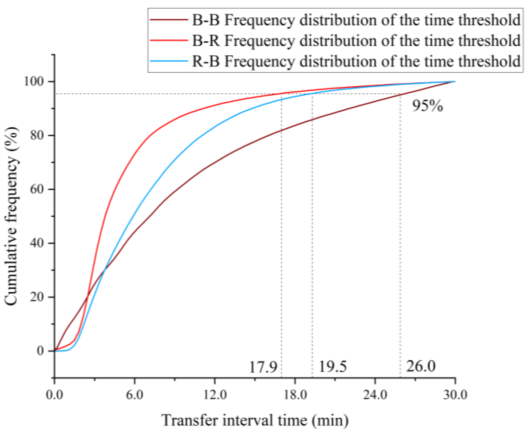
Figure 1. Setting of time thresholds in Hangzhou’s combined travel chain data.
Ijgi 14 00281 g001
Figure 2. Flowchart of initial travel data processing.
Ijgi 14 00281 g002
Figure 3. Schematic diagram of constructing the confidence ellipse.
Ijgi 14 00281 g003
Figure 4. Study area.
Ijgi 14 00281 g004
Figure 5. Confidence ellipse for ID 6.
Ijgi 14 00281 g005
Figure 6. Activity space sizes for three different travel modes in grid no. 287.
Ijgi 14 00281 g006aIjgi 14 00281 g006b
Figure 7. Multimodal transportation residents’ activity space for combined metro–bus travel in Hangzhou.
Ijgi 14 00281 g007
Figure 8. Grid and district in Hangzhou.
Ijgi 14 00281 g008
Figure 9. The importance of features.
Ijgi 14 00281 g009
Figure 10. Partial dependence plot for distance to nearest metro station.
Ijgi 14 00281 g010
Figure 11. Partial dependence plot for distance to CBD.
Ijgi 14 00281 g011
Figure 12. Partial dependence plot for commercial POIs.
Ijgi 14 00281 g012
Figure 13. Partial dependence plot for GDP.
Ijgi 14 00281 g013
Figure 14. Geospatial effect of GEO.
Ijgi 14 00281 g014
Figure 15. Geospatial effect of the interaction between GEO and distance to the nearest metro station.
Ijgi 14 00281 g015
Table 1. The evolution of concepts and measurement methods for activity space.
Author(s) and YearCore Concept/ContributionMeasurement Method/Approach
Hägerstrand (1970) [17]Introduced the foundational concept of “space-time prisms” from time–geography, focusing on individual constraints.Conceptual framework for potential activity space under spatiotemporal constraints.
Newsome et al. (1998) [20]Emphasized commuters’ spatially constrained activity structures.Pioneered the use of elliptical models to statistically summarize the spatial distribution of activity locations.
Schönfelder & Axhausen (2003) [23]Proposed a method to approximate travelers’ actual activity ranges by linking travel paths to surrounding areas.Developed path buffer zones based on road network paths.
Buliung & Kanaroglou (2006) [21]Achieved more precise depictions by incorporating non-work activity locations anchored by household members.Utilized convex polygon models to delineate accessible spaces.
Yu & Shaw (2008) [27]Advanced visualization to overcome the limitations of 2D representations.Designed a 3D spatiotemporal GIS framework to visualize human activities in both physical and virtual spaces.
Zhou et al. (2015) [24]Focused on identifying functionally important nodes and analyzing spatiotemporal travel patterns in an urban network.Introduced the “Functional Crucial Network Location” (FCNL) concept using taxi trajectory data.
Table 2. Desensitized metro data in Hangzhou.
Card_IDArrival TimeArrival StationDeparture StationDeparture TimeRecord_ID
20883******0740001 November 2023 13:31Jiuhe Road StationWulin Square Station1 November 2023 13:54R580353
48801******4988001 November 2023 13:10Puyan StationChengzhan Station1 November 2023 13:40R549797
20880******6682001 November 2023 7:53Nanxingqiao StationJiangjin Road Station1 November 2023 8:05R2017405
Table 3. Desensitized bus data in Hangzhou.
Card_IDArrival TimeArrival StationDeparture StationDeparture TimeRecord_ID
31000******2825001 November 2023 11:16LiaojiaHangzhou Ecological Park1 November 2023 11:36B797670
31007******6555001 November 2023 19:08Liuxia NorthKechuang Road1 November 2023 19:47B13021
31007******00429001 November 2023 7:07Guanshan ParkHengshan Xia1 November 2023 7:38B92135
Table 4. Available travel chain data in Hangzhou’s Ring Expressway area.
Start_LngStart_LatEnd_LngEnd_LatID
120.215904130.18973507120.163086130.248307576
120.215904130.18973507120.231891330.234858856
120.215904130.18973507120.37706430.28894476
120.215904130.18973507120.145488930.28246066
120.215904130.18973507120.135378630.285598136
120.215904130.18973507120.144383430.310118786
120.215904130.18973507120.206632730.247167816
120.215904130.18973507120.428561630.237837986
120.215904130.18973507120.193270130.233202266
Table 5. Statistical description of variables.
VariablesDescriptionMeanMinMax
Dependent variable
Area of Activity SpaceArea of the confidence ellipse for each grid (km2)606.9210.001627.89
Socioeconomic attributes
GDPPer capita GDP in the grid (CNY/km2)62,928.44986753,4418
Built environment
Catering POINumber of catering POIs in the grid (counts)109.500.001197.00
Commercial POINumber of commercial POIs in the grid (counts)77.520.00858.00
Science and education POINumber of science and education POIs in the grid (counts)18.240.00152.00
Residential POINumber of residential POIs in the grid (counts)15.390.00116.00
Healthcare POINumber of healthcare POIs in the grid (counts)16.510.00232.00
Population densityPopulation density in the grid (pop)5153.76962.8722,241.18
Distance to CBDEuclidean distance from the grid center to the CBD (m)10,657.06232.5721,478.29
Number of Metro Stations within 3 km BufferNumber of metro stations within a 3 km buffer of the grid center (counts)11.750.0045.00
Bus stopsNumber of bus stops in the grid (counts)5.680.0022.00
Land use mixDegree of land use mix0.670.000.97
Distance to Nearest Metro StationDistance from the grid center to the nearest metro station (m)1360.6365.057481.26
Table 6. Model performance evaluation.
Training Set R2Test Set R2
XGBoost + GeoShapley0.5130.432
XGBoost (no GEO)0.3950.317
Random Forest0.3620.328
OLS0.1890.115
GAM0.2270.213
Disclaimer/Publisher’s Note: The statements, opinions and data contained in all publications are solely those of the individual author(s) and contributor(s) and not of MDPI and/or the editor(s). MDPI and/or the editor(s) disclaim responsibility for any injury to people or property resulting from any ideas, methods, instructions or products referred to in the content.