Automated Digitization Approach for Road Intersections Mapping: Leveraging Azimuth and Curve Detection from Geo-Spatial Data

Abstract

Effective maintenance and management of road infrastructure are essential for community well-being, economic stability, and cost efficiency. Well-maintained roads reduce accident risks, improve safety, shorten travel times, lower vehicle repair costs, and facilitate the flow of goods, all of which positively contribute to GDP and economic development. Accurate intersection mapping forms the foundation of effective road asset management, yet traditional manual digitization methods remain time-consuming and prone to gaps and overlaps. This study presents an automated computational geometry solution for precise road intersection mapping that eliminates common digitization errors. Unlike conventional approaches that only detect intersection positions, our method systematically reconstructs complete intersection geometries while maintaining topological consistency. The technique combines plane surveying principles (including line-bearing analysis and curve detection) with spatial analytics to automatically identify intersections, characterize their connectivity patterns, and assign unique identifiers based on configurable parameters. When evaluated across multiple urban contexts using diverse data sources (manual digitization and OpenStreetMap), the method demonstrated consistent performance with mean Intersection over Union greater than 0.85 and F-scores more than 0.91. The high correctness and completeness metrics (both more than 0.9) confirm its ability to minimize both false positive and omission errors, even in complex roadway configurations. The approach consistently produced gap-free, overlap-free outputs, showing strength in handling interchange geometries. The solution enables transportation agencies to make data-driven maintenance decisions by providing reliable, standardized intersection inventories. Its adaptability to varying input data quality makes it particularly valuable for large-scale infrastructure monitoring and smart city applications.

1. Introduction

Road infrastructure is vital for economic growth, facilitating passenger and freight transportation, while influencing safety, comfort, and costs. Effective maintenance and management enhance accessibility, mobility, and community development, necessitating integrated treatment plans for optimal road network performance [1]. Furthermore, the impact of road maintenance extends beyond immediate community benefits; it also aligns with broader sustainability goals outlined in the United Nations Sustainable Development Goals (SDGs) [2]. For instance, maintaining reliable infrastructure supports economic growth (SDG 8), contributes to building resilient infrastructure (SDG 9), promotes sustainable cities and communities (SDG 11), and well-maintained roads facilitate access to essential services such as healthcare, education, and employment opportunities, which are vital for improving the quality of life and reducing poverty levels. In contrast, poorly maintained roads can lead to increased travel costs, hinder service delivery, and elevate the risk of accidents, ultimately affecting community well-being and economic stability.

Data-driven road maintenance leverages Geographic Information System (GIS) technology to revolutionize road management and maintenance processes by integrating spatial data with operational planning. GIS serves as a powerful framework for road network management, offering systematic documentation and efficient data handling. By incorporating spatial and topological relationships among geo-referenced entities, GIS enhances the accuracy of road geometry, intersections, and associated attributes. With its advanced capabilities—such as thematic mapping, statistical analysis, decision support, network modeling, multi-database access—GIS enhances highway management and infrastructure development. Moreover, GIS provides intuitive visualization through spatially oriented maps, surpassing traditional tables and graphs in data interpretation. By displaying patterns and relationships in a geographic context, GIS enables users to analyze problems in relation to both space and time, improving situational awareness and supporting more effective decision-making [3]. Together, these GIS capabilities empower the development of digital road network models and optimize road infrastructure management through data-driven approaches. So, GIS technology supports a wide range of applications, including road maintenance [4], human mobility [5], transport planning [6], and emergency response [7].

In road maintenance projects, GIS serves as a flexible tool for managing road asset data through storage, retrieval, and analysis. A notable example is the GIS-based Intersection Inventory System (GIS-IIS) developed by the Illinois Department of Transportation. This system efficiently integrates diverse data sources, such as traffic signal details and multimedia resources, to create a detailed inventory of signalized intersections, demonstrating the powerful role that GIS can play in managing infrastructure data [8]. Moreover, there is an established research focus on using GIS for visualizing and integrating project data to address planning challenges in highway agencies. Key directions include supporting integrated planning, and leveraging geospatial visualization for developing spatial decision support systems [9,10,11,12]. Formalizing the prioritization process with GIS and decision analysis techniques is essential for sustainable transit infrastructure development. Some studies (e.g., [3,4,10,11]) have proposed GIS-based models for highway maintenance prioritization, incorporating pavement condition and other relevant factors. These models utilize GIS for visualizing data, managing information, and automating maintenance planning, improving overall efficiency and effectiveness. One of the main tasks in GIS, particularly for infrastructure projects (e.g., road maintenance management) and urban planning, is digitization. This process involves converting geographic features into digital formats for visualization, storage of related information, and analysis. It allows for the creation of vector data that represents real-world entities, such as roads, buildings, and boundaries, forming the foundation for numerous geospatial applications [13].

The manual digitization is a time-intensive process that requires significant human effort and resources. It often involves multiple users working on tasks such as tracing features, verifying data, and ensuring accuracy, which increases operational costs. Additionally, the reliance on manual effort can lead to inconsistencies and errors due to subjective interpretations. These limitations make automated digitization, particularly with advanced techniques like deep learning, an attractive alternative for reducing reliance on extensive manual work [14,15]. Recent advancements in automated techniques have significantly reduced the time and cost associated with this process, making it a highly efficient alternative to the traditionally costly and labor-intensive manual approach [14,15,16].

Automatic digitization using multi-source data and deep learning has become a prominent focus for segmenting roads, buildings, and trees, supporting applications such as urban planning, disaster response, and environmental monitoring [17,18,19]. Despite these advancements, the accuracy of digitization, particularly for intersections extraction, remains a critical limitation. Errors in segment extraction can propagate through workflows, impacting tasks such as quantity estimation and spatial analysis. Intersections, which often require precise geometry for reliable measurements, are especially challenging due to overlapping features, complex geometries, and varying data quality. Addressing these issues is vital to enhance the reliability of automated digitization systems and ensure their applicability across diverse domains.

To the best of our knowledge, existing research has investigated the detection of the positions of road intersections using either raster images or GPS trajectories [20]. For example, Chiang et al. [21,22] employed raster maps from various sources to detect road intersections, which served as the foundation for automatic road digitization. Considering that road maps are among the most commonly used map types and road layers are widely available across various geospatial data sources, the road network can be leveraged to integrate maps with other geospatial data. In [23], road footprint classification methods were applied to automatically extract road networks and to identify intersections from aerial images. With advancements in the Internet of Things (IoT) and Information and Communication Technologies (ICT), the availability of large-scale vehicle trajectory data has significantly increased, offering valuable opportunities for big-geospatial data analysis. This rich dataset can be utilized to detect road intersection points by analyzing characteristics within intersection areas, such as the clustering of turning points [24,25,26]. Zhang et al. [26] developed a deep learning algorithm based on YOLOv5 architecture for detecting road intersections using crowd-sourced data from vehicle trajectories. The approach successfully identifies the locations of road intersections with different shapes, but it does not map the shape of the intersections as a vector layer. The advancement of computing capabilities and the ability to process multi-source data has made the integration of diverse datasets a prominent research focus. Fusing multi-source data, such as OpenStreetMap (OSM) data, satellite imagery, aerial imagery, and GPS trajectories, serves as a catalyst for improving the accuracy of detecting road intersection points [15,17,27].

To contextualize the proposed methodology, we classify and compare existing road intersection detection approaches. These approaches can be broadly categorized as either geometry-based [22,23,24,25,28,29,30,31,32] or deep learning-based [15,26,27,33,34,35,36]. However, as illustrated in

Table 1. Comparison of existing approaches for road intersection analysis: detection, positioning and mapping.

Reference	Input Data	Output (Road Intersections)
		Detection	Positioning	Mapping
Hu et al. [23]	Aerial Images	✓	✓	×
Chiang et al. [22]	Raster Maps	✓	✓	×
Wang et al. [28]	Trajectories Data	✓	×	×
Li et al. [29]	Trajectories Data	✓	✓	×
Xie and Philips [30]	Trajectories Data	✓	×	×
Zhou et al. [31]	HR Satellite Images	✓	✓	×
Saeedimoghaddam and Stepinski [33]	USGS Historical Map	✓	×	×
Li et al. [15]	Satellite Images and Trajectories Data	✓	✓	×
Gao et al. [24]	Trajectories Data	✓	✓	×
Huang and Sharma [25]	Trajectories Data	✓	×	×
Liu et al. [27]	Trajectories Data and OSM	✓	×	×
Yang et al. [35]	Trajectories Data	✓	×	×
Yang et al. [34]	OSM	✓	×	×
Du et al. [32]	Trajectories Data	✓	✓	×
Zhang et al. [26]	Trajectories Data	✓	×	×
Hetang et al. [36]	Satellite Images	✓	×	×
Proposed Method	Geospatial Vector Data	✓	✓	✓

, prior studies have primarily focused on identifying intersection positions, with significantly less attention given to their detailed spatial mapping.

While prior research has extensively addressed intersection detection in GIS, a critical gap remains in precisely mapping intersection geometries, including boundary delineation, topology, and compliance with road management standards. The proposed work bridges this gap by advancing beyond mere positional detection of road intersections to delineate geometric structures of the intersection (i.e., digitizing intersections) with high fidelity, adhering to road management and maintenance standards. This approach simultaneously resolves topological inconsistencies (e.g., overlaps and gaps) inherent in manual digitization processes. These digitized intersection maps are crucial for documenting road condition analysis after road surveys, calculating quantities and costs relevant to the road management and maintenance processes, and prioritizing the most necessary roads that require maintenance. In this work, the challenges of mapping road intersections are addressed by incorporating geometry computation principles based on land surveying, providing an efficient solution that reduces time and costs. By leveraging azimuth calculations and geometric methods, this approach enhances the extraction of intersections and other complex features, minimizing errors from overlapping elements, intricate geometries, and inconsistent data quality. It not only improves the reliability of automated digitization systems but also broadens their applicability across diverse domains by significantly reducing manual effort.

2. Methodology

This section outlines the methodology employed for automating the digitization of road intersections and assigning corresponding unique identifiers (IDs). It leverages computational geometry, spatial data integration to ensure precise mapping, achieve accurate results, and minimize manual intervention. The methodology consists of multiple structured main phases, as shown in Figure 1, to facilitate the accurate extraction and representation of intersections.

The methodology begins with preparing the spatial layer by loading and preprocessing datasets to ensure topological consistency. The input layers include the main street network and regional polygons, which represent the enclosed areas formed by intersecting main streets. Next, the azimuth computation phase determines the directional alignment of road segments, which helps in detecting key transitions (Corners and road fillets). The corner and fillet detection phases identify sharp corners and curved transitions. Buffers are then generated around corners and Points of Intersection (PIs) of fillets to define intersection influence areas. Then, tangents are generated along the dissolved buffer edges to enclose and define the intersection boundaries in the transverse directions of the intersecting roads. A convex hull is created to encapsulate key transition points, followed by a geometry difference computation to isolate precise road intersections. Finally, unique IDs are assigned to the extracted intersections for systematic integration into the spatial database. These structured phases automate the digitization of road intersections, and the following sections provide definitions of some acronyms used, along with a detailed explanation of each phase and the substeps involved in achieving the objectives of this study.

2.1. Definitions

Before delving into the detailed explanation of the methodology, this subsection provides definitions of key terms used to describe the processes involved in road intersection digitization:

• Region: A polygonal area formed between the intersecting main streets, representing the enclosed space surrounded by road segments. Each region is assigned a unique identifier called REGION_NO.
• Azimuth: An angle measured clockwise from the north to a line (e.g., a road segment or a segment of a region boundary represented as a polyline), defining its orientation.
• Key Transition: A Critical geometric features where road direction or curvature changes, such as corners or fillets.
• Corner: A Sharp angle points where two successive segments meet, serving as a type of key transition that forms the intersection.
• Fillet: A rounded transitions between intersecting roads, often designed using a specific radius to facilitate smoother vehicle turns and reduce sharp cornering.
• Tangents of Fillets: Straight lines extend from both ends of a fillet (a smooth connecting curve), defining its direction and ensuring a smooth transition between adjacent segments.
• Point of Intersection (PI): The theoretical intersection points of the tangents of fillets if extended.
• Point of Curvature (PC): The point where the curve begins (transition from tangent to curve).
• Point of Tangency (PT): The point where the curve ends and returns to a tangent.
• Dissolved Buffers: A single merged buffer encompassing multiple overlapping buffers around intersecting roads.
• Convex Hull: The smallest enclosing shape that contains all key transition points of an intersection.
• GeoDataFrame: A spatially-enabled tabular data structure that extends the capabilities of a traditional DataFrame by incorporating geospatial data.

2.2. Proposed Digitization Approach

In this work, a Python script is deployed, utilizing several libraries for geospatial data processing and analysis. $GeoPandas$ facilitates spatial data handling, while $Shapely$ supports geometric operations, including $unary\_union$, $linemerge$, and $nearest\_points$, along with geometry types such as $Point$, $LineString$, and $Polygon$. $WKT$ from $Shapely$ aids in geometry conversion. $NumPy$ and $Math$ provide numerical and trigonometric computations, while $Pandas$ manages attribute data. $Folium$ enables interactive map visualization, and $Webbrowser$ and $OS$ handle system interactions. These specialized libraries ensure efficient spatial analysis, seamless data processing, and interactive visualization, enhancing the accuracy and usability of geospatial datasets.

The following subsections provide a detailed explanation of the substeps in the following subsections, as presented in Figure 2, within the main phases presented in Figure 1.

2.2.1. Preparing the Spatial Layer

The preparation of the spatial layer involves loading and preprocessing the dataset to ensure topological consistency and spatial accuracy. A crucial step in this process is verifying the Coordinate Reference System (CRS) of the dataset, ensuring it is EPSG:32637, which corresponds to UTM Zone 37 North based on the WGS 84 datum. This CRS ensures precise spatial representation, maintaining accurate distance and area measurements. Then, data cleaning and error correction are performed to remove duplicate or overlapping geometries while fixing topological issues such as gaps and self-intersections. Following this, attribute standardization is carried out, ensuring fields are properly labeled, redundant attributes are removed, and the dataset is optimized for performance. Finally, topology validation is conducted to check connectivity within the street network, ensuring that intersections are correctly snapped and region polygons are fully enclosed. These preparatory steps collectively enhance the accuracy, consistency, and usability of the spatial data, supporting reliable analyses in road network management.

2.2.2. Azimuth Computation

After the data preparation step, one of the most pivotal phases of this work begins. Azimuth computation is fundamental in plane surveying, involving the determination of a line’s directional angle relative to the north direction (0°), measured clockwise from 0° to 360°. This method is widely used in surveying, navigation, and road network analysis. Algorithm A1 was implemented to calculate the azimuth for the segments forming the region’s boundaries, which also define the adjacent roads.

2.2.3. Detection of Fillets in Region Boundaries

Fillets are a key transition feature, as defined in Section 2.1, representing a rounded connection between intersecting roads. Commonly, curved or rounded transitions, when digitized manually, are represented either as a direct curve formed by three points or as multiple smaller segments approximating a smooth transition. To detect these curves, Algorithm A3 is applied based on the following two main steps.

• Radius Calculation and Curve Detection

This step is based on analyzing the local curvature of polygon boundaries using the circumradius of triangles formed by consecutive triplets of points. For each three consecutive points $(p_1,p_2,p_3)$, the Euclidean distances between them are computed as $a= \parallel p_2-p_1\parallel$, $b= \parallel p_3-p_2\parallel$, and $c= \parallel p_1-p_3\parallel$. The semi-perimeter is then calculated as follows:

$$s={\displaystyle \frac{a+b+c}{2}}$$

(1)

followed by the computation of the triangle’s area using Heron’s formula, expressed as follows:

$$\mathrm{Area}=\sqrt{s(s-a)(s-b)(s-c)}$$

(2)

If the area is nonzero, the circumradius is computed using the following formula:

$$R={\displaystyle \frac{a\times b\times c}{4\times \mathrm{Area}}}$$

(3)

As shown in Algorithm A3, the process of detecting curves in a polyline of region boundary involves iterating through consecutive points and analyzing their geometric properties. For each segment, the circumradius is computed to assess curvature, along with segment lengths to ensure they meet predefined criteria. Multi-part geometries are handled separately by processing each sub-geometry individually. Curved segments that satisfy the curvature and length thresholds are identified and stored as distinct geometric features, while maintaining their associated $REGION\_NO$. The adjacent curve segments within each region are merged to form continuous geometries while preserving their total length. The features are then sorted in counter-clockwise order on the basis of their spatial relationship to the region’s centroid. Finally, unique identifiers of detected fillets are assigned according to the sorted order, ensuring a structured and meaningful labeling system for further spatial analysis.

• Fillets Filtering Based on Street Network

This process starts by computing a unit perpendicular vector for each line segment of fillets, ensuring the buffer expands symmetrically in both directions. Using this vector, a flat directional buffer is generated by shifting points along the perpendicular direction, forming a polygon around the original fillet. Then, the buffered features are analyzed for intersections with a street network, identifying those that overlap multiple streets. Only buffers intersecting more than one distinct street are retained, while others are removed to ensure the dataset captures meaningful connections between fillets and multiple streets. The intersecting street numbers are extracted and stored as attributes for each fillet feature.

• Related Elements Detection for Fillets

To generate point features and fillet tangents from the given geometries, the process begins by grouping the data based on a specific region attribute. The segments within each region are then sorted in a clockwise order around the region’s centroid. For each segment, key points are extracted, including the start (PCs) and end points (PTs), as well as the centroid, which is projected onto the segment’s geometry. Descriptive labels are assigned to these points based on their sequence within the region. Each point is further associated with a unique identifier and a region reference. Finally, all extracted point features are compiled into a new GeoDataFrame while preserving the original coordinate reference system, as detailed in Algorithm A4.

2.2.4. Corners Detection

A corner represents a key transition in a region’s boundary, which can be modeled and detected when there is a significant change in azimuth or a notable deviation in the internal angle between two consecutive segments. This can be achieved by applying Algorithm A5. The internal angle between two consecutive segments is computed based on their azimuth values using the following equation:

$${\varphi }_{\mathrm{internal}}=\left({\theta }_{A{Z}_1}+{180}^{\circ }-{\theta }_{A{Z}_2}\right)mod{360}^{\circ }$$

(4)

where ${\theta }_{A{Z}_1}$ and ${\theta }_{A{Z}_2}$ are the azimuths of two consecutive segments, the result is constrained within $0^{\circ }$ to ${360}^{\circ }$ using the modulo operation.

The detected corners are classified into convex or concave corners based on the following criteria:

$$\mathrm{Corner}\mathrm{Type}=\left\{\begin{array}{c}\mathrm{Convex},{\varphi }_{\mathrm{internal}}<{180}^{\circ }\hfill \\ \mathrm{Concave},\mathrm{otherwise}\hfill \end{array}\right.$$

(5)

Furthermore, each detected corner is buffered by 50 m, and the number of intersecting streets is counted; corners intersecting only a single street are discarded to ensure that only significant corners are retained at true street intersections.

2.2.5. Buffer Generation and Tangent Origin Extraction

As part of automatic road intersection digitization, buffers are generated around key transition points, including road corners and Points of Intersection (PIs) of curves. In this step, a buffer with a radius of 50 m is generated around each key transition point to ensure adequate spatial coverage based on predefined criteria. This buffer size aligns with required intersection criteria used in road management and maintenance.

To maintain spatial consistency, overlapping buffers belonging to the same intersection are merged. This prevents fragmentation and ensures intersections are represented as unified spatial entities. The merging process involves identifying overlapping buffers with common intersecting streets and dissolving them into a single feature, preserving connectivity and structural integrity, as detailed in Algorithm A6.

2.2.6. Tangent Generation and Filtering

After extracting the origin points of the tangents at the intersection of the buffers with the road boundaries (which constitute the region edges), Algorithm A7 generates and filters the tangents. This process yields lateral boundaries that intersect orthogonally with the road’s longitudinal axis, thereby defining the intersection perimeter. The algorithm ensures geometric validity by retaining only those tangents that maintain approximate perpendicularity (≈90°) relative to the intersecting streets, while automatically discarding non-essential segments. When multiple tangent candidates exist, the selection process prioritizes the option exhibiting the closest alignment to true perpendicularity.

2.2.7. Convex Hull Application and Road Intersection Extraction

Our intersection extraction methodology implements Algorithm A8 through a sequential computational process. Initial convex hull construction around dissolved buffers incorporates multiple geometric primitives—specifically tangents, derived intersection points between filtered tangents and region boundaries, corners, and fillets. Subsequent geometric differencing between these convex hulls and the region Layer yields precise road intersection delineations. This approach ensures topologically robust representations by systematically resolving common manual digitization artifacts, including polygon overlaps and sliver gaps that plague manual processing methods. Figure 3 visually demonstrates this improvement through comparison, where the orange-outlined polygon reveals how conventional approaches introduce topological imperfections at intersections, while our method preserves geometric integrity through rigorous computational treatment.

2.2.8. Assign Unique ID for Generated Roads’ Intersections

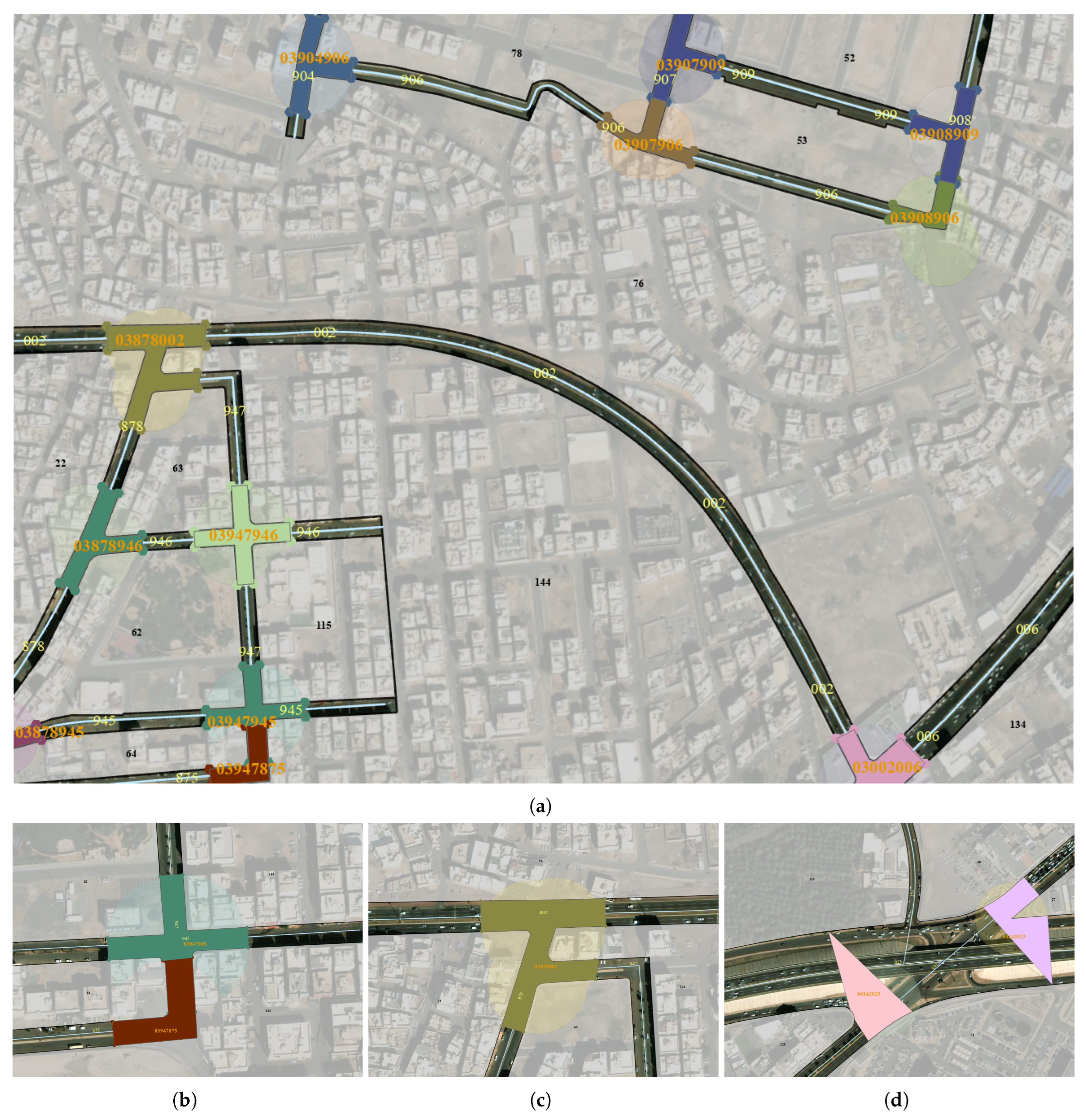
Intersections within a road network are systematically identified and assigned unique identifiers based on intersecting streets and their orientation. Each intersection is analyzed by extracting intersecting streets, determining the containing municipality, and computing aspect ratios to classify streets as North-South (NS) or East-West (EW). The primary NS and EW streets are identified based on maximum and minimum aspect ratios, respectively. Finally, a unique ID for road intersection is generated by concatenating the municipality ID (i.e., $MUNIC\_ID$) with the IDs (i.e., $MAIN\_ID$) of the selected NS and EW streets. Detailed steps are shown in Algorithm A2.

3. Experimental Results and Discussion

This section presents the data description, experimental results, and performance analysis of the automatic digitization method, evaluated through three case studies. The first two case studies focus on spatial vector data (street centerlines and region layers) from Al Madinah Al Munawwarah, manually digitized and quality-checked to ensure accuracy. The third case study examines a zone in Chengdu, China, using OpenStreetMap (OSM)-sourced spatial vector data, with further details provided in the relevant subsection. The results compare the automatic method’s accuracy against manual digitization, followed by a discussion of key challenges and performance insights.

3.1. Data Description

Before presenting and discussing the results, this section provides a description of the data used in this research, which served as the basis for mapping road intersections and validating the results by comparing the final outcome to the ground truth of road intersections.

3.1.1. Case Study 1

The study area is located in the center of Al Madinah Al Munawwarah, specifically in the area between Al-Masjid An-Nabawi–The Prophet’s Mosque (SAWS) and King Abdullah bin Abdulaziz Road (commonly known as the Second Ring Road). This study relies on the region layer and the main streets layer. The region layer, mentioned in Section 2.1, contains irregular and complex shapes, making the identification and delineation of road intersections a challenging task that requires careful handling. This layer includes data for approximately 150 features (i.e., regions) and is considered the base map in this study. The dataset was obtained as a shapefile and was manually digitized. The main streets layer—comprising roads with a width of 40 m or more—was manually digitized and subjected to stringent quality control (QC) procedures to ensure data reliability. While similar road data could theoretically be sourced from open-access platforms like OSM, this study relied exclusively on the manually digitized and verified dataset to guarantee accuracy and consistency. This dataset comprises a total of 157 main streets (i.e., centerlines).

3.1.2. Case Study 2

This subsection presents an experimental evaluation of automated intersection delineation outputs for an additional case study in Al-Madinah Al-Munawwarah. The analysis utilizes vector geospatial data comprising two primary layers: (1) a street network layer (centerlines) containing approximately 80 main streets represented as polylines, and (2) a region layer consisting of 70 polygons surrounded by an additional boundary polygon. All datasets were manually digitized following the same methodology used in the first case study. The study area encompasses eastern Al-Madinah Al-Munawwarah, bordering Al-Aqool Municipality, representing a typical new urban configuration. This location was selected to evaluate the method’s robustness across varying intersection densities and spatial patterns.

3.1.3. Case Study 3

This case study was conducted in an area located within Chengdu’s first ring road - the capital of Sichuan Province in southwest China. Chengdu represents a rapidly developing urban center characterized by a mixed urban/rural landscape and complex road networks typical of major Chinese cities. For this case study, we utilized OSM road network data instead of manually digitized road layers used in previous studies. While this open-source data offers significant advantages, it has limitations including missing street names for some road segments. Nevertheless, OSM remains one of the most valuable open geospatial data sources, particularly for road network analysis research [27,34,37,38].

As previously mentioned, we focused on road network within the first ring road. The data was filtered to include only primary, secondary, and tertiary road classifications, excluding all unnamed streets. The OSM dataset contains multiple features for the same street, so we dissolved the streets using the column named “name”. To ensure consistency with the street layers in the previous two case studies—and to prepare it for code execution with matching column names—we added a new column called “$MAIN\_NO$” to the OSM dataset. This assigns each unique street name a consistent 3-digit ID across the entire dataset. For the region layer, manual digitization was performed using OSM tiles at a 1:3000 scale to maintain a consistent viewport for the interactive map of OSM features. This process generated approximately 50 distinct regions within Chengdu’s first ring road area, collectively enclosed by a single additional boundary polygon.

It is worth noting that such data—used in the three case studies—can also be generated using GEOAI algorithms applied to satellite imagery. For example, Esri has developed deep learning tools capable of extracting blocks (i.e., regions) and streets from high-resolution (1-m) aerial or satellite imagery. We have evaluated the accuracy of automatically extracted road intersections based on the ground truth data. The ground truth data consists of manually digitized road intersections that have been reviewed and quality-checked.

3.1.4. Results and Discussion

This section demonstrates the algorithm execution outputs for study cases. Figure 4 presents the features generated after applying the four algorithms (Algorithms A1, A3, A4, and A5) used for detecting corners and identifying road fillets based on the azimuth computation of road border segments. To ensure better visualization of the results, the Figures do not display the entire study area but rather focus on a specific part with higher resolution. Figure 4a displays the detected corners as red square points and the detected fillets as orange polylines. Additionally, cyan points represent detected corners that are later excluded due to overlap with the fillets. To optimize performance and reduce redundancy, this exclusion step is directly incorporated into the corner detection algorithm (Algorithm A5), preventing duplicate buffering of key transition features in the same location. Although not mandatory, this optimization helps minimize computational time for subsequent algorithms and processing steps.

Figure 4b shows the ends of the detected fillets, where the PCs are represented as green triangle points and the PTs as red triangle points. These points are used to determine the fillet tangents, as shown in Figure 4c. These tangents are then extended to obtain the PIs of the fillets (see Figure 4d), which are key points of the fillets and key points that are analogous to the detected corner points used later for identifying intersections. Figure 4d displays the PIs of the fillets as circular dark blue points. Additionally, cyan points surrounded by the red circle and its corresponding buffer will be excluded in Algorithm A6 because they do not belong to normal feature key transitions (such as fillets or corners). In other words, they do not represent essential elements of a road intersection. From Figure 4a, it can be seen that the source fillet of some excluded points is generated at locations where the acceleration/deceleration lanes (surrounded by a red rectangle) or the emergency parking lanes, which are located in the middle of the road. Although these meet the conditions for detecting curves, they do not satisfy the conditions for road intersections in the subsequent algorithm (Algorithm A6) and will therefore be excluded later. Furthermore, the cyan points, whether representing corners or PI points, are surrounded by dark red rectangles and will also be excluded. Although they meet the conditions of Algorithm A5 and Algorithm A3, they will be removed along with their buffers based on the criteria of Algorithm A6.

Figure 5 presents the results obtained after applying Algorithm A6, which processes the key transition points, including both corners and PI points.

It is important to note that the radius of the buffer in Algorithm A6 is smaller than the one used in Algorithm A3. The purpose of the larger buffer in Algorithm A3 is to initially capture as many fillets as possible, ensuring comprehensive detection. In contrast, Algorithm A6 refines the results by filtering out unnecessary elements, leading to a more precise representation of the relevant intersection features. Figure 5a illustrates the buffers surrounding key transition elements. The buffers associated with detected corner points are shaded in light red, while those corresponding to detected PIs are depicted in sky blue.

As observed in Figure 5a, the yellow buffer represents an anomaly, as previously discussed. It is generated around points derived from fillets near acceleration and deceleration lanes. It is evident that the corresponding PI point is significantly distant from the fillet itself and, consequently, far from the actual intersection. As a result, this buffer can be disregarded since it overlays with only a single road, making it irrelevant for intersection identification and leading to its exclusion from the following processing steps. Additionally, a buffer outlined in cyan exhibits similar characteristics to the previously mentioned cases. However, unlike the yellow buffer, it is not excluded in the next steps of Algorithm A6. This is because it is located near a road intersection and intersects with multiple roads, making it a valid candidate for further analysis. It can also be observed in Figure 5a that the orange buffer, enclosed by a dark red rectangle, corresponds to a buffer associated with a detected corner. Although this buffer overlays with two roads, these roads do not intersect at a common point. Therefore, it is excluded, as it does not meet the criteria for identifying an intersection. Regarding the second buffer, when a smaller radius is used, it only overlaps with a single road. As a result, it does not proceed to the next steps for intersection detection. In Figure 5a, clusters of overlapping buffers can be observed, where these buffers coincide with the same intersecting roads. These overlapping buffers are dissolved to form a single feature, representing a unified intersection area. To ensure clear visualization, each cluster is displayed in a distinct color to differentiate it from the others, particularly neighboring clusters. Finally, points representing the intersections of buffers with road boundaries are generated. These points, shown in red, serve as seed points for generating tangents.

After obtaining the seed points (tangent points), Algorithm A7 was applied to generate tangents that define the boundary of the relevant road intersection area. Figure 6a illustrates all the tangents generated from the tangent points of various dissolved buffers. Figure 6b shows the remaining tangents after filtering, retaining only those that intersect and are nearly perpendicular to the relevant roads for each dissolved buffer. Following this filtering step, the remaining tangents were split at their intersection points with the region’s boundaries (i.e., road boundaries) to keep only the segments within the road corridor, as shown in Figure 6c, since these segments define the intersection limits. Finally, after executing the last step of Algorithm A7, the most perpendicular tangents were selected. In cases where multiple adjacent tangents were found within a distance of less than 50 m (half the buffer radius), only one tangent was retained at the intersection boundaries per intersection leg to prevent the intersection area from extending along different road legs beyond their natural intersection limits, as depicted in Figure 6d.

Figure 7 presents some results obtained after applying Algorithm A8. In Figure 7a, the extracted points from the endpoints of the final segments generated by the previous algorithm are displayed. The colors of these points are distinguished for each dissolved buffer to facilitate visualization. It is noticeable that there are small-sized points scattered along the outer boundary of the regions. These points represent the vertices that form the regions and appear in faint orange, except for the more significant vertices, which are used to determine the optimal shape of the convex hull. These crucial vertices are those that overlay with the corresponding dissolved buffer and are shown in sky blue. Subsequently, Graham’s Scan method is applied in part B of Algorithm A8 to generate the convex hull from the extracted points. Examples of the resulting convex hulls are shown in Figure 7b.

Figure 8a represents a sample of the final output of the automatic road intersection extraction process. In Figure 8b, two separate intersections are displayed, but there is an overlap between them. This overlap is not problematic from an algorithmic extraction standpoint—it actually represents the ideal output according to the designed approach. However, in practical applications, such as industrial use cases, this overlap may need to be adjusted. A refinement can be made by positioning the dividing line between the intersections at the midpoint of the overlapping area. This ensures that the overlapping space is not counted twice, improving accuracy for real-world implementation. In this case, the two intersections remain separate because the dissolved buffers for each intersection contain different sets of intersecting streets. In contrast, Figure 8c shows a different scenario where two intersections are merged into one. This occurs when the intersections are close together, and the buffers of one intersection overlap with those of another, covering intersecting streets from both groups. As a result, they are treated as a single intersection. The third case, shown in Figure 8d, occurs in large interchange intersections. Here, the fillet radius is too large, resulting in minimal overlap between buffers. Since the overlap percentage is small, it affects the efficiency of intersection extraction.However, such cases are rare and can be easily modified manually.

It is worth mentioning that Figure 8 demonstrates how the automatically delineated intersections exhibit neither overlaps nor gaps with adjacent region boundaries. This precise alignment with the regional edges represents a significant advantage over manual digitization (see Figure 3, where frequent topological errors (e.g., gaps and overlaps) typically require multiple revisions during quality control.

3.1.5. Evaluation Metrics

The evaluation of the extracted and delineated road intersections is conducted by comparing the results of the proposed approach with manually prepared ground truth data, utilizing four quantitative evaluation metrics [39]. The Mean Intersection over Union $mIoU$ (Equation (6)) is employed to measure the ratio of the intersection area to the union area between the automatically detected intersections and the ground truth. The metric ranges from 0, indicating low accuracy, to 1.0, representing high accuracy. The Completeness $C_m$ (Equation (7)) is used to quantify the ratio of the intersection area to the total area of the ground truth, with higher values indicating more comprehensive detection. Conversely, the Correctness $C_r$ (Equation (8)) is calculated as the ratio of the intersection area to the total area of the automatically reconstructed intersection, where higher values correspond to greater accuracy. Finally, the $F_1$ score (Equation (9)) is utilized as a comprehensive metric that integrates both Completeness and Correctness, providing a balanced measure of detection performance.

$$mIoU={\displaystyle \frac{1}{n}}\sum _{k=1}^n{\displaystyle \frac{Are{a}_{computed}\cap Are{a}_{groundtruth}}{Are{a}_{computed}\cup Are{a}_{groundtruth}}}$$

(6)

$$C_m={\displaystyle \frac{Are{a}_{computed}\cap Are{a}_{groundtruth}}{Are{a}_{groundtruth}}}$$

(7)

$$C_r={\displaystyle \frac{Are{a}_{computed}\cap Are{a}_{groundtruth}}{Are{a}_{computed}}}$$

(8)

$$F_1=2{\displaystyle \frac{C_r{C}_m}{C_r+C_m}}$$

(9)

The detection performance of the proposed methodology was quantitatively assessed using a ground truth dataset comprising 228 for Case Study 1, 133 for Case Study 2, and 79 for Case Study 3 verified intersections, as shown in Figure 9a, Figure 10a and Figure 11a, repectively, with a colorscale indicating IoU, where green represents high IoU and red indicates low IoU. Our method extracted and delineated 232 intersections for Case Study 1, 125 for Case Study 2, and 76 for Case Study 3, including some cases (highlighted in red in the output data) that do not correspond to real-world intersections in the ground truth. These discrepancies occur primarily due to artificial structures—such as tunnels, bridges, and complex roadway designs—which may appear as intersections in spatial datasets but do not permit actual vehicle movement interactions at those locations. Among the reference intersections, the system failed to detect three intersections due to their geometric characteristics, as highlighted in the third case (Figure 8d) in the discussion section.

The box plot visualization demonstrates consistent performance across all metrics (as shown in Figure 9b). The comprehensive evaluation employed four key performance indicators: Mean Intersection over Union (mIoU) = 0.88, Detection Correctness = 0.94, Detection Completeness = 0.93, and Composite F-factor = 0.93. The proposed method was validated on addtional two distinct case studies to assess its effectiveness and performance consistency (as shown in Figure 10 and Figure 11). Quantitative evaluation revealed high segmentation accuracy, with mean Intersection-over-Union (mIoU) scores of 0.88 (Case Study 2) and 0.85 (Case Study 3). Correctness scores further demonstrated reliability, reaching 0.94 for Case Study 2 and 0.90 for Case Study 3. Additionally, the method achieved a completeness score of 0.9 for both datasets, indicating robust detection capability. The F-factor, a combined measure of precision and recall, exceeded 0.9 in all evaluations. These results collectively confirm the method’s robustness and generalizability across diverse assessment scenarios.

3.1.6. Limitations and Future Considerations

The current methodology, while effective in algorithmic extraction, presents certain limitations in practical applications. First, overlapping intersections may require post-processing adjustments, such as midpoint division, to avoid double-counting in real-world scenarios. Second, when intersections are in close proximity, the algorithm may merge them into a single entity. Third, large interchange intersections pose a greater challenge in delineation compared to standard cases due to suboptimal fillet radius settings, though such occurrences are infrequent. To address these limitations, future research should focus on three key improvements: (1) developing adaptive algorithms that integrate diverse geospatial datasets to dynamically optimize buffer parameters, enhancing accuracy across various intersection types and scenarios; (2) implementing advanced geometric processing to precisely identify and redelineate intersecting features, eliminating double-counting artifacts; and (3) incorporating GeoAI techniques for automated feature extraction (including roads and region layers) to significantly reduce manual intervention in the intersection identification process.

4. Conclusions

Well-maintained roads are essential for economic growth, urban resilience, and sustainable development, ensuring businesses operate efficiently and communities have reliable access to essential services. Effective infrastructure management enhances transportation networks, reduces traffic congestion, and improves road safety. As high-traffic areas, intersections require frequent maintenance and strategic planning to enhance traffic flow, improve safety, and allocate resources efficiently. Proper documentation plays a crucial role in prioritizing repairs, optimizing infrastructure investments, and supporting urban planning by integrating public transport and future developments. A key aspect of documentation is the spatial layer, which serves as a storage system for essential information and attributes. To enhance accuracy and efficiency, this study proposes a framework for automatic digitization of road intersections using GIS and computational geometry techniques, incorporating azimuth and curve detection.

While prior research has focused primarily on intersection detection, our approach advances beyond conventional methods by both delineating and mapping road intersection boundaries while preventing topological errors (e.g., overlaps and gaps) that typically occur during manual digitization processes. This automated approach delivers faster results while reducing human error and improving efficiency. Unlike manual digitization—which is slow, inconsistent, and subjective—the system standardizes workflows to produce reliable data, ensuring consistency and accuracy across different geographic locations. Additionally, assigning unique identifiers to digitized road intersections based on predefined criteria enables systematic organization and easy retrieval of intersection data, which is essential for infrastructure planning and decision-making. By eliminating the risk of duplicate identifiers—an issue commonly detected during quality control—the proposed approach enhances data integrity and consistency and ensures the creation of unique and accurate identifiers, in contrast to manual data entry, which is prone to such errors.

Across all three case studies, the method demonstrated consistent performance in intersection detection, achieving mean IoU scores of 0.85–0.88 and F-scores of 0.91–0.93. High correctness (0.90–0.94) and completeness (0.93–0.94) scores confirm its robustness in minimizing false positives while capturing true intersections. Notably, this performance was maintained despite using heterogeneous input data—including manually digitized street layers and OSM data across different cities—highlighting the method’s adaptability to varying data quality and urban contexts. These results validate the approach’s reliability for both simple intersections and complex roadway designs in real-world application

In conclusion, this study presents an innovative and efficient solution for automated road intersection mapping, addressing the limitations of traditional manual digitization methods. The GIS-driven approach enhances accuracy, reduces processing time, and demonstrates notable improvements in productivity for organizations involved in highway maintenance and management. By implementing this system, transportation agencies can significantly improve road safety, support better decision-making for road infrastructure management, and achieve long-term cost savings in infrastructure maintenance.

References

1. Yang, X.; Zhang, J.; Liu, W.; Jing, J.; Zheng, H.; Xu, W. Automation in road distress detection, diagnosis and treatment. J. Road Eng. 2024, 4, 1–26. [Google Scholar] [CrossRef]
2. Department of Economic Social Affairs. Global Sustainable Development Report. 2023. Available online: https://sdgs.un.org/gsdr (accessed on 10 April 2025).
3. Pantha, B.R.; Yatabe, R.; Bhandary, N.P. GIS-based highway maintenance prioritization model: An integrated approach for highway maintenance in Nepal mountains. J. Transp. Geogr. 2010, 18, 426–433. [Google Scholar] [CrossRef]
4. Consilvio, A.; Hernández, J.S.; Chen, W.; Brilakis, I.; Bartoccini, L.; Di Gennaro, F.; van Welie, M. Towards a digital twin-based intelligent decision support for road maintenance. Transp. Res. Procedia 2023, 69, 791–798. [Google Scholar] [CrossRef]
5. Miller, H.J. Modelling accessibility using space-time prism concepts within geographical information systems. Int. J. Geogr. Inf. Syst. 1991, 5, 287–301. [Google Scholar] [CrossRef]
6. Senousi, A.M.; Liu, X.; Zhang, J.; Huang, J.; Shi, W. An Empirical Analysis of Public Transit Networks Using Smart Card Data in Beijing, China. Geocarto Int. 2022, 37, 1203–1223. [Google Scholar] [CrossRef]
7. Ozbek, E.D.; Zlatanova, S.; Aydar, S.A.; Yomralioglu, T. 3D Geo-Information requirements for disaster and emergency management. Int. Arch. Photogramm. Remote Sens. Spat. Inf. Sci. ISPRS Arch. 2016, 41, 101–108. [Google Scholar] [CrossRef]
8. Sun, D.; Benekohal, R.F.; Girianna, M. GIS-based Intersection Inventory System (GIS-IIS): Integrating GIS, Traffic Signal Data and Intersection Images. 2005. Available online: https://rosap.ntl.bts.gov/view/dot/5535 (accessed on 1 April 2025).
9. Shah, M.I.; Sabri, A.; Sarif, A.S. Analysis of Pavement Maintenance Using Geographical Information System (GIS). Prog. Eng. Appl. Technol. 2023, 4, 942–948. [Google Scholar] [CrossRef]
10. Nautiyal, A.; Sharma, S. Condition Based Maintenance Planning of low volume rural roads using GIS. J. Clean. Prod. 2021, 312, 127649. [Google Scholar] [CrossRef]
11. Yunus, M.Z.B.M.; Hassan, H.B. Managing Road Maintenance Using Geographic Information System Application. J. Geogr. Inf. Syst. 2010, 2, 215–218. [Google Scholar] [CrossRef]
12. France-Mensah, J.; O’Brien, W.J.; Khwaja, N.; Bussell, L.C. GIS-based visualization of integrated highway maintenance and construction planning: A case study of Fort Worth, Texas. Vis. Eng. 2017, 5, 7. [Google Scholar] [CrossRef]
13. Longley, P.A.; Goodchild, M.F.; Maguire, D.J.; Rhind, D.W. Geographic Information Science and Systems; John Wiley & Sons: Hoboken, NJ, USA, 2015. [Google Scholar]
14. Jiao, C.; Heitzler, M.; Hurni, L. A novel framework for road vectorization and classification from historical maps based on deep learning and symbol painting. Comput. Environ. Urban Syst. 2024, 108, 102060. [Google Scholar] [CrossRef]
15. Li, Y.; Xiang, L.; Zhang, C.; Jiao, F.; Wu, C. A Guided Deep Learning Approach for Joint Road Extraction and Intersection Detection from RS Images and Taxi Trajectories. IEEE J. Sel. Top. Appl. Earth Obs. Remote Sens. 2021, 14, 8008–8018. [Google Scholar] [CrossRef]
16. Lichtner, W. Automatic digitization of conventional maps and cartographic pattern recognition. ISPRS Arch. 1988, 218–226. Available online: https://www.isprs.org/proceedings/Xxvii/congress/part4/218_XXVII-part4.pdf (accessed on 1 April 2025).
17. Wang, Z.; Xiang, L.; Liu, Z.; Wang, Z. Automatic Extraction of Roads From Multisource Geospatial Data Using Fusion Attention Network and Regularization Algorithm. IEEE Trans. Geosci. Remote Sens. 2024, 63, 5603517. [Google Scholar] [CrossRef]
18. Sertel, E.; Hucko, C.M.; Kabadayı, M.E. Automatic Road Extraction from Historical Maps Using Transformer-Based SegFormers. ISPRS Int. J. Geo-Inf. 2024, 13, 464. [Google Scholar] [CrossRef]
19. Ekim, B.; Sertel, E.; Kabadayı, M.E. Automatic road extraction from historical maps using deep learning techniques: A regional case study of Turkey in a German world war II map. ISPRS Int. J. Geo-Inf. 2021, 10, 492. [Google Scholar] [CrossRef]
20. Chen, B.; Ding, C.; Ren, W.; Xu, G. Automatically tracking road centerlines from low-frequency GPS trajectory data. ISPRS Int. J. Geo-Inf. 2021, 10, 122. [Google Scholar] [CrossRef]
21. Chiang, Y.Y.; Knoblock, C.A.; Chen, C.C. Automatic Extraction of Road Intersections from Raster Maps. In Proceedings of the GIS ’05: Proceedings of the 13th Annual ACM International Workshop on Geographic Information Systems, Association for Computing Machinery, Bremen, Germany, 4–5 November 2005; pp. 267–276. [Google Scholar] [CrossRef]
22. Chiang, Y.Y.; Knoblock, C.A.; Shahabi, C.; Chen, C.C. Automatic and accurate extraction of road intersections from raster maps. GeoInformatica 2009, 13, 121–157. [Google Scholar] [CrossRef]
23. Hu, J.; Razdan, A.; Femiani, J.C.; Cui, M.; Wonka, P. Road network extraction and intersection detection from aerial images by tracking road footprints. IEEE Trans. Geosci. Remote Sens. 2007, 45, 4144–4157. [Google Scholar] [CrossRef]
24. Gao, L.; Wei, L.; Yang, J.; Li, J. Automatic Intersection Extraction Method for Urban Road Networks Based on Trajectory Intersection Points. Appl. Sci. 2022, 12, 5873. [Google Scholar] [CrossRef]
25. Huang, T.; Sharma, A. Intersection Identification Using Large-scale Vehicle Trajectory Data. In Proceedings of the Proceedings of the Fifth International Conference of Transportation Research Group of India: 5th CTRG Volume 2; Springer: Berlin/Heidelberg, Germany, 2022; pp. 151–159. [Google Scholar] [CrossRef]
26. Zhang, Y.; Tang, G.; Sun, N. Detecting Road Intersections from Crowdsourced Trajectory Data Based on Improved YOLOv5 Model. ISPRS Int. J. Geo-Inf. 2024, 13, 176. [Google Scholar] [CrossRef]
27. Liu, Y.; Qing, R.; Zhao, Y.; Liao, Z. Road Intersection Recognition via Combining Classification Model and Clustering Algorithm Based on GPS Data. ISPRS Int. J. Geo-Inf. 2022, 11, 487. [Google Scholar] [CrossRef]
28. Wang, J.; Wang, C.; Song, X.; Raghavan, V. Automatic intersection and traffic rule detection by mining motor-vehicle GPS trajectories. Comput. Environ. Urban Syst. 2017, 64, 19–29. [Google Scholar] [CrossRef]
29. Li, L.; Li, D.; Xing, X.; Yang, F.; Rong, W.; Zhu, H. Extraction of road intersections from GPS traces based on the dominant orientations of roads. ISPRS Int. J. Geo-Inf. 2017, 6, 403. [Google Scholar] [CrossRef]
30. Xie, X.; Philips, W. Road intersection detection through finding common sub-tracks between pairwise GNSS traces. ISPRS Int. J. Geo-Inf. 2017, 6, 311. [Google Scholar] [CrossRef]
31. Zhou, T.; Sun, C.; Fu, H. Road information extraction from high-resolution remote sensing images based on road reconstruction. Remote Sens. 2019, 11, 79. [Google Scholar] [CrossRef]
32. Du, J.; Liu, X.; Meng, C. Road Intersection Extraction Based on Low-Frequency Vehicle Trajectory Data. Sustainability 2023, 15, 14299. [Google Scholar] [CrossRef]
33. Saeedimoghaddam, M.; Stepinski, T.F. Automatic extraction of road intersection points from USGS historical map series using deep convolutional neural networks. Int. J. Geogr. Inf. Sci. 2020, 34, 947–968. [Google Scholar] [CrossRef]
34. Yang, M.; Jiang, C.; Yan, X.; Ai, T.; Cao, M.; Chen, W. Detecting interchanges in road networks using a graph convolutional network approach. Int. J. Geogr. Inf. Sci. 2022, 36, 1119–1139. [Google Scholar] [CrossRef]
35. Yang, X.; Hou, L.; Guo, M.; Cao, Y.; Yang, M.; Tang, L. Road intersection identification from crowdsourced big trace data using Mask-RCNN. Trans. GIS 2022, 26, 278–296. [Google Scholar] [CrossRef]
36. Hetang, C.; Xue, H.; Le, C.; Yue, T.; Wang, W.; He, Y. Segment anything model for road network graph extraction. In Proceedings of the Proceedings of the IEEE/CVF Conference on Computer Vision and Pattern Recognition, Seattle, WA, USA, 16–22 June 2024; pp. 2556–2566. [Google Scholar] [CrossRef]
37. Senousi, A.M.; Zhang, J.; Shi, W.; Liu, X. A proposed framework for identification of indicators to model high-frequency cities. ISPRS Int. J. Geo-Inf. 2021, 10, 317. [Google Scholar] [CrossRef]
38. Boeing, G. Modeling and analyzing urban networks and amenities with OSMnx. Geographical Analysis. 2025. Available online: https://geoffboeing.com/share/osmnx-paper.pdf (accessed on 11 April 2025).
39. Ren, Y.; Li, X.; Jin, F.; Li, C.; Liu, W.; Li, E.; Zhang, L. Extracting Regular Building Footprints Using Projection Histogram Method from UAV-Based 3D Models. ISPRS Int. J. Geo-Inf. 2025, 14, 6. [Google Scholar] [CrossRef]
Figure 1. Main phases of road intersection digitization.
Ijgi 14 00264 g001
Figure 2. Detailed framework depicting the complete process of road intersection mapping.
Ijgi 14 00264 g002
Figure 3. (a) Potential topological artifacts in vector layers: sliver gaps and polygon overlaps; (b) representative cases where gaps and overlaps emerge during manual digitization.
Ijgi 14 00264 g003
Figure 4. Subplots illustrating the detection of corners and fillets based on azimuth computation of road border segments: (a) Detected corners (red squares) and fillets (orange polylines). (b) Ends of detected fillets, where PCs (green triangles) and PTs (red triangles) define fillet tangents. (c) Fillet tangents extended to determine PIs (dark blue polylines). (d) Identified PIs (dark blue circles) used for intersection detection, with cyan points representing non-essential transitions that are excluded in subsequent processing.
Ijgi 14 00264 g004
Figure 5. Results of Algorithm A6, illustrating buffers around key transition points. (a) Buffers around detected corner (light red) and PIs points (sky blue), with anomalies in other colors (executing Part A of Algorithm A6). (b) Overlapping buffers merged to form unified intersection areas, with red seed points indicating buffer intersections with road boundaries for tangent generation.
Ijgi 14 00264 g005
Figure 6. Results of Algorithm A7. (a) Initial tangents generated from tangent points of dissolved buffers. (b) Filtered tangents, retaining only those nearly perpendicular to roads. (c) Retained segments within the road corridor. (d) Final most suitable tangent segments.
Ijgi 14 00264 g006
Figure 7. Results of Algorithm A8. (a) Extracted points from the endpoints of the final segments, with distinct colors for each dissolved buffer. Significant vertices used for convex hull generation are highlighted in sky blue. (b) Resulting convex hulls generated using Graham’s Scan method.
Ijgi 14 00264 g007
Figure 8. (a) Sample output of the automatic road intersection extraction process. Cases of extraction limitations: (b) Overlapping sections between two separate intersections. (c) Merged intersections due to close proximity. (d) Large interchange.
Ijgi 14 00264 g008
Figure 9. Performance evaluation of the proposed intersection detection method through comparison between ground truth and detected intersections. (a) Spatial visualization of mean Intersection-over-Union (IoU) for detected road intersections, with high IoU values shown in green and low values in red. (b) Box plot of evaluation metrics: IoU, Detection Correctness, Detection Completeness, and F-factor For Case Study 1.
Ijgi 14 00264 g009
Figure 10. Performance evaluation of the proposed intersection detection method through comparison between ground truth and detected intersections. (a) Spatial visualization of mean Intersection-over-Union (IoU) for detected road intersections, with high IoU values shown in green and low values in red. (b) Box plot of evaluation metrics: IoU, Detection Correctness, Detection Completeness, and F-factor For Case Study 2.
Ijgi 14 00264 g010
Figure 11. Performance evaluation of the proposed intersection detection method through comparison between ground truth and detected intersections. (a) Spatial visualization of mean Intersection-over-Union (IoU) for detected road intersections, with high IoU values shown in green and low values in red. (b) Box plot of evaluation metrics: IoU, Detection Correctness, Detection Completeness, and F-factor For Case Study 3.
Ijgi 14 00264 g011