

Interactive Visualization for the GTFS and GTFS-RT Data of Budapest

Abstract
1. Introduction
Smart City and Mobility
2. Related Work and Our Research Objectives
2.1. Public Transport Services of Budapest
2.2. Research Objectives
- From a database theory perspective, we have a classic relational database stored in a ZIP file, which offers an efficient storage format thanks to its encoding scheme, resulting in a significant compression ratio. The GTFS file contains trip data for the next 30 days, and, according to the specification, changes are not recommended within 7 days of the planned trip dates. This allows trip planning applications to pre-process the data before users begin to query it intensively. GTFS-RT feeds provide real-time updates on vehicle positions, arrival time predictions, and alerts for detours and cancellations. Efficient utilization and processing of this data are crucial. To create a robust application capable of delivering real-time responses to user requests, it is essential to handle these file formats together. From a scientific standpoint, building a historical database that can be analyzed in different contexts is also of great interest.
- If geoinformatics perspectives are the focus, visualization and geospatial accuracy receive greater emphasis. For instance, it is crucial to ensure that the alignment and representation of the stops and the waypoints determining the route shapes are accurate.
- As a computer science-related topic, an efficient graph search algorithm is essential for planning trips between various stations, often involving multiple services and transfers. This challenge is significant because the graphs can extend not only across a city but also across entire continents.
- Consistent geovisualization requires consistent data; thus after collecting data we cleaned the data in the frame of a pre-processing;
- Building a historical dataset and using actual vehicle positions, which offers identification of the common features of disruptions and changes and the prediction of live arrival times with further traffic analysis.
3. Materials and Methods
3.1. Data Sources
3.1.1. Static Source (GTFS)
- agency.txt—The archive introduces two agencies having identifiers BKK and HEV. Agency BKK operates buses, trolleybuses, and trams, the other company MÁV-HÉV has replaced BKK for operating the suburban railway lines as the subsidiary of the company Hungarian State Railways (MÁV), referred as the agency MAV.
- calendar_dates.txt—As the GTFS specification states, the recommended way would be to specify patterns of services using entries calendar_dates.txt and calendar.txt together. However, archives use the alternate approach: each scheduled service is specified explicitly in the file calendar_dates. The schedule is available typically for the upcoming 1–2 month period.
- routes.txt—Different routes are identified using the following numbering scheme:
- Identifiers starting with the digits 0, 1, and 2 denote bus routes;
- Identifiers starting with the digit 3 denote tram routes;
- Identifiers starting with the digit 4 denote trolleybus routes;
- Identifiers starting with the digit 5 denote metro routes;
- Identifiers starting with the digit 8 denote boat services on the river Danube;
- Identifiers starting with the digit 9 denote night bus routes;
- Identifiers starting with the prefix VP (abbreviation for the Hungarian tram replacement expression) denote replacement bus services for tram routes, and identifiers starting with the prefix MP (abbrevation for the Hungarian metro replacement expression) denote replacement services for metro routes. Replacement services can be scheduled for various reasons, such as events and maintenance work;
- The schedules also contain additional routes for identifying the suburban railway services, special trips such as heritage trams, etc.
- shapes.txt—As one of the optional files, BKK’s GTFS archives contain the segments for representing the geoinformation for all variants of routes. This allows consumers to display the routes using various visualization techniques.
- stop_times.txt—This file contains one optional field: the field shape_dist_traveled gives the actual distance traveled along the associated shape.
- stops.txt—This file contains three optional fields and one non-standard field: fields stop_code, location_type, wheelchair_boarding, and location_sub_type.
- trips.txt—This file contains six optional fields: trip_headsign, direction_id, block_id, wheelchair_accessible, and bikes_allowed.
3.1.2. Realtime Sources (GTFS-RT)
- trip—Describes the Trip that the vehicle is serving. The corresponding TripDescriptor object contains the optional schedule_relationship field.
- position—Describes the current position of the vehicle. The corresponding Position object contains the optional fields bearing and speed.
- current_stop_sequence—The index of the current stop (that the vehicle is staying or is heading to).
- current_status—The status of the vehicle.
- timestamp—Moment at which the vehicle’s position was measured.
- stop_id—The ID of the vehicle’s current stop.
- license_plate: The license plate of the vehicle.
3.1.3. FUTÁR API
3.2. Collecting Data
- Period P1—The initial period started on 1 September 2023. At that moment, the FUTÁR API’s vehicles-for-location endpoint was invoked every 30 s to gather the live vehicle positions. We started to download the GTFS schedules twice a day: primarily, the state of the archive was fetched between 01:00 a.m. and 02:00 a.m.; however, a secondary fallback operation was also introduced between 01:00 p.m. and 02:00 p.m. In most of the cases, our service was able to download both versions; additionally, they were identical. In the case of differences, we kept the afternoon version of the schedule to consider the latest released content as next day’s schedule.
- Period P2—After a two-weeks long experience using the REST endpoint and our environment, we increased the frequency of the requests to 15 s, doubling the number of API calls within the same period starting on 18 September 2023.
- Period P3—On 29 April 2023, BKK deployed a new version of its API, introducing various limits on the queries. Thus, our previous calls—which queried the full area of Budapest for the vehicle positions—could not be used anymore. Realizing this change of the API, we discontinued the use of the REST API. Starting 4 May 2023, we replaced the old method by fetching the Vehicle Positions GTFS-RT feed for retrieving the live vehicle positions in its PB format instead of consuming the REST API’s JSON responses. This also introduced changes in the fetched data: additional properties are served using the standard format, and all the minor differences could be post-processed and unified between the multiple data sources.
- Period P4—Starting 21 July 2024, we increased the retrieval frequency by replacing the previous value of 15 s to 5 s. In parallel, we established the collection of the other two GTFS-RT feeds: the frequency of 600 s was introduced for the feeds Vehicle Positions and Service Alerts.
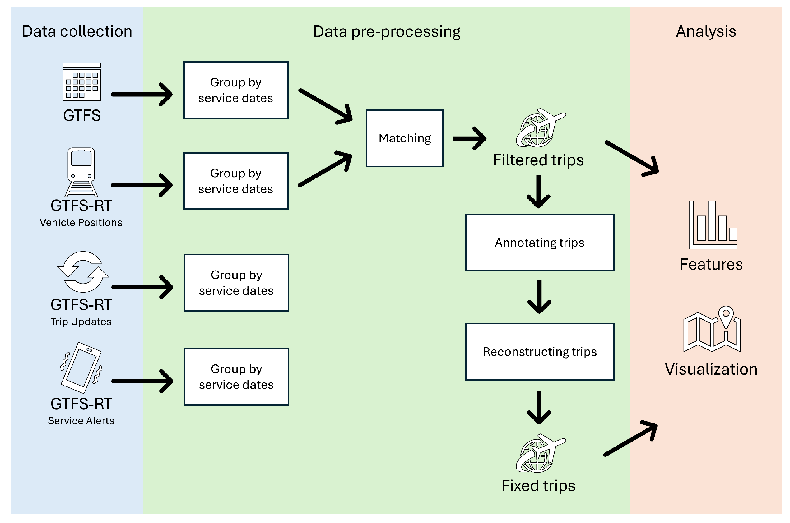
3.3. Pre-Processing Data
3.3.1. Cleaning the GTFS Schedules
- The bus, trolleybus, and tram lines served by the BKK agency serve as the basis for tracked routes; thus, we must keep and process them in the further stages.
- The suburban railway lines are operated by the MÁV-HÉV agency and provided as a standalone service not sharing any tracks with other routes; thus, we keep only the routes served by the BKK agency only.
- The tram-replacement routes having the prefix VP and the metro-replacement routes having the prefix MP can also have scheduled trips that can be tracked and analyzed identically to the regular bus, tram, and trolleybus routes.
- Since the metro lines are untrackable, we can eliminate all their trips from the schedule.
- Additional lines such as the boat service, heritage lines, etc., can be considered as noise and they must be also eliminated.
- Remove all the records from file calendar_dates.txt that do not belong to . Yield the set of filtered services.
- Remove all the records from file trips.txt that are not added for any service of and keep only the bus, tram, trolleybus, and replacement routes. Yield the set of filtered routes, the set of filtered trips, and the set of filtered shapes.
- Remove all the records from file routes.txt that cannot be found in .
- Remove all the stops from file stops.txt that are not referred to in . Yield the set of filtered stop IDs.
- Remove all the records of file stops.txt that cannot be found in .
- Remove all the records of file shapes.txt that are not referred to in .
- Files pathways.txt, feed_info.txt, and agencies.txt can be removed since they do not contain any relevant information for the further research phases.
3.3.2. Grouping Vehicle Positions
- A trip that belongs to service date with its departure time scheduled for as well belongs to date . In other words, the scheduled departure time for the departure stop determines what day should belong to the given trip.
- A trip that belongs to service date with its departure time scheduled for belongs to . In other words, a trip will be processed as part of the next service date if it departs after midnight.
3.3.3. Matching Vehicle Positions and Scheduled Timetables
- The group of scheduled trips that could be tracked;
- The group of scheduled trips that could not be tracked;
- The group of non-scheduled trips that could be tracked.
- The group of scheduled trips that could not be tracked and their cancellation was confirmed;
- The group of scheduled trips that could not be tracked and their cancellation was not confirmed.
3.3.4. Annotating and Validating Trips
- Multiple vehicles were tracked using the same trip identifier (in most of the cases, their services were redesigned at their origins before departing; in other cases, the original vehicle canceled its trip, and a replacement vehicle departed from one of the intermediate stops);
- The GPS locations could be inaccurate, resulting in “jumping” vehicles. This behavior could be detected especially at origins, before departing: in these cases, the system detected that the vehicle was already heading to any of the next stops, then was reassigned to the initial stop;
- Vehicles did not log off from their trips after reaching their terminus. This resulted in extra entries that were not active, just parking or moving around the terminuses or bus depots.
- EMPTY—if the trip has no entries (only applicable in the case of reconstructed trips);
- VEHICLE—if multiple vehicles logged in for completing the same trip;
- UNKNOWN—if an entry does not have a sequence number;
- MIXED—if the tracked sequence numbers do not form a monotonous increasing sequence;
- HEAD_2—if the vehicle could not be tracked while heading to or staying at the origin or its subsequent (first) stop;
- TAIL_2—if the vehicle could not be tracked while heading to or staying at the terminus or its preceding (last) stop;
- GAP_2—if the vehicle could not be tracked while heading to or staying at two consecutive stops, but the preceding and subsequent stops were tracked;
- HEAD_1—if the vehicle could not be tracked before leaving its origin;
- TAIL_1—if the vehicle could not be tracked while heading to or staying at its terminus;
- GAP_1—if the vehicle could not be tracked while heading to or staying at a stop, but its preceding and subsequent stops were tracked.
- Strong validation—Using this technique, we assign each trip to category INVALID if any of the labels representing anomalies are present. The category NON_TRACKED contains those trips that did not appear in the Vehicle Positions feed, while the category VALID contains those trips that do not have any of the labels.
- Weak validation—Using this technique, we assign each trip to category INVALID if any of the labels representing anomalies are present except the HEAD_1, TAIL_1, and GAP_1 ones. The category NON_TRACKED contains those trips that did not appear in the feed Vehicle Positions, while the category VALID contains those trips that do not have any of the labels. As a consequence, this validation technique accepts those trips whose stop sequence does not lack more than one consecutive stop.
3.3.5. Reconstructing Trips
- Traverse all the entries and yield the vehicle that appears the most frequently;
- Remove if it does not have the most frequent vehicle;
- Remove if its stop sequence is unknown;
- Remove if its stop sequence is greater than the stop sequence of ;
- Remove if its stop sequence is the same as the stop sequence of and both of the stop distance fields are 0. (The vehicle stays at its origin. In this context, origin means the first detected stop, which can differ from the real one.) Repeat this step while the condition is fulfilled.
- Remove if its stop sequence is the same as the stop sequence of and both of the stop distance fields are 0. (The vehicle stays at its terminus. In this context, terminus means the last detected stop, which can differ from the real one.) Repeat this step while the condition is fulfilled;
4. Results and Discussion
4.1. Statistical Features of the Dataset
4.1.1. Availability of Our Data Fetching Service
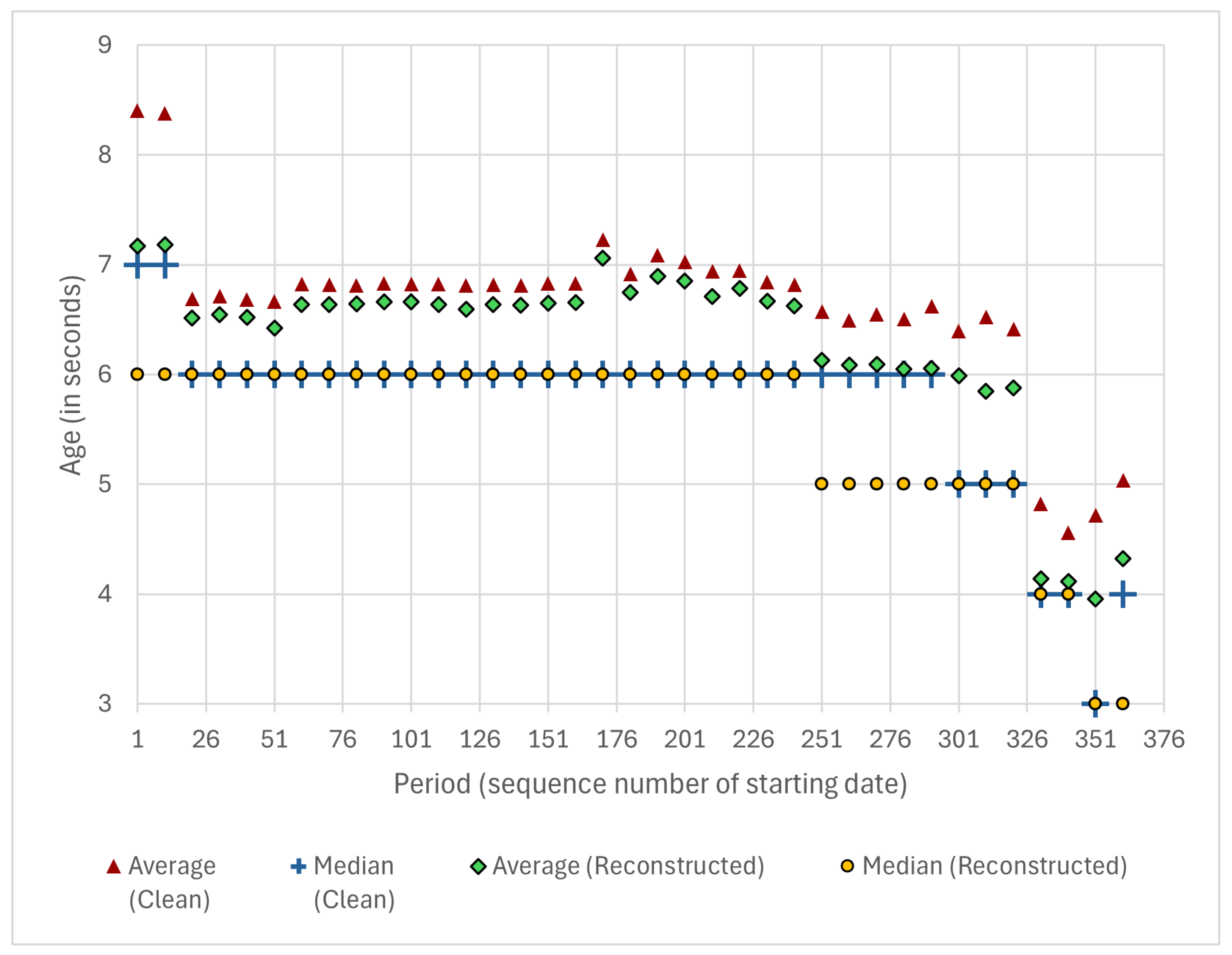
4.1.2. Ratio and Age of Tracked Trips
- What is the age (the elapsed time between the timestamps of recording and fetching) of the collected vehicle positions?
- Could the age be enhanced by increasing the frequency of the requests over the periods?
- Average (Clean)—This series contains the average age of the clean dataset per service date. The period P1 had an average of s, while periods P2 and P3 had an average of s; finally, period P4 had an average of s. Consequently, the age of the cleaned dataset decreased by increasing the query frequency through the periods.
- Median (Clean)—The pattern that can be realized in the medians is similar to the averages’ one: in period P1, we could only reach a median of 7, but period P3 could reach a median of 3, which guarantees extremely accurate and fresh data.
- Average (Reconstructed)—An interesting feature can be detected in the dataset: the average delta decreases if the reconstruction stage is applied. As a speculation, BKK’s system determines the analyzed properties such as stop sequences and stop ID more accurately if the vehicle positions are fresh; moreover, vehicles that do not sign off from their trips generate greater deltas while standing in the terminuses or in depots.
- Median (Reconstructed)—The clean and reconstructed medians meet each other. The median was always less than the average except for period P4.
4.1.3. Validating the Raw and Cleaned Scheduled Trips
- Applying the strong validation before performing the reconstruction method on the tracked trips, we can detect only 29 days providing more than valid trips, while the median of the non-tracked trips’ ratio is . Finally, the median of the invalid trips’ ratio is .
- Applying the strong validation after performing the reconstruction method on the tracked trips, the median of the valid trips’ ratio is , while the median of the invalid trips’ ratio is .
- Applying the weak validation after performing the reconstruction method on the tracked trips, accepting trips annotated with the labels HEAD_1, TAIL_1, and GAP_1 increases the median of the valid trips’ ratio to , decreasing the median of the invalid trips’ ratio to .
4.2. Interactive Visualization of the Dataset
- Layer map covers Hungary to support suburban routes leaving the boundary of Budapest.
- Layer shapes contains those shapes that had scheduled trips for the selected time period for the given routes.
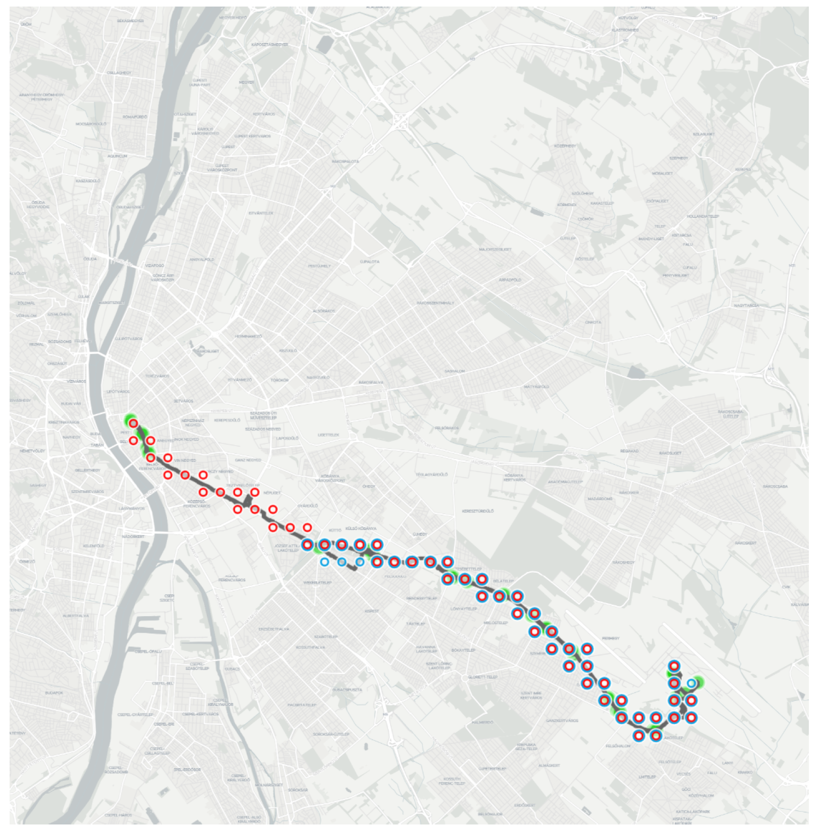
- Layer stops contains markers for the available stops of the displayed shapes.
- Layer vehicles contains markers for those positions that have recorded vehicles in the GTFS-RT feed Vehicle Positions.
4.2.1. Layer Shapes
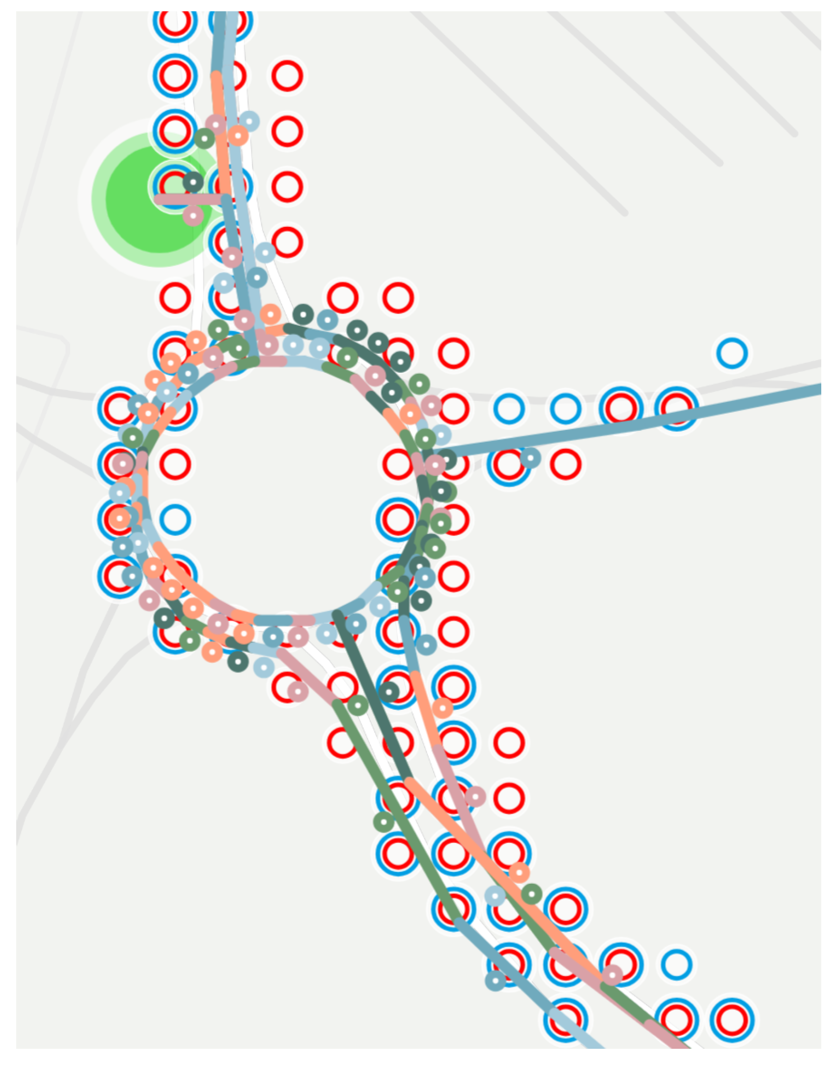
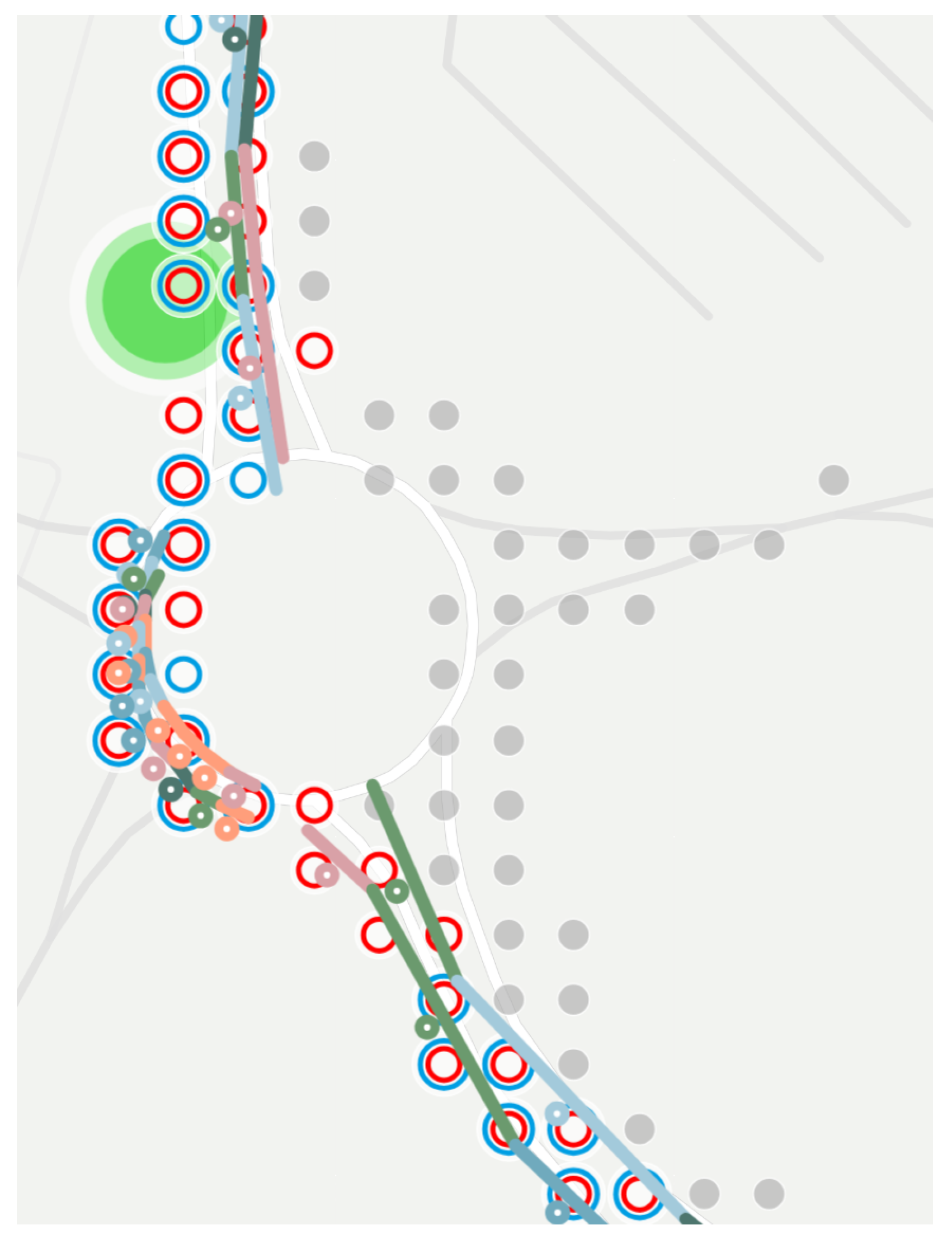
- Segment , belonging to direction 0 of a route usually appears as segment , describing the same route in direction 1. If the streets are narrow, this representation is the most suitable for processing the data and visualizing the routes.
- Parallel shapes—which are heading in the same direction on the same street—are built from different waypoints, resulting in a disjunct but overlapping set of edges. For creating a network (e.g., for visualizing traffic-related congestion, delay times, and throughput), a post-processing algorithm would be required to simplify the shapes and rebuild them from common vertices and shared edges.
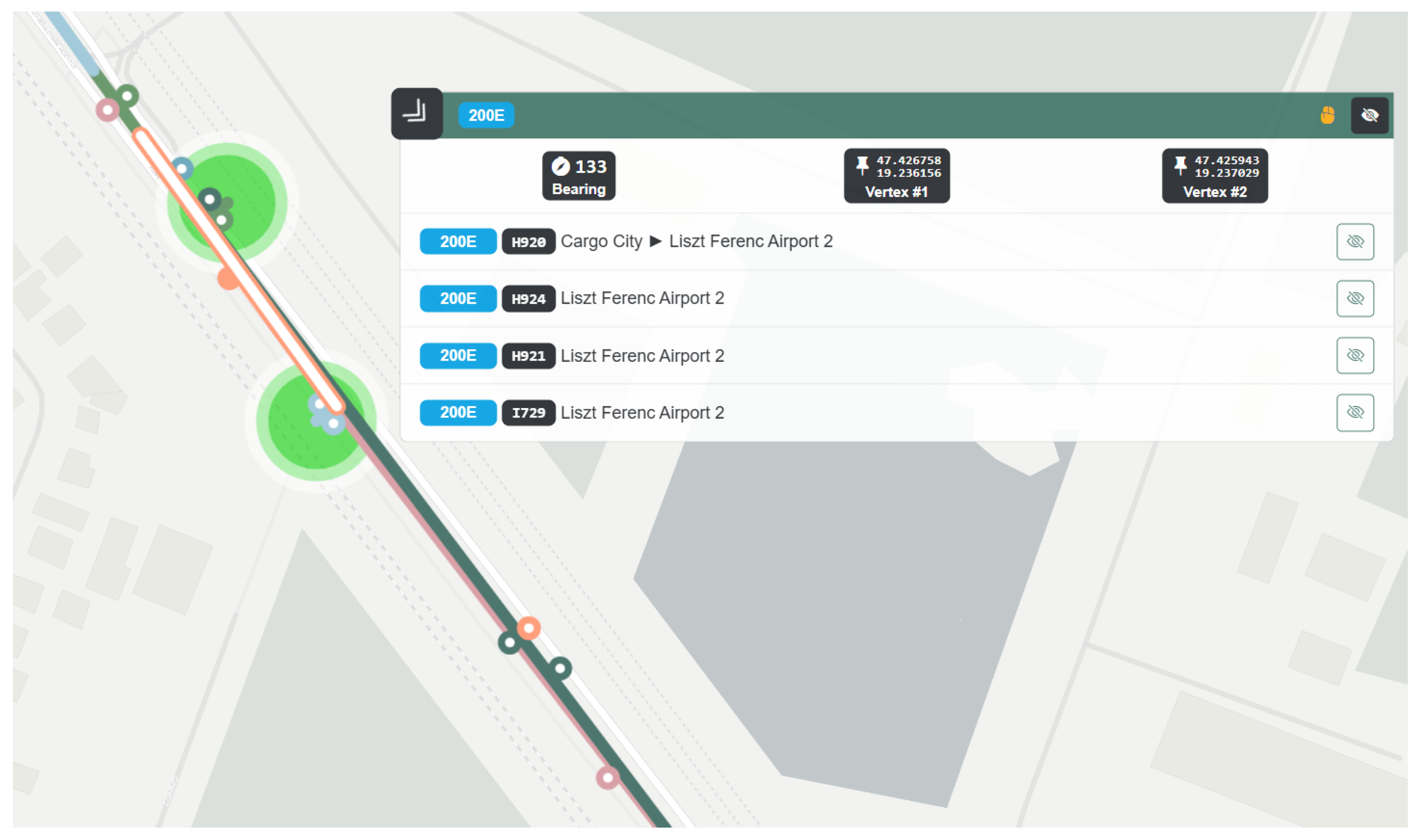
- Waypoints are added with precision errors; this feature can be recognized by having local knowledge, but the visualization of overlapping edges can simplify their detection. For example, the “Liszt Ferenc Airport 2” is served by the already visualized routes 100E and 200E; the former one is an express route from the downtown, and the second one provides regular service from the Eastern districts of Budapest. Their shapes provide many anomalies, such as crossing each other and being misplaced on the wrong side of the expressway around the terminals. This leads to placing vertices further away from their desired location than the real distance of them in those sections where the 100E route uses a rapid highway while the 200E route uses the parallel street. Thus, fixing these shapes by applying a constant threshold and merging the parallel edges would be insufficient.
4.2.2. Layer Vehicles
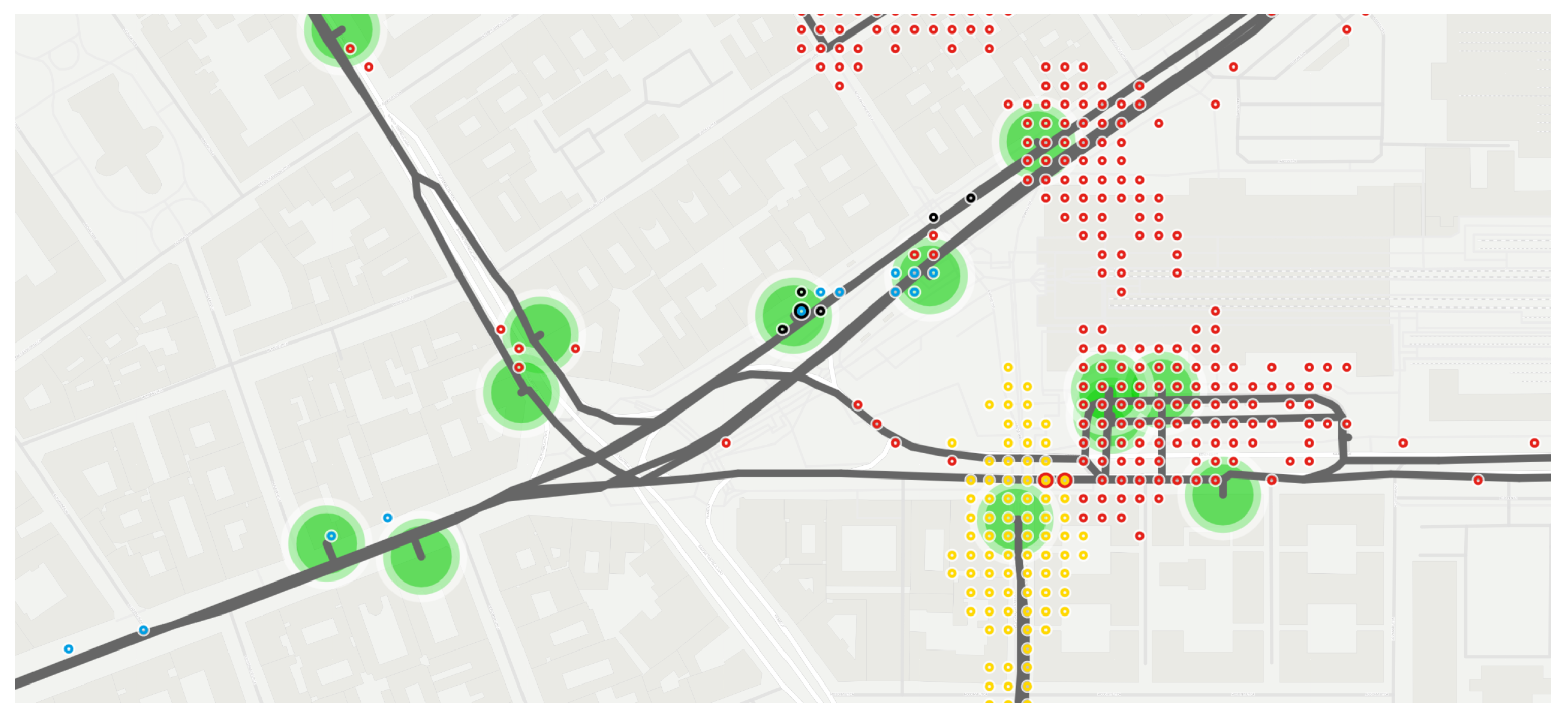
- Tracked positions can be inaccurate, especially when vehicles are staying at stops and surrounded by buildings. As our hypothesis suggests, this feature can also lead to miscalculations of the environment and result in the representation of trip logs. This feature was detected near the terminus “Liszt Ferenc Airport 2”, where the vehicles just under the facade of the terminal building and an elevated road are also partially covered (see Figure 4).
- Misaligned waypoints and edges can be detected by displaying the vehicles serving the corresponding trips. A reconstruction algorithm could adjust the shapes dynamically by checking the vehicle positions.
- For future visualizations, the throughput, delays, and all the features can be visualized for individual directions using the bearing (direction) filters. Busy junctions do not necessarily have the same features for all the crossing directions.
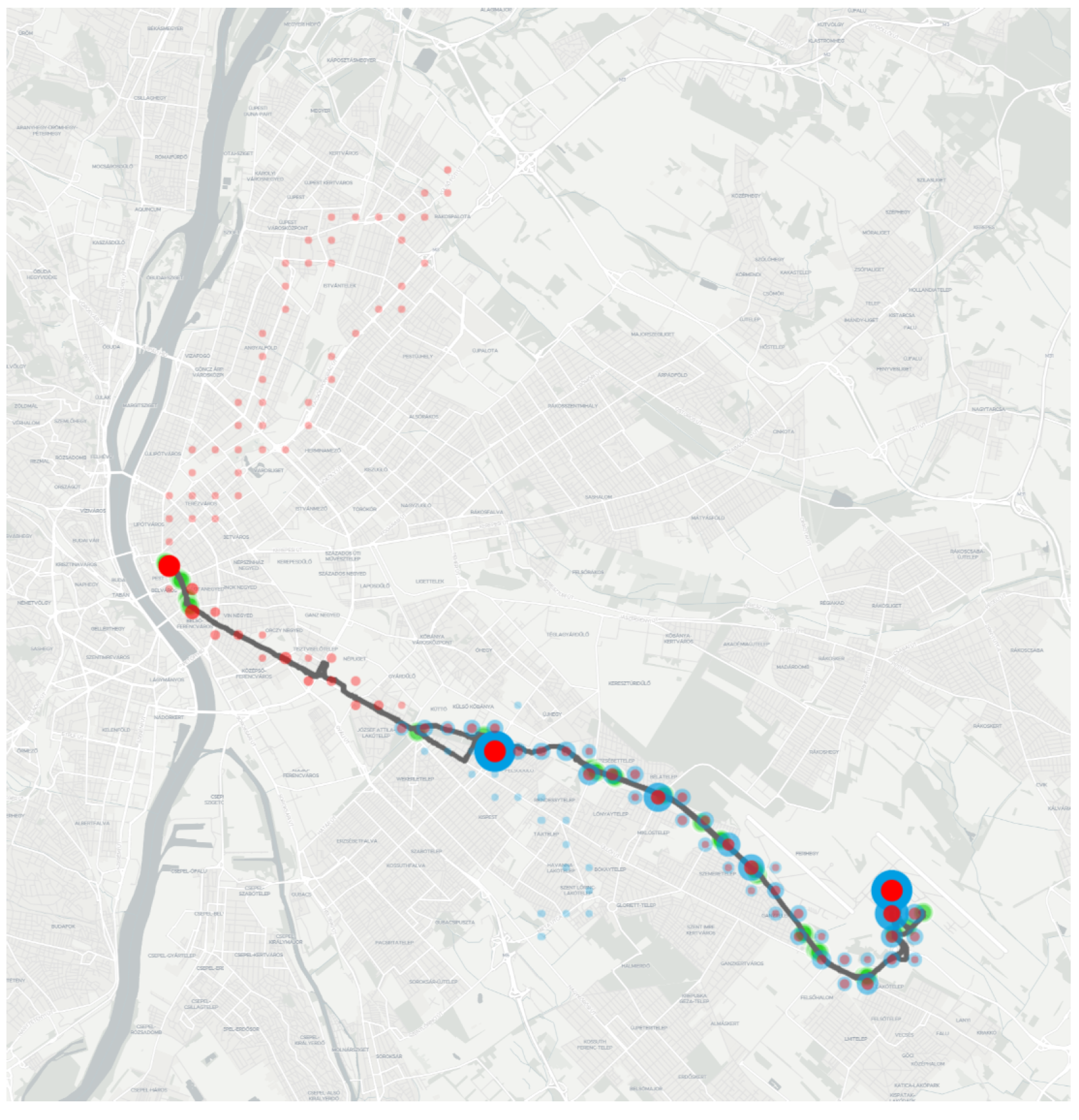
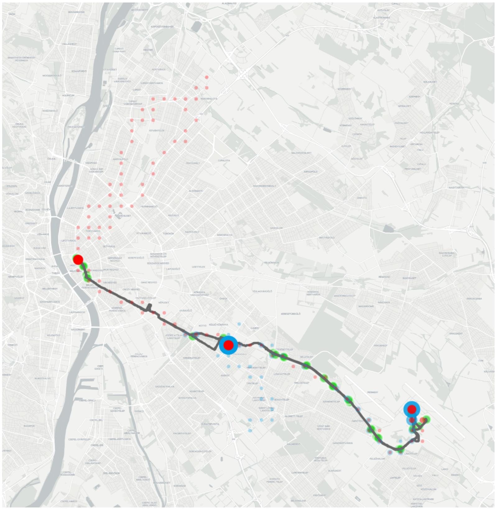
- Colors mode displays each position as a set of Circle markers aligned to the middle of the covered area. By default, the GTFS routes’ official colors are being used; however, users can differentiate each route from one another, providing an opportunity to distinguish different kinds of services such as trams, trolleybuses, and buses. This feature was used in Figure 4 for the routes 100E and 200E.
- Heatmap mode displays the tracked positions as a heatmap; the opacity and the size of a marker are greater if more recorded vehicles are part of it in the displayed area. Similar to the previous mode, each color has its own component, making their parallel visualization possible. This feature is used in Section 4.2.3 to visualize the amount of noise around the terminuses.
- Sublayer vehicles-filtered—contains the filtered set of tracked positions;
- Sublayer vehicles-fixed—contains the reconstructed set of tracked positions;
- Sublayer vehicles-diff—contains those vehicle positions that were classified as noise by our validating and reconstruction algorithm.
4.2.3. Analysis
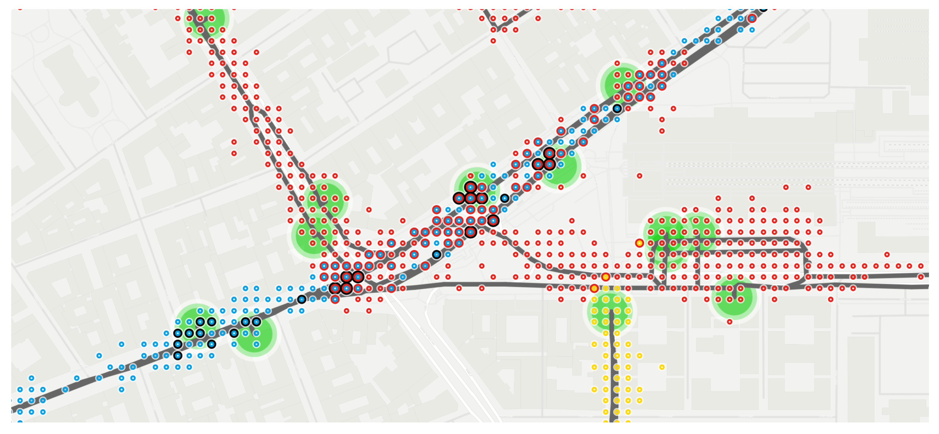
- Many noises were recorded around the terminuses, as Figure 12 shows.
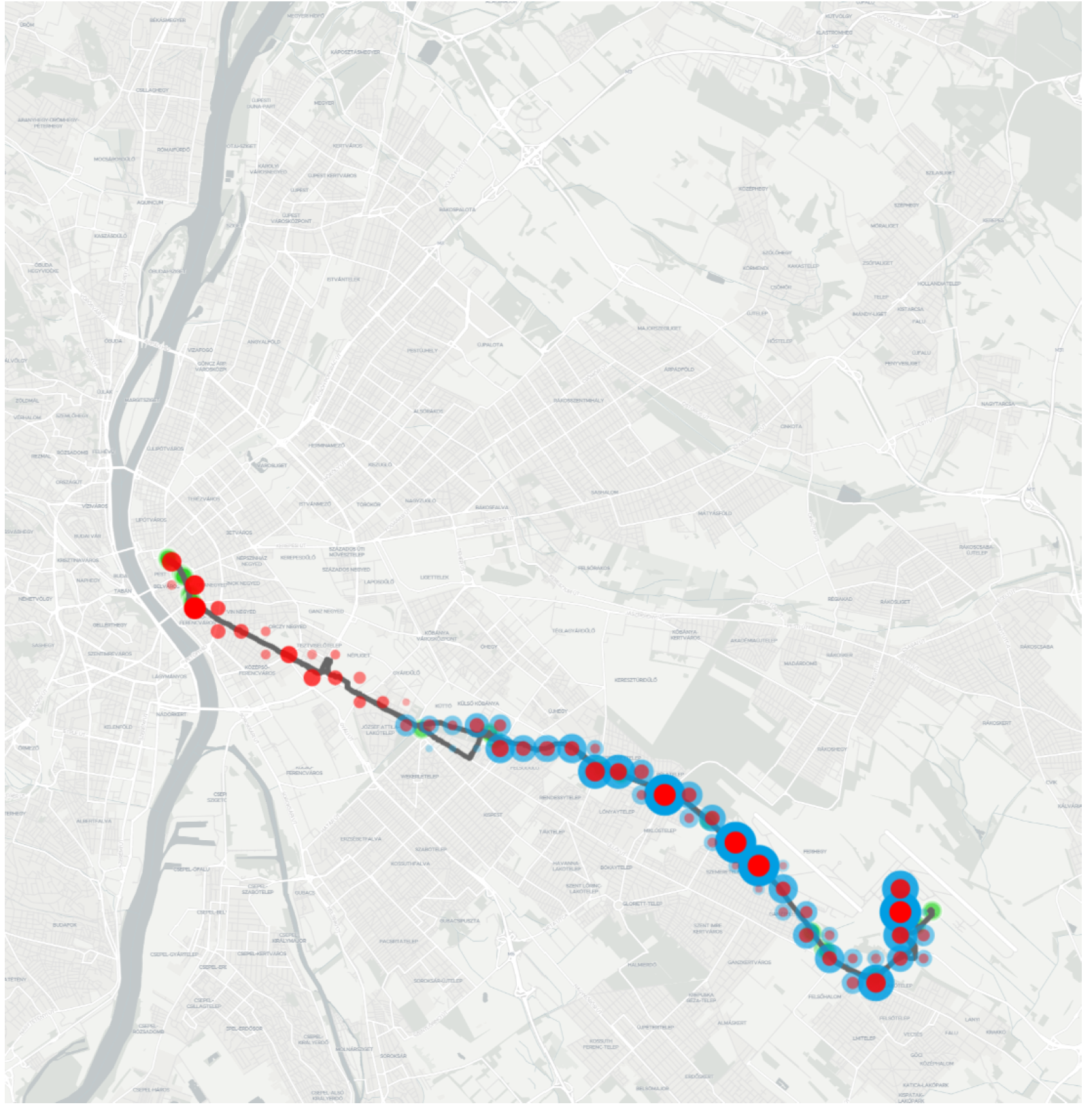
- As Figure 11 shows, various locations were tracked in the Northern and Southern districts. The vehicles left the shapes belonging to routes 100E and 200E. Manually checking the extra positions, an interesting exploration can be made: the red markers head to the depot of the company providing the service for route 100E, while the blue markers head to the depot of the company providing the service for route 200E.
5. Conclusions
Author Contributions
Funding
Institutional Review Board Statement
Informed Consent Statement
Data Availability Statement
Acknowledgments
Conflicts of Interest
Abbreviations
| API | Application Programming Interface |
| BKK | The Centre for Budapest Transport |
| CSV | Comma-separated values |
| GPS | Global Positioning System |
| GTFS | General Transit Feed Specification |
| GTFS-RT | General Transit Feed Specification Realtime |
| JSON | JavaScript Object Notation |
| MÁV | MÁV-START Railway Passenger Transport Company |
| MÁV-HÉV | MÁV-HÉV Suburban Railway Company |
| OSM | OpenStreetMap |
| PB | Protocol Buffers |
References
- Gonzalez, M.C.; Hidalgo, C.A.; Barabasi, A.L. Understanding individual human mobility patterns. Nature 2008, 453, 779–782. [Google Scholar] [CrossRef]
- Walker, R.A. A theory of suburbanization: Capitalism and the construction of urban space in the United States. In Urbanization and Urban Planning in Capitalist Society; Routledge: Abingdon-on-Thames, UK, 2018; pp. 383–429. [Google Scholar]
- Pieretti, G. Suburbanization. In Encyclopedia of Quality of Life and Well-Being Research; Springer: Berlin/Heidelberg, Germany, 2024; pp. 7009–7011. [Google Scholar] [CrossRef]
- Buchanan, M. The benefits of public transport. Nat. Phys. 2019, 15, 876. [Google Scholar] [CrossRef]
- Gase, L.N.; Kuo, T.; Teutsch, S.; Fielding, J.E. Estimating the costs and benefits of providing free public transit passes to students in Los Angeles County: Lessons learned in applying a health lens to decision-making. Int. J. Environ. Res. Public Health 2014, 11, 11384–11397. [Google Scholar] [CrossRef]
- Zhao, F.; Fashola, O.I.; Olarewaju, T.I.; Onwumere, I. Smart city research: A holistic and state-of-the-art literature review. Cities 2021, 119, 103406. [Google Scholar] [CrossRef]
- Camero, A.; Alba, E. Smart City and information technology: A review. Cities 2019, 93, 84–94. [Google Scholar] [CrossRef]
- Meijer, A.; Bolívar, M.P.R. Governing the smart city: A review of the literature on smart urban governance. Int. Rev. Adm. Sci. 2016, 82, 392–408. [Google Scholar] [CrossRef]
- Besenczi, R.; Bátfai, N.; Jeszenszky, P.; Major, R.; Monori, F.; Ispány, M. Large-scale simulation of traffic flow using Markov model. PLoS ONE 2021, 16, e0246062. [Google Scholar] [CrossRef]
- Trencher, G. Towards the smart city 2.0: Empirical evidence of using smartness as a tool for tackling social challenges. Technol. Forecast. Soc. Change 2019, 142, 117–128. [Google Scholar] [CrossRef]
- Bris, A.; Cabolis, C.; Lanvin, B.; Milner, W.; Madureira, O.; Caballero, J.; Zargari, M.; Sharma, C.; Grimm, F.; Tozer, A. Smart City Index Report 2024; Technical Report; IMD World Competitiveness Center: Lausanne, Switzerland, 2024. [Google Scholar]
- Zini, A.; Roberto, R.; Corrias, P.; Felici, B.; Noussan, M. Accessibility Measures to Evaluate Public Transport Competitiveness: The Case of Rome and Turin. Smart Cities 2024, 7, 3334–3354. [Google Scholar] [CrossRef]
- McHugh, B. Pioneering open data standards: The GTFS Story. In Beyond Transparency: Open Data and the Future of Civic Innovation; Code for America Press: Oakland, CA, USA, 2013; pp. 125–135. [Google Scholar]
- Zhou, J.Q.; Jackson, J.; Stravitz, P.; Barlow, G.J.; Koonce, P. Addressing Data Latency in GTFS (General Transit Feed Specification) Realtime to Improve Transit Signal Priority. Transp. Res. Rec. 2024, 2679, 1329–1341. [Google Scholar] [CrossRef]
- Newmark, G.L. Assessing GTFS Accuracy [Research Brief]; Technical Report; San Jose State University. College of Business, Mineta Transportation Institute: San Jose, CA, USA, 2024. [Google Scholar] [CrossRef]
- Kunz, N.; Gao, H.O. Global Geolocated Realtime Data of Interfleet Urban Transit Bus Idling. arXiv 2024, arXiv:2403.03489. [Google Scholar] [CrossRef]
- Wessel, N.; Allen, J.; Farber, S. Constructing a routable retrospective transit timetable from a real-time vehicle location feed and GTFS. J. Transp. Geogr. 2017, 62, 92–97. [Google Scholar] [CrossRef]
- Bok, J.; Kwon, Y. Comparable Measures of Accessibility to Public Transport Using the General Transit Feed Specification. Sustainability 2016, 8, 224. [Google Scholar] [CrossRef]
- Hadas, Y. Assessing public transport systems connectivity based on Google Transit data. J. Transp. Geogr. 2013, 33, 105–116. [Google Scholar] [CrossRef]
- Braga, C.K.V.; Loureiro, C.F.G.; Pereira, R.H. Evaluating the impact of public transport travel time inaccuracy and variability on socio-spatial inequalities in accessibility. J. Transp. Geogr. 2023, 109, 103590. [Google Scholar] [CrossRef]
- Vuurstaek, J.; Cich, G.; Knapen, L.; Ectors, W.; Yasar, A.U.H.; Bellemans, T.; Janssens, D. GTFS bus stop mapping to the OSM network. Future Gener. Comput. Syst. 2020, 110, 393–406. [Google Scholar] [CrossRef]
- Kocsis, G.; Varga, I. gtfs2net: Extraction of General Transit Feed Specification Data Sets to Abstract Networks and Their Analysis. Big Data 2025, 13, 30–41. [Google Scholar] [CrossRef] [PubMed]
- Vágner, A. Route planning on GTFS using Neo4j. Ann. Math. Informaticae 2021, 54, 163–179. [Google Scholar] [CrossRef]
- Alzaidi, M.; Vágner, A. Application-Based Benchmarking on Redis and MongoDB for Trip Planning using GTFS Data. TEM J. Technol. Educ. Manag. Inform. 2023, 12, 2583–2592. [Google Scholar] [CrossRef]
- Alzaidi, M.; Vágner, A. Trip Timing Algorithm for GTFS data With Redis Model to Improve the Performance. J. Theor. Appl. Inf. Technol. 2023, 11, 260–268. [Google Scholar] [CrossRef]
- Fayyaz S, S.K.; Liu, X.C.; Zhang, G. An efficient General Transit Feed Specification (GTFS) enabled algorithm for dynamic transit accessibility analysis. PLoS ONE 2017, 12, e0185333. [Google Scholar] [CrossRef] [PubMed]
- Chaves-Fraga, D.; Priyatna, F.; Cimmino Arriaga, A.; Toledo, J.; Ruckhaus, E.; Corcho, O. GTFS-Madrid-Bench: A Benchmark for Virtual Knowledge Graph Access in the Transport Domain. J. Web Semant. 2020, 65, 100596. [Google Scholar] [CrossRef]
- Devunuri, S.; Lehe, L. A Survey of Errors in GTFS Static Feeds from the United States. Findings 2024. [Google Scholar] [CrossRef]
- Kunama, N.; Worapan, M.; Phithakkitnukoon, S.; Demissie, M. GTFS-Viz: Tool for preprocessing and visualizing GTFS data. In Proceedings of the 2017 ACM International Joint Conference on Pervasive and Ubiquitous Computing and Proceedings of the 2017 ACM International Symposium on Wearable Computers (UbiComp ’17), Maui, HI, USA, 11–15 September 2017; pp. 388–396. [Google Scholar] [CrossRef]
- Prommaharaj, P.; Phithakkitnukoon, S.; Demissie, M.G.; Kattan, L.; Ratti, C. Visualizing public transit system operation with GTFS data: A case study of Calgary, Canada. Heliyon 2020, 6, e03729. [Google Scholar] [CrossRef]
- Para, S.; Wirotsasithon, T.; Jundee, T.; Demissie, M.G.; Sekimoto, Y.; Biljecki, F.; Phithakkitnukoon, S. G2Viz: An online tool for visualizing and analyzing a public transit system from GTFS data. Public Transp. 2024, 16, 893–928. [Google Scholar] [CrossRef]
- Kocsis, G.; Varga, I. Extracting Mass Transportation Networks from General Transit Feed Specification Datasets. In Proceedings of the 7th International Conference on Complexity, Future Information Systems and Risk (COMPLEXIS 2022), Online, 22–23 April 2022; pp. 85–91. [Google Scholar] [CrossRef]
- Wessel, N.; Widener, M.J. Discovering the space–time dimensions of schedule padding and delay from GTFS and real-time transit data. J. Geogr. Syst. 2017, 19, 93–107. [Google Scholar] [CrossRef]
- Aemmer, Z.; Ranjbari, A.; MacKenzie, D. Measurement and classification of transit delays using GTFS-RT data. Public Transp. 2022, 14, 263–285. [Google Scholar] [CrossRef]
- Xian, T.; Moylan, E.; Nelson, J. Evidence from GTFS-R That Bus Priority Lanes Reduce Marginal Delay; Working Paper; School of Civil Engineering, The University of Sydney: Camperdown, Australia, 2022. [Google Scholar]
- Xian, T.; Chin, T.K.; Marks, B.; Nelson, J.; Moylan, E. Bus arrival and departure time updates in the Greater Sydney Area. Sci. Data 2024, 11, 1034. [Google Scholar] [CrossRef]
- Devunuri, S.; Qiam, S.; Lehe, L.J. ChatGPT for GTFS: Benchmarking LLMs on GTFS semantics… and retrieval. Public Transp. 2024, 16, 333–357. [Google Scholar] [CrossRef]
- BKK. Travel Options. Available online: https://bkk.hu/en/travel-information/travel-options-in-budapest/ (accessed on 21 November 2024).
- Khademi-Vidra, A.; Nemecz, G.; Bakos, I.M. Satisfaction measurement in the sustainable public transport of Budapest. Transp. Res. Interdiscip. Perspect. 2024, 23, 100989. [Google Scholar] [CrossRef]


| ID | Start Date | End Date | Vehicle Positions | Trip Updates | Service Alerts |
|---|---|---|---|---|---|
| P1 | 1 September 2023 | 17 September 2023 | 30 | — | — |
| P2 | 18 September 2023 | 3 May 2024 | 15 | — | — |
| P3 | 4 May 2024 | 20 July 2024 | 15 | — | — |
| P4 | 21 July 2024 | 31 August 2024 | 5 | 600 | 600 |
| Range (m) | Strongly Valid Trips | Weakly Valid Trips | ||||
|---|---|---|---|---|---|---|
| 0–5 | 31,087,151 | 4,892,666 | 734,253 | 1,585,362 | 1,380,101 | 184,481 |
| 5–15 | 61,375,162 | 14,279,612 | 3,735,756 | 3,142,669 | 3,675,030 | 800,337 |
| 15–25 | 12,416,218 | 11,746,503 | 4,685,812 | 548,811 | 3,214,766 | 917,629 |
| 25–50 | 20,092,005 | 23,631,221 | 2,425,938 | 937,774 | 6,369,867 | 541,066 |
| 50–100 | 11,244,705 | 23,393,471 | 1,305,257 | 527,450 | 6,587,017 | 397,407 |
| 100–250 | 7,441,194 | 14,792,192 | 1,198,658 | 380,941 | 4,837,538 | 409,886 |
| 250– | 1,575,801 | 5,017,877 | 4,233,268 | 269,683 | 1,999,512 | 1,239,427 |
| Total | 145,232,236 | 97,753,542 | 18,318,942 | 7,392,690 | 28,063,831 | 4,490,233 |
Disclaimer/Publisher’s Note: The statements, opinions and data contained in all publications are solely those of the individual author(s) and contributor(s) and not of MDPI and/or the editor(s). MDPI and/or the editor(s) disclaim responsibility for any injury to people or property resulting from any ideas, methods, instructions or products referred to in the content. |
© 2025 by the authors. Published by MDPI on behalf of the International Society for Photogrammetry and Remote Sensing. Licensee MDPI, Basel, Switzerland. This article is an open access article distributed under the terms and conditions of the Creative Commons Attribution (CC BY) license (https://creativecommons.org/licenses/by/4.0/).
Share and Cite
Tóth, R.; Ispány, M.; Zichar, M. Interactive Visualization for the GTFS and GTFS-RT Data of Budapest. ISPRS Int. J. Geo-Inf. 2025, 14, 245. https://doi.org/10.3390/ijgi14070245
Tóth R, Ispány M, Zichar M. Interactive Visualization for the GTFS and GTFS-RT Data of Budapest. ISPRS International Journal of Geo-Information. 2025; 14(7):245. https://doi.org/10.3390/ijgi14070245
Chicago/Turabian StyleTóth, Róbert, Márton Ispány, and Marianna Zichar. 2025. "Interactive Visualization for the GTFS and GTFS-RT Data of Budapest" ISPRS International Journal of Geo-Information 14, no. 7: 245. https://doi.org/10.3390/ijgi14070245
APA StyleTóth, R., Ispány, M., & Zichar, M. (2025). Interactive Visualization for the GTFS and GTFS-RT Data of Budapest. ISPRS International Journal of Geo-Information, 14(7), 245. https://doi.org/10.3390/ijgi14070245