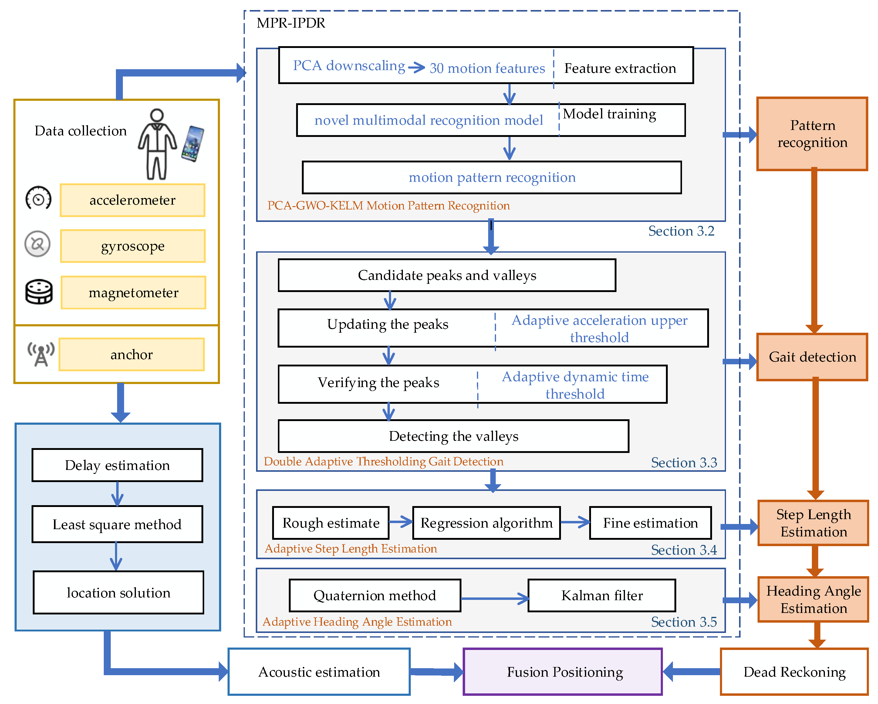
3.2. PCA-GWO-KELM Motion Pattern Recognition
The motion characteristics are extremely related to the complex and diverse target motion postures [
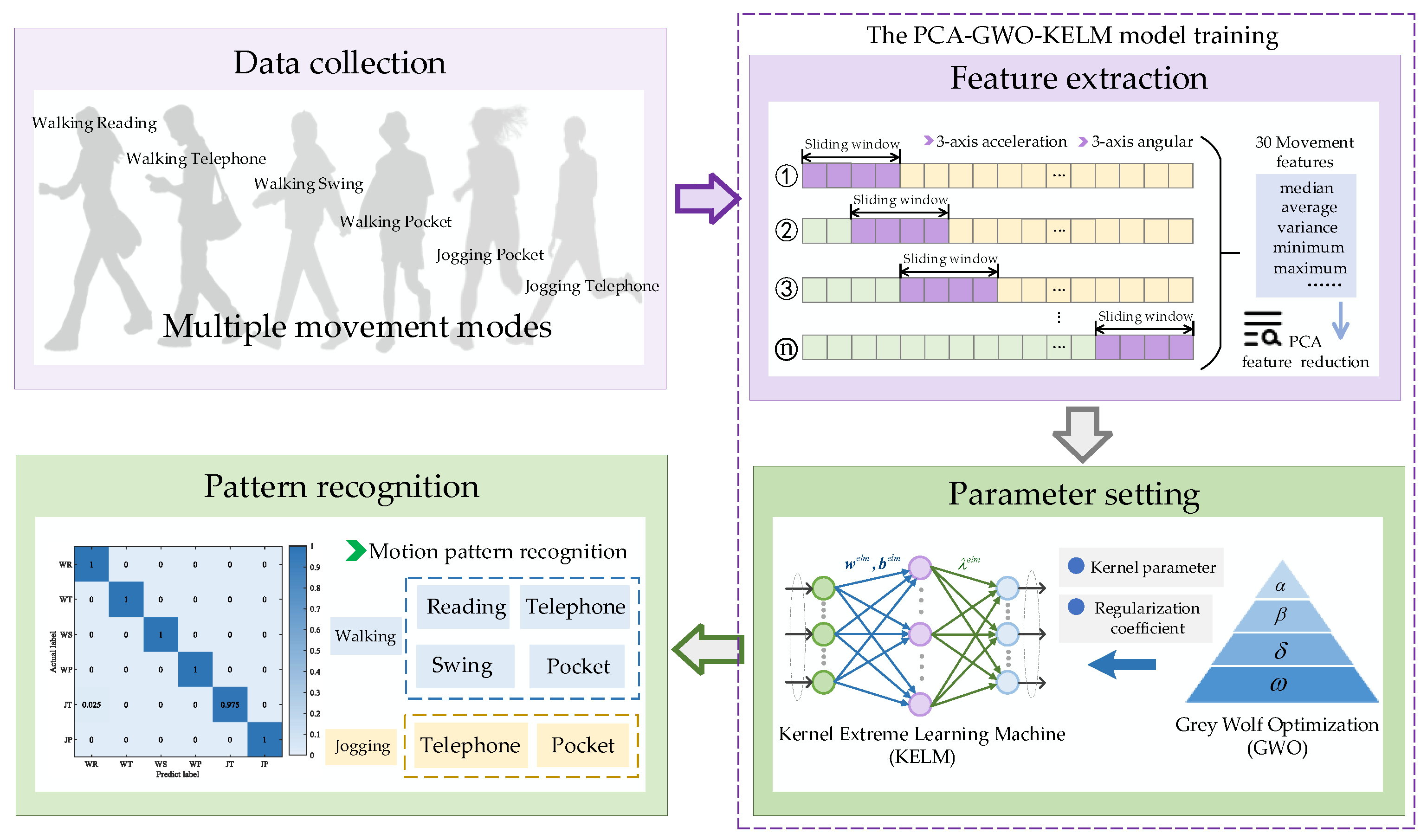
48]. Therefore, how to accurately obtain the target motion characteristics plays a key role in navigation and positioning. The PCA-GWO-KELM motion posture recognition model is proposed in
Figure 2. It mainly includes three stages: data acquisition, feature extraction, and motion mode recognition.
There are differences in acceleration and angular velocity for different motion states during the motion process. This article focuses on collecting three-dimensional motion acceleration and angular velocity data.
Firstly, the original data from accelerators and gyroscopes need to be standardized, which can ensure that all variables have a mean of 0 and a standard deviation of 1, putting them on an equal scale and eliminating the influence of different units. Different features have different importance for motion posture. Sixty-dimensional motion features, including mean, variance, maximum, minimum, energy values, etc., will be obtained from the standardized original accelerators and gyroscope data, which are denoted as . In this paper, we set a data length of 2 s as the sliding window length, and the length of each step is 0.5 s, which results in a 50% data overlap. When the acceleration or angular velocity modulus sequence meets the requirements, the sequence is intercepted, after which the specified window length is slid backward. Repeat the above steps in this way to segment the IMU data to obtain more sample data.
The variable
needs to be standardized by the formula
where
is the
-th sample of the
-th variable,
is the mean of each variable
, and
is the standard deviation.
The covariance matrix
of the standardized data is calculated. The element
of the covariance matrix
is given by
where
is the variance of the
-th variable, and
is the covariance between the
-th and
-th variables. And
is the number of principal components selected.
The next step is to find the eigenvalues and corresponding eigenvectors of the covariance matrix .
This is accomplished by solving the following equation:
The eigenvalues represent the amount of variance explained by the corresponding principal components, and the eigenvectors define the directions of the principal components in the original variable space. Each eigenvector is normalized to have a length of 1, that is, . is the number of variables in the original dataset, and subsequent operations such as calculating the covariance matrix are centered around these variables.
The principal components are ranked according to the magnitudes of their corresponding eigenvalues. Usually, only the first
principal components
are selected, where
is determined based on the amount of variance explained. A common criterion is to choose
such that the cumulative proportion of variance explained by the first
principal component
is given by
where
is the
-th element of the
-th eigenvector
.
The original data are projected onto the selected principal components. For each sample , its projection onto the -dimensional principal component space is expressed as , where for .
This projection transforms the original high-dimensional data into a low-dimensional space, retaining the most important information of the original data. Subsequently, the reduced dimensional motion features are used as the input for PCA-GWO-KELM as the motion postures. In this paper, the input layer dimension of the PCA-GWO-KELM algorithm is the number of features after PCA dimensionality reduction and is set to 10. The hidden layer dimension is 60 and the output layer dimension is 6.
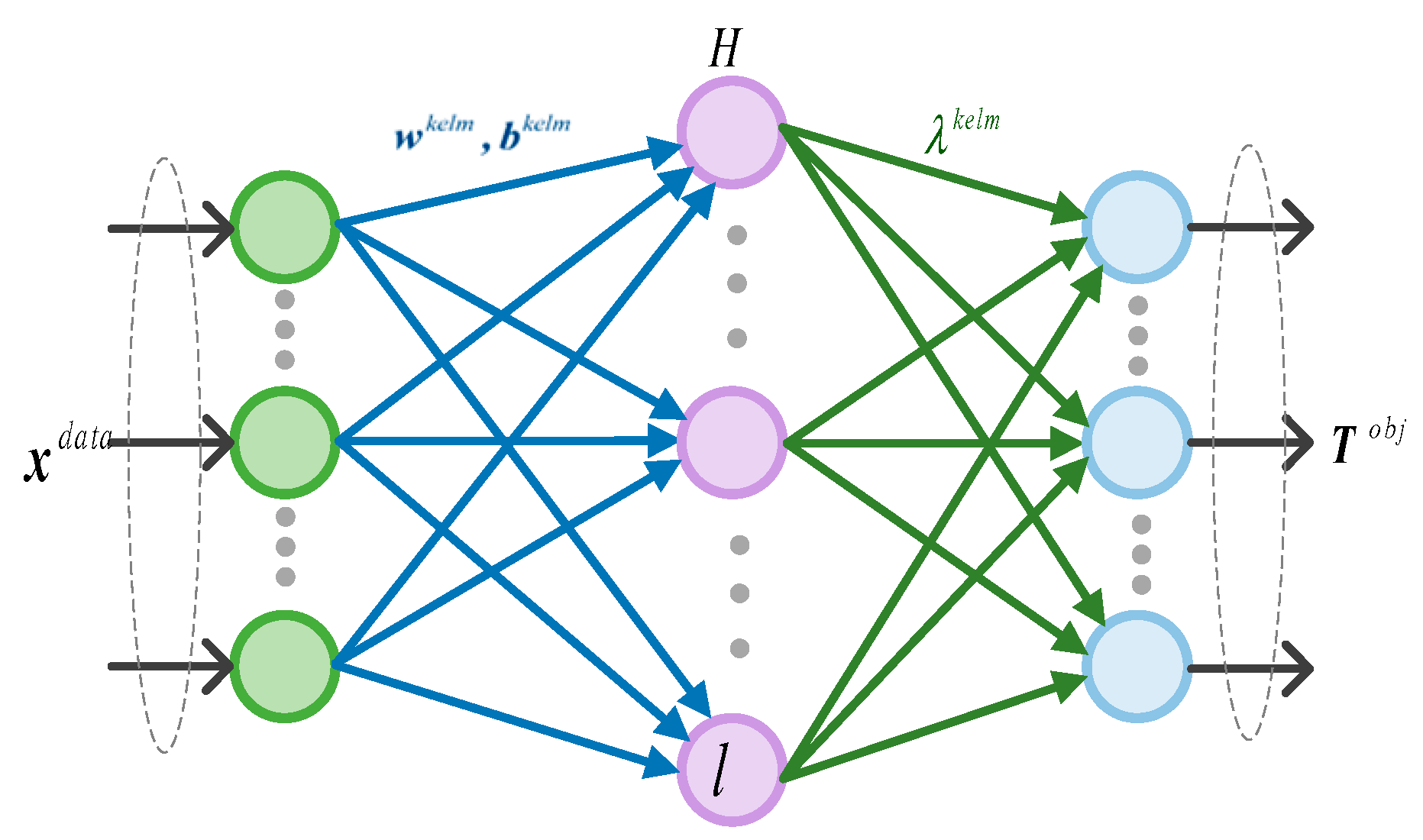
Figure 3 shows kernel extreme learning machine model. Suppose the input dataset
is represented as follows:
The output of the hidden layer
is expressed as
where
represents the activation function of the hidden layer node.
,
are the weight vectors and thresholds connecting the implicit and input layers, respectively, which can be expressed as
where
l denotes the number of nodes in the hidden layer and
s denotes the number of nodes in the input layer.
We design a loss function
. Assuming the target matrix of the training data is denoted by
, and the output of the KELM model can be represented by
, the loss function
is expressed as follows:
where
is the target matrix of the training data,
is the predict output, and
is the connection weight value between the hidden layer and the output layer.
To prevent model overfitting and ensure matrix inverse stability, regularization coefficients
C are added to optimize connection weight
. The update loss function
is as follows:
where
is the L2 regularization penalty.
To achieve the optimization predicted value, it become the optimization question for searching the minimum loss function .
Expanding Equation (10), we obtain
Differentiating Equation (11),
The optimization value of Equation (12) is achieved as below:
Then, the output of KELM is shown as follows:
where
is the kernel function in the KELM model, which is expressed as
From Equation (14), the kernel function parameters and regularization coefficients C are the key factors affecting the prediction performance. The gray wolf optimization (GWO) method is used to optimize the two parameters due to its effectiveness and strong global search ability.
Firstly, a population of N gray wolves is randomly initialized within the search space. The position of each wolf
i is initialized as follows:
where
and
are the lower and upper bounds of the
j-th variable, respectively, and
is a random number uniformly distributed in the range [0, 1].
Each wolf has the individual fitness function and can be expressed as
where
N denotes the number of training samples, and
is the predicted value of the model containing
and
.
The gray wolf algorithm is set with a population size of 50 and a maximum number of iterations of 60. The lower boundary of the wolf pack search space is 1, and the upper boundary is 20. Gray wolves encircle their prey during the hunting process. This behavior is modeled by updating the position of each wolf towards the prey. Wolves
,
,
, and wolf
are identified. Individual gray wolves are positionally updated as follows:
where
,
, and
denote the distances between
,
, and
with the target solution, respectively.
,
, and
denote the positions of
,
, and
at the
th iteration.
denotes the specific position of the current target solution.
Then, the three new candidate positions
,
, and
for each wolf based on the position of wolves
,
, and
is calculated as below:
where
, and
are coefficient vectors.
Finally, the new position of the wolf at the nest iteration is updated as the average of the three candidate positions:
When the search approaches the end, this makes the wolves approach the optimal solution more accurately. This position represents kernel function parameters and regularization coefficients C of the optimized KELM.
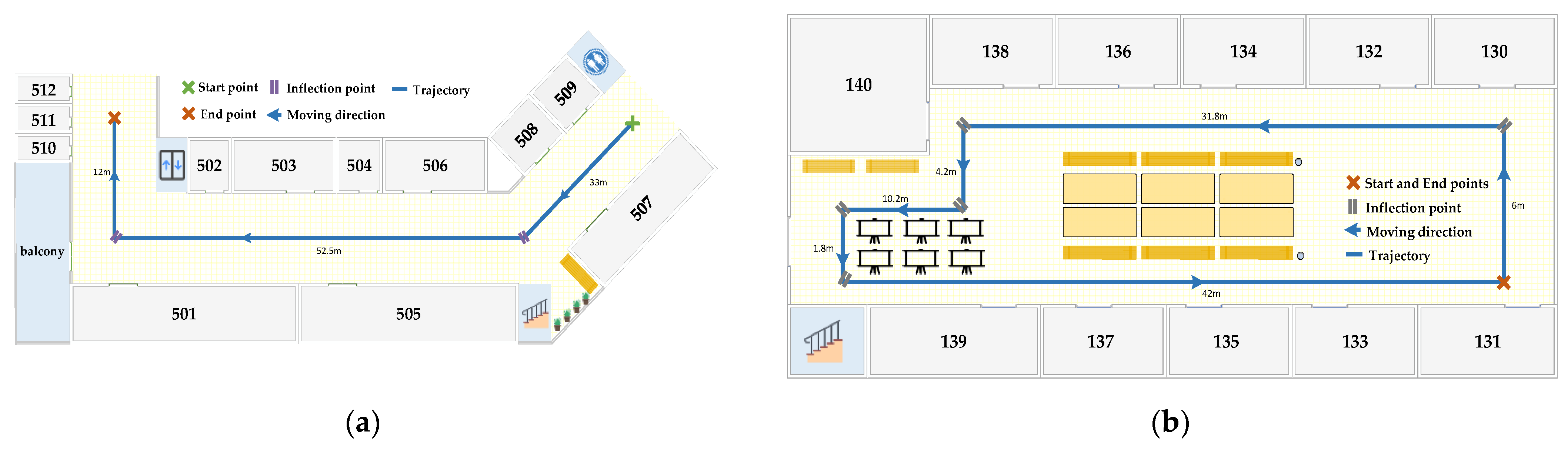
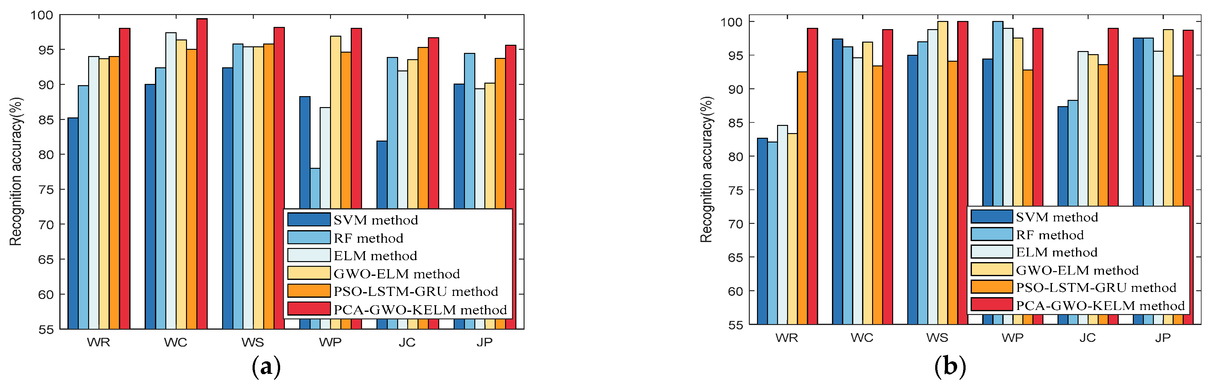
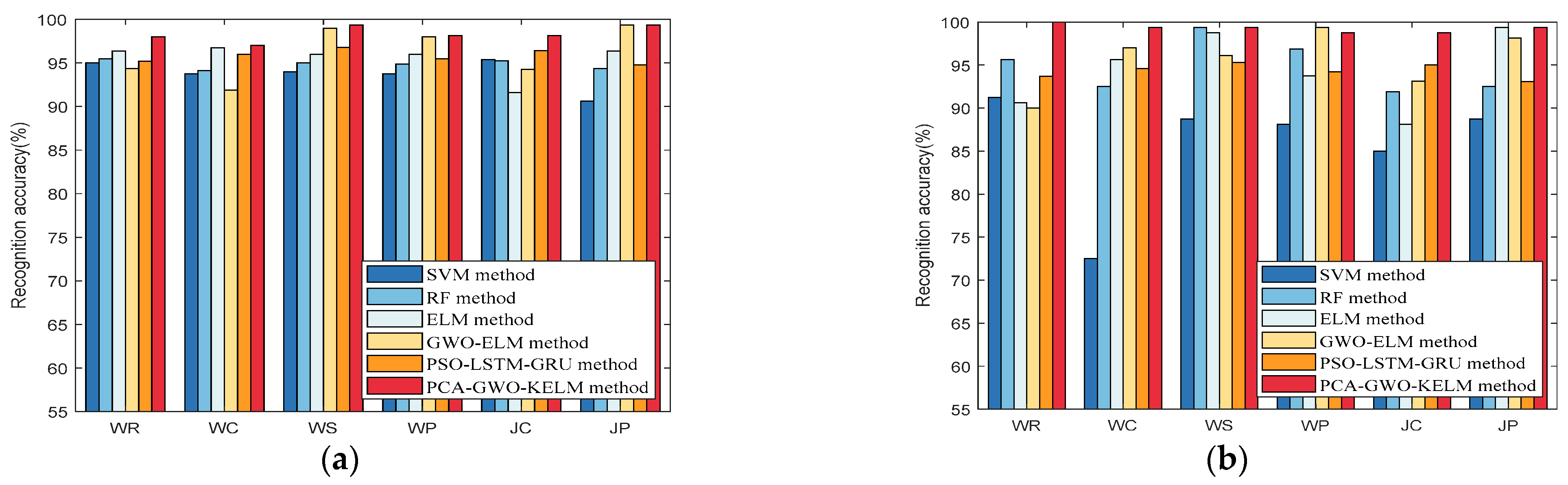
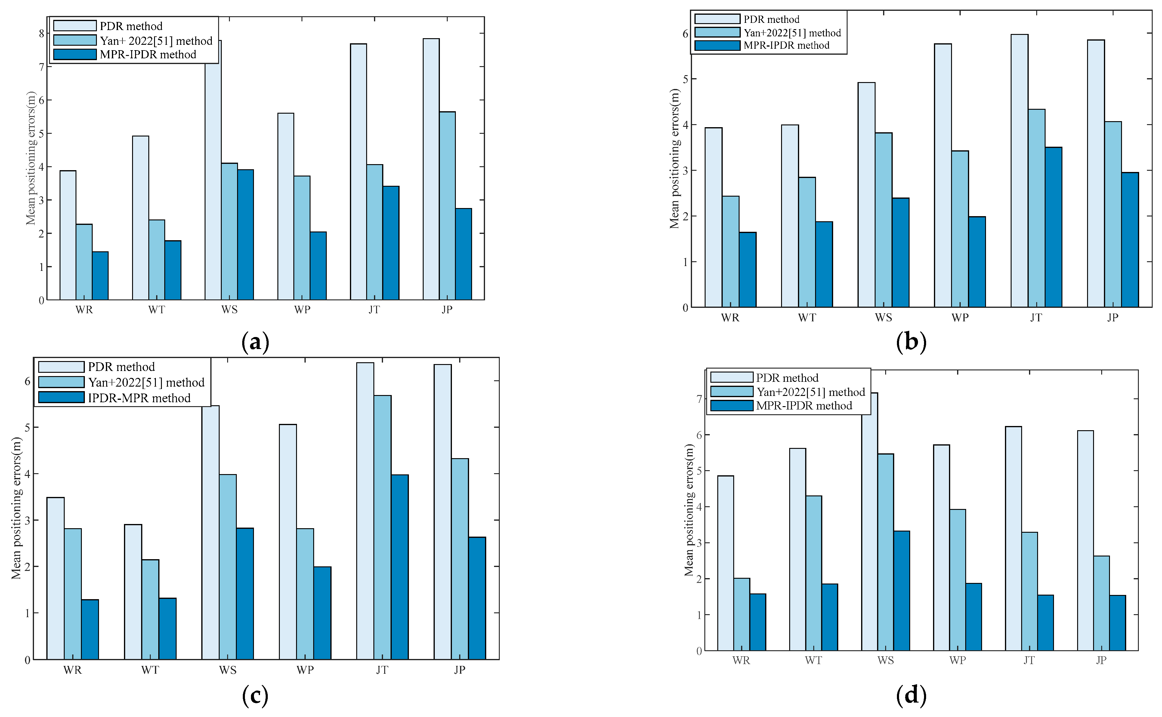
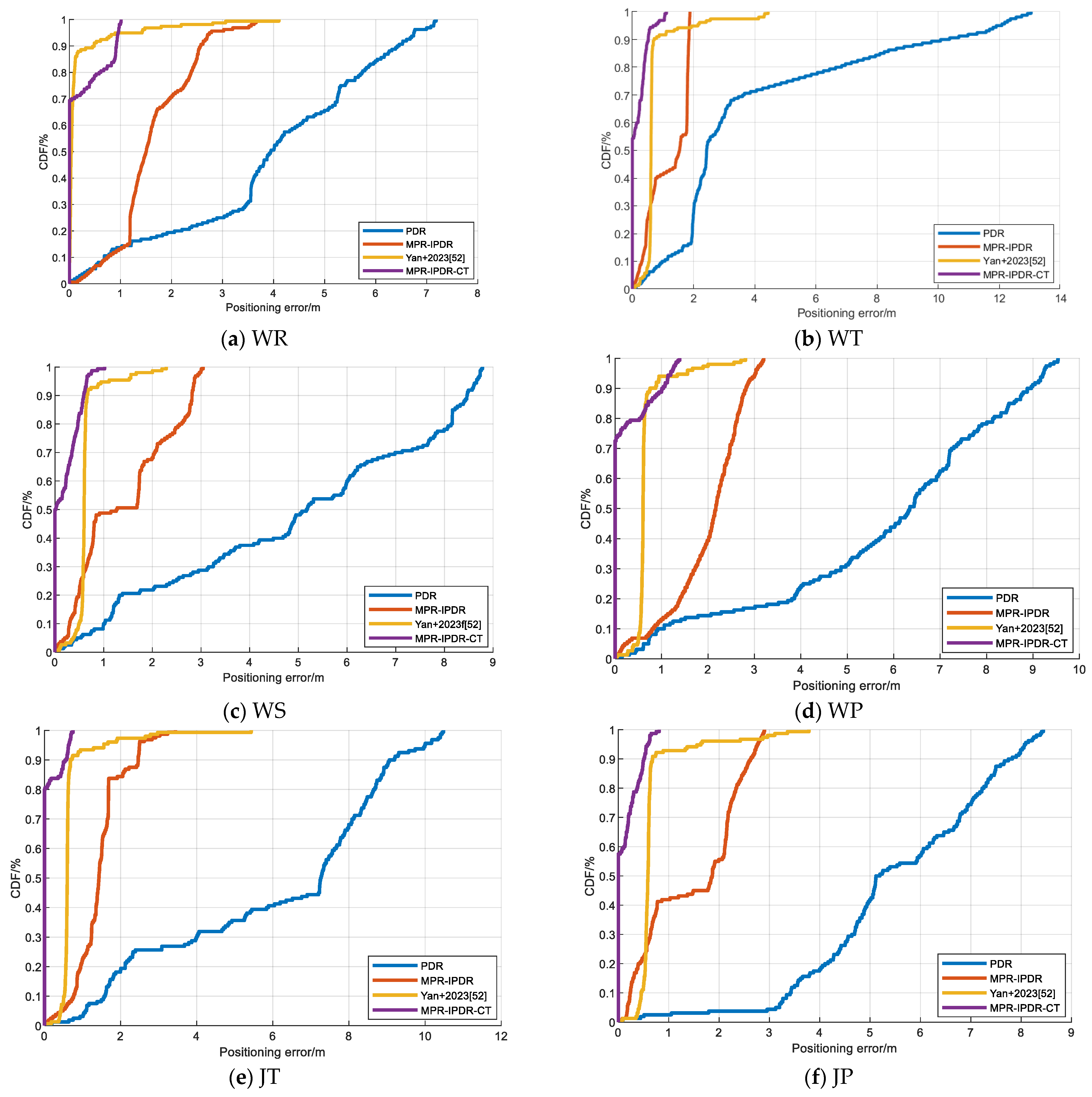
To validate the recognition accuracy of the proposed PCA-GWO-KELM model, experiments have been carried out in two separate experimental paths with six different motion modes, including walking and reading (WR), walking and telephoning (WT), walking and swinging (WS), walking and pocketing (WP), jogging and telephoning (JT), and jogging and pocketing (JP). WR mode refers to when a pedestrian is walking at normal speed with their phone steadily placed in front of their chest. WT mode refers to the situation where a pedestrian is walking at normal speed with their phone held to their ear to answer a call. WS mode refers to the state where a pedestrian’s phone swings at random while walking at normal speed. WP mode refers to the situation where pedestrians place their mobile phones in the side pockets of their pants while walking at normal speed. JT mode refers to the situation where a pedestrian answers a call with their phone held to their ear while running. JP mode refers to the situation where a pedestrian’s phone is placed in the side pocket of their pants while running. The device used in this experiment is Mate60 Pro cell phone. These two planned experimental paths are two indoor straight corridors with a building length of 24 m and 97.2 m, respectively.
Figure 4 presents the accuracy of the proposed PCA-GWO-KELM model in multiple movement model recognition. Results have demonstrated that the accuracy of the motion pattern recognition for WR, WT, WS, WP, JT, and JP modes are, respectively, 100%, 100%, 100%, 100%, 97.50%, and 100% on the 24 m path. And the recognition rates for WR, WT, WS, WP, JT, and JP modes are, respectively, 100%, 99.38%, 98.15%, 100%, 95.68%, and 92.60% on the 97.2 m path. The PCA-GWO-KELM model achieves a high recognition rate of motion pattern under different scenes.
3.3. Double Adaptive Threshold Gait Detection
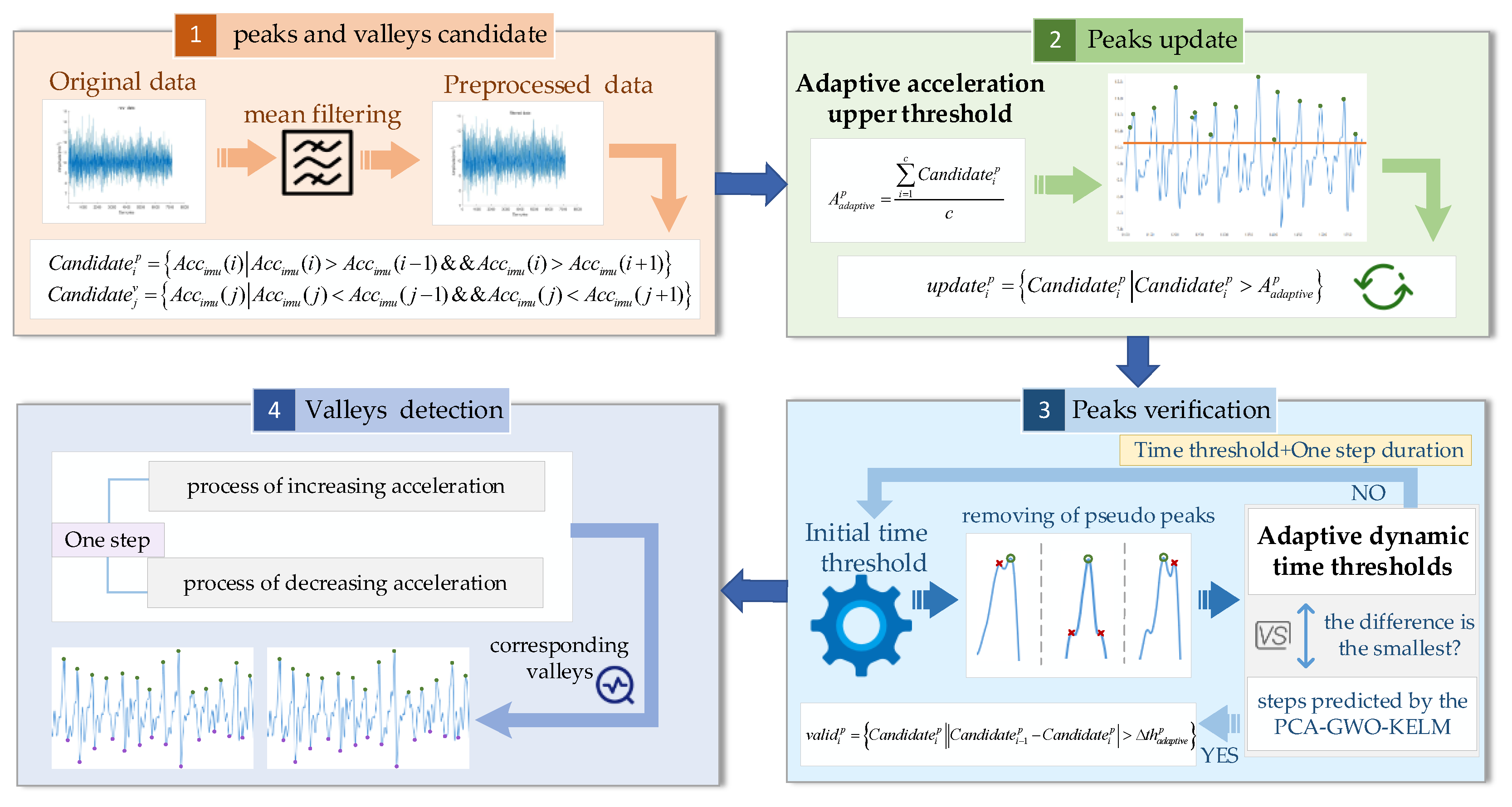
Accurate gait detection can achieve good positioning performance. We propose a double adaptive threshold gait detection method, shown in
Figure 5. The proposed gait detection method includes peak and valley candidates, peak update, peak verification, and valley detection.
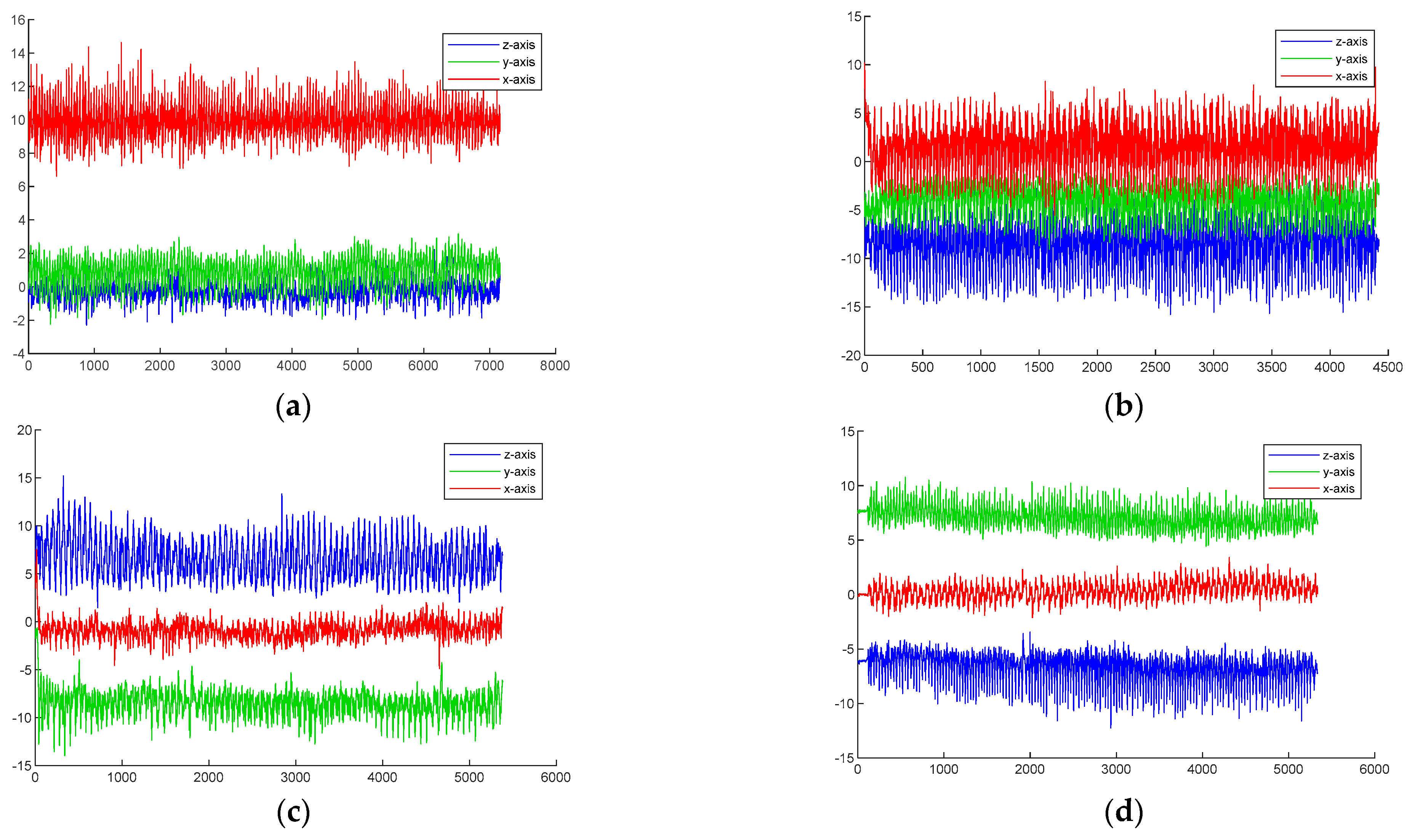
Three-dimensional acceleration under different movements reflects different motion postures.
Figure 6 shows the changes in motion acceleration in reading, phone, swing, and pocket modes. The red line represents the
X-axis acceleration, the green line represents the
Y-axis acceleration, and the blue line represents the
Z-axis acceleration. The results demonstrate that in reading mode and pocket mode, the acceleration changes in the
z-axis and
x-axis directions are more significant. In swing and phone modes, there are significant changes in acceleration in the
x-axis and
y-axis directions. Therefore, there are differences in the motion characteristics of different postures.
In gait detection, candidate peak pre-detection of motion acceleration is first performed using the peak detection method. The peak must be greater than the value of the acceleration before and after it. If a peak is detected, it is considered that the pedestrian has taken a step, and the peak time is recorded, as shown in the following equation:
where
is the set of candidate peaks at sampling point
i.
is the combined acceleration.
To avoid the pseudo peaks, the adaptive acceleration upper threshold is set by taking the average of the forward acceleration within a fixed time period, as shown in Equation (14).
where
is the adaptive acceleration upper threshold, and
c is the number of candidate peaks.
Candidate peaks that are larger than the threshold for adaptive acceleration are saved, and is the set of updated candidate peaks.
The time interval between two adjacent peaks is finite. In this paper, an adaptive dynamic time threshold is set to verify the valid peaks. First, the initial time threshold is set to the time interval of the first step, and the number of prediction steps corresponding to the initial time threshold is recorded. This predicted number of steps then differs from the true number of steps obtained from the PCA-GWO-KELM model. If the difference is minimum at this point, the number of steps corresponding to the initial threshold is output. If the difference is not a minimum, the initial time threshold is doubled, and the algorithm loop continues. The current peak acceleration can be judged valid only if the time interval between two adjacent steps meets the requirements of the following equation.
where
is the set of peaks after verification of the adaptive dynamic time thresholds, and
is an adaptive dynamic time threshold.
The flow of the double adaptive threshold gait detection method is depicted in Algorithm 1.
| Algorithm 1: The double adaptive threshold gait detection method |
| Input: Motion acceleration data. |
| Output: Target steps and peak amplitude. |
| 1: Data preprocessing using mean filtering. |
| 2: Candidate peaks are selected using peak detection by Equation (21). |
| 3: Candidate peaks are counted, and adaptive acceleration upper thresholds are calculated by Equation (22). |
| 4: Update candidate peaks by Equation (23). |
| 5: Set the time interval of the first step to the initial time threshold. |
| 6: for each step do |
| 7: Record the difference between the step number corresponding to the current time threshold and the true step number. |
| 8: if the difference is minimal then |
| 9: Save the step number at this moment. |
| 10: else |
| 11: Double the time threshold. |
| 12: end if |
| 13: Save the value of each peak. |
| 14: end for |
3.6. Multiple Pattern Recognition Positioning
Particle filtering is a recursive Bayesian filtering method for state estimation of dynamic systems, which is suitable for nonlinear and non-Gaussian noise cases. Therefore, we utilized PF combined with PDR and acoustic signals for fusion positioning. The fusion positioning method designed in this paper performs the following steps:
Step 1: Initialize a particle swarm containing particles in the positioning region, each with a weight of 1, and assume that the set of particles at moment t are . The position coordinates of the initial particle set are generated based on the acoustic positioning results.
Step 2: After obtaining the initialized particle set, the position of the particle at time
t + 1 will be updated by Equation (30).
where
and
are the step length and heading angle of the pedestrian at
t + 1, respectively.
is Gaussian noise with zero mean and variance of 1.
Step 3: The acoustic positioning results are used as systematic observations, expressed as follows:
where
and
are the estimated positions for acoustic localization at
t + 1, respectively, and
is the observation noise. The new weight update factor is calculated from the acoustic positioning results as follows:
where
is the covariance matrix of the acoustic estimate.
Step 4: The particles are normalized by Equation (33).
The normalized particles are then resampled. Particles with large weights have a high percentage after resampling, and particles with small weights are discarded. The particles with high weights are replicated multiple times with the total number of particles remaining the same.
Step 5: Finally, fusion positioning estimation is performed. The pedestrian’s position at
t + 1 can be calculated by Equation (34).


 ,
, 


