High-Resolution Global Land Cover Maps and Their Assessment Strategies

Abstract

Global High-Resolution Land Cover Maps (GHRLCs), characterized by spatial resolutions higher than 30 m per pixel, have become essential tools for environmental monitoring, urban planning, and climate modeling. Over the past two decades, new GHRLCs have emerged, offering increasingly detailed and timely representations of Earth’s surface. This review provides an in-depth analysis of recent developments by examining the data sources, methodologies, and validation techniques utilized in 19 global binary and multi-class land cover products. The evolution of GHRLC production techniques is analyzed, starting from the use of singular source input data, such as multi-temporal remotely sensed optical imagery, to the integration of satellite radar and other geospatial data. The article highlights significant advances in data pre-processing and processing, showcasing a shift from classical methods to modern approaches, including machine learning (ML) and deep learning techniques (e.g., neural networks and transformers), and their direct application on powerful cloud-computing platforms. A comprehensive analysis of the temporal dimension of land cover products, where available, is conducted, highlighting a shift from decadal intervals to production intervals of less than a month. This review also addresses the ongoing challenge of land cover legend harmonization, a topic that remains crucial for ensuring consistency and comparability across datasets. Validation remains another critical aspect of GHRLC production. The methods used to assess map accuracy and reliability, including statistical techniques and visual inspections, are briefly discussed. The validation approaches adopted in recent studies are summarized, with an emphasis on their importance in maintaining data integrity and addressing emerging needs, such as the development of common validation datasets. Ultimately, this review aims to provide a comprehensive overview of the current state and future directions of GHRLC production and validation, highlighting the advancements that have shaped this rapidly evolving field.

1. Introduction

Land cover (LC) maps are essential tools for understanding human and natural processes within land systems. They are widely used among a variety of applications, including post-disaster recovery monitoring [1,2], urban planning [3], Sustainable Development Goals (SDGs) monitoring [4], and climate change research [5]. Given the escalating impacts of global climate change and human activities on ecosystems, there is an increasing demand for high-resolution, accurate, and up-to-date LC maps to effectively understand and respond to environmental land changes [6].

The rapid advancement of satellite remote sensing technology, cloud-based processing, and the extensive application of machine learning in remote sensing have enabled the rapid production of LC maps with high temporal and spatial resolutions. Landsat data has drawn significant attention due to its open-access policy, long-term temporal coverage, and 30-m spatial resolution, leading to the development of numerous 30-m resolution global land cover (GLC) maps [7,8,9,10,11,12,13,14,15]. Since 2014, Sentinel satellites have been providing globally consistent optical and SAR data with a spatial resolution of 10–20 m, driving the generation of 10-m resolution GLC products [16], such as ESRI LULC [17], ESA WorldCover [18,19], and Google Dynamic World [20].

However, HRLC maps present varying classification results depending on the data sources and classification methods. Therefore, a comprehensive evaluation and comparison of these maps is crucial to ensuring their reliability across different applications. In recent years, several studies have explored the status, challenges, and trends in LC mapping from various perspectives. They focus on topics like Earth observation data [21,22], deep learning technologies [23,24,25], big data [26], or land-use and land-cover change [27]. While some studies [28,29] provide general overviews of land cover mapping, there remains a lack of a systematic review that thoroughly compares and evaluates the data sources, key technologies, and validation methodologies underlying these datasets.

Given the importance of GHRLC maps for various applications, and the emergence of HRLC products over the past two decades, we aim to provide a comprehensive overview of the current status and future directions of GHRLC production and validation by examining the data sources, methods, and validation techniques used for 19 global binary or multi-class LC products with a spatial resolution of equal and higher than 30 m. On the other hand, considering the critical role of the Amazon biome in the global climate, we also included the MapBiomas, which provides detailed multi-temporal LC data for this region. A comprehensive list of all HRLC products utilized in this study is provided in

Table 1. Overview of HRLC products used in this study.

Dataset Name	Provider	Spatial Resolution (m)	Temporal Resolution	LC Focus
Dynamic World (DW) [20]	World Resources Institute Google	10	Near real-time from 2015-06-27 to present	General (9 classes)
ESRI LULC [17]	Impact Observatory, Microsoft, and Esri	10	Annual (2017–2023)	General (10 classes)
Forest/Non-Forest (FNF) [30]	JAXA-EORC	25	Annual (2007–2010)	Forest (3 classes)
FROM-GLC10 [31]	Tsinghua University	10	2017	General (10 classes)
FROM-GLC30 [7,31,32]	Tsinghua University	30	2010, 2015, 2017	General (10 classes)
Global Forest Cover (GFC) [33]	JRC	10	2020	Forest (1 class)
GHS-BUILT-S R2023A [34]	JRC	10	2018	Built-Up surface proportion (continuous 0–100%)
GHS-BUILT-S1 2016 [35]	JRC	20	2016	Built-Up (2 classes)
Global 30m impervious-surface dynamic dataset (GISD30) [11]	CAS	30	Interval-encoded (per pixel): before 1985, 1985–1990, 1990–1995, 1995–2000, 2000–2005, 2005–2010, 2010–2015, 2015–2020	Built-Up (1 class)
GlobeLand30 (GL30) [8]	NGCC	30	2000, 2010, 2019	General (10 classes)
Global Land Cover Estimation (GLanCE) v001 [10]	BU/EE/ NASA ES/ USGS EROS	30	Annual (2001–2019)	General (7 classes)
Global 30 m land-cover (dynamics monitoring) product with a fine classification system (GLC_FCS30/D)  [13,14]	CAS	30	Every 5 years (1985, 1990, 1995) and Annual (2000–2022)	General (35 classes)
Global Surface Water (GSW) [9])	JRC	30	Annual (1984–2021)	Water (3 classes)
Global Urban Footprint (GUF) [36]	DLR	12	2011	Built-Up (2 classes)
Global annual wetland dataset at 30m with a fine classficiation system (GWL_FCS30/D)  [12,37]	CAS	30	Annual (2000–2022)	Wetland (8 classes)
MapBiomas [38]	SEEG and Climate Observatory	30	Annual (1985–2023)	General (6 classes)
Tree canopy cover [39]	Hansen/ UMD/ Google/ USGS/ NASA	30	2000	Tree canopy cover proportion (continuous 0–100%)
World Settlement Footprint (WSF) [40,41]	DLR	10	2015, 2019	Built-Up (2 classes)
WorldCover [18,19]	ESA	10	2020, 2021	General (11 classes)

. Except for Dynamic World, which provides near real-time updates of the land cover classification, all the HRLC products are with yearly temporal resolution.

2. Data Inputs and Technologies

2.1. Data Sources

Diverse satellite imagery was utilized to generate GHRLCs, ranging from optical imagery to SAR data.

Table 2. Summary of used satellite imagery and related HRLCs from the reviewed literature.

Data Type	Data Name	Used In
Optical Multispectral Imagery	Landsat	GLC_FCS30D [14], GWL_FCS30D [37], GISD30 [11], GLanCE v001 [10], GL30 [8], FROM-GLC30 [7,31], WSF [41], MapBiomas [38], GSW [9], Tree canopy cover [39]
	Sentinel-2	DW [20], ESRI LULC [17], WorldCover [18,19], FROM-GLC10 [31], GHS-BUILT-S R2023A [34], WSF [40]
	HJ-1	GL30 [8]
Synthetic Aperture Radar (SAR)	Sentinel-1	WorldCover [18,19], WSF [40,41], GHS-BUILT-S1 2016 [35]
	TanDEM-X (TDM)	GUF [36]
	ALOS PALSAR	FNF [30]

and Figure 1 provides a summary of the satellite imagery and the GHRLCs that use them.

In the GHRLCs discussed in this paper, optical multispectral imagery from sources such as Landsat and Sentinel-2 serve as the primary data inputs due to its high spatial resolution, extensive temporal coverage, and free availability. Among these, Landsat is the most widely used, primarily because of its long time series and high spatial resolution (30 m), making it especially valuable for generating long-term HRLC data. For instance, datasets such as GLC_FCS30D, GISD30, MapBiomas, and GSW have relied on Landsat imagery to generate HRLC maps spanning over 35 years. In contrast, although Sentinel-2, a high-resolution multispectral satellite constellation operated since 2015 by the European Space Agency, has somewhat more limited temporal coverage, it offers superior spatial resolution (10 m) and a shorter revisit time (5 days) [42]. As a result, datasets such as FROM-GLC10, Dynamic World [20], and ESRI LULC [17], which are based on Sentinel-2 images, provide land cover information with higher spatial resolution.

While optical multispectral data are commonly used for LC mapping, they are constrained by cloud cover and varying lighting conditions. In contrast, SAR data from missions such as ESA’s Sentinel-1 [43] and DLR’s TanDEM-X offer all-weather capabilities, enabling them to penetrate cloud cover and, to some extent, vegetation, thereby providing valuable information about surface structure and moisture. For instance, datasets such as GUF, GHS-BUILT-S1 2016, and FNF leverage radar backscattered information to enhance LC classification, demonstrating the valuable role of SAR data.

Although many GHRLCs rely on a single data source, some integrate multiple sources to improve coverage, accuracy, and reliability. For instance, GlobeLand30 combines images from Landsat TM/ETM+ and the China Environment and Disaster Satellite (HJ-1) to generate the 2020 GLC dataset, with the latter serving as a complementary source [8]. Multi-source data integration extends beyond combining different products from the same sensor type; it also involves fusing data from distinct sensor types. For example, WSF incorporates temporal statistics and texture features derived from Sentinel-1 and spectral indices from Landsat imagery to effectively characterize human settlements [41]. WorldCover dataset integrates Sentinel-1 and Sentinel-2 data [18,19] and their temporal dynamics to capture seasonal changes.

Satellite imagery is not the sole data source used for LC mapping. For instance, GFC was generated without directly relying on satellite data; instead, it utilized various publicly available land cover and land use datasets (e.g., WorldCover, GSW), as well as tree cover and tree height datasets, to produce a representation of forest presence or absence in 2020 at a 10-m spatial resolution [33]. Some datasets integrate satellite imagery with auxiliary data to enhance classification accuracy. For example, GWL_FCS30D incorporates GlobeLand30 to refine non-wetland samples, thereby improving sample accuracy. Additionally, this dataset leverages the ASTER Global Digital Elevation Model (ASTER DEM) to capture elevation features, enabling the characterization of topographical variability associated with wetlands [37].

2.2. Preprocessing

Before being used for land cover mapping, remote sensing data are typically preprocessed to ensure consistency, accuracy, and usability. Optical and SAR data, the two main types of data sources, are different: optical sensors are passive while SAR data are active. Given the diversity of data sources, preprocessing plays a vital role in mitigating issues such as geometric distortion, radiometric inconsistency, and cloud contamination. This section presents key preprocessing steps, including radiometric correction to normalize variations in sensor response, geometric correction to correct spatial misalignment, cloud masking to remove poor pixels, image fusion to integrate data from multiple sources, and resampling to standardize spatial resolution. Together, these steps enhance the reliability and comparability of multi-source datasets, facilitating more accurate land cover classification and analysis.

To mitigate atmospheric and topographic effects, radiometric calibration is commonly performed. The primary objective of atmospheric correction is to minimize the scattering and absorption effects caused by the atmosphere in optical multispectral images, thereby obtaining surface reflectance values. Various GHRLC datasets employ standardized correction algorithms to achieve this. For instance, GLC_FCS30D and GISD30 use official algorithms such as the Landsat Ecosystem Disturbance Adaptive Processing System (LEDAPS) [44] and the Land Surface Reflectance Code (LaSRC) [45] to correct Landsat imagery to surface reflectance. Similarly, FROM-GLC applies an enhanced version of the Fast Line-of-Sight Atmospheric Analysis of Spectral Hypercubes (FLAASH) algorithm [46] for atmospheric correction of Landsat TM and ETM+ Scenes.

However, the necessity of atmospheric correction depends on the processing level of the optical satellite imagery used. For example, MapBiomas relies on Landsat Tier 1 imagery, which has already been atmospheric corrected using LaSRC. Likewise, Sentinel-2 Level-2A (L2A) products, as used in GHRLCs such as ESRI LULC [17] and WorldCover [18,19], provide radiometrically calibrated surface reflectance (SR) processed using the Sen2Cor software package, eliminating the need for additional correction at the preprocessing stage.

In addition to atmospheric correction, relative radiometric normalization is sometimes applied to Landsat images to ensure consistency across different sensor generations. For example, GLC_FCS30D used transformations [47] to normalize differences in wavelength responses between the Landsat Thematic Mapper (TM), Enhanced Thematic Mapper Plus (ETM+), and Operational Land Imager (OLI) sensors. This normalization enhances the comparability of datasets derived from different Landsat sensors, thereby improving the continuity and reliability of multi-temporal analyses.

Some GHRLCs also incorporate terrain correction during preprocessing to mitigate the influence of topography on surface reflectance. For example, FROM-GLC30 applies the TopoRadCor process [7] to perform topographic correction on Landsat imagery, ensuring more accurate surface reflectance values in areas with complex terrain.

For SAR-based land cover mapping, terrain correction is often necessary to account for distortions caused by topographic variations. For instance, WorldCover applies terrain correction to generate a Gamma0 backscatter time series [48], improving the consistency of Sentinel-1 GRD imagery. Similarly, GHS-BUILT-S1 2016, following thermal noise removal, undergoes radiometric calibration to sigma nought (dB) using Sentinel-1 Level-1 GRD images. The dataset further applies terrain correction using the Shuttle Radar Topography Mission (SRTM) Digital Elevation Model (DEM) at a 1-arc-second resolution and the Advanced Spaceborne Thermal Emission and Reflection Radiometer (ASTER) Global Digital Elevation Model Version 2 (GDEM V2) [35]. These corrections help to reduce elevation-induced distortions, enhancing the accuracy and reliability of land cover classification, particularly in mountainous regions.

To further enhance data accuracy, it is crucial to remove low-quality pixels that may degrade classification performance. Different GHRLCs employ various strategies depending on the data sources they utilize. For instance, GWL_FCS30D [37], GISD30 [11], and WSF apply the CFmask (C Function of Mask) algorithm to identify and mask poor-quality observations in Landsat imagery [41], effectively removing clouds, cloud shadows, and other contaminants. Similarly, WorldCover utilizes the Scene Classification Layer (SCL) from Sentinel-2 Level-2A products to filter out cloud-covered and noisy pixels [18,19], ensuring cleaner input data. Some datasets implement more advanced cloud-masking techniques. Dynamic World combines Sentinel-2’s Cloud Probability (S2C) product with the Cloud Displacement Index (CDI) algorithm, integrating probability-based cloud detection with displacement effect analysis to generate high-precision cloud masks [20]. Other approaches aim to restore missing or corrupted data. GlobeLand30 employs the Neighborhood Similar Pixel Interpolator (NSPI) method [8], which reconstructs cloud-affected and missing pixels (such as Landsat ETM+’s SLC-off gaps) by interpolating similar pixels from neighboring temporal and spatial data.

When integrating multiple data sources, it is essential to ensure consistency in spatial resolution, coordinate systems, and temporal coverage across different datasets. Spatial mismatches are typically addressed using resampling techniques such as nearest neighbor, bilinear, or bicubic interpolation. Differences in coordinate reference systems are resolved by reprojecting datasets to a common spatial spatial reference, while temporal alignment is usually achieved by selecting observations within a consistent time window. For example, Dynamic World applies bilinear upsampling to 10-m resolution for all used bands of Sentinel-2 Level-1C imagery [20], which ensures that data from different spectral bands are processed at a uniform spatial scale. Similarly, WorldCover geocoded Sentinel-1 data to the Sentinel-2 grid to ensure both spatial and coordinate system consistency [18].

These diverse preprocessing techniques are essential for enhancing the consistency, completeness, and reliability of input datasets used in land cover mappings. They directly affect the quality of the imagery used and, thus, improve the quality of the extracted features by minimizing spatial misalignment, radiometric distortion, and cloud-induced noise. Therefore, appropriate preprocessing can significantly improve the performance of the classification model, thereby improving the overall accuracy and robustness of the final land cover product.

2.3. Automatic Classification

Automatic classification methods are a crucial step for the generation of reliable land cover maps by the analysis of pre-processed satellite images. From traditional rule-based and statistical techniques, to more automated and scalable machine learning and deep learning models, classification methods have undergone a major transformation, which reflects technological progress and the shift to more sophisticated data-driven techniques. This section will analyze the main techniques and methods used in the studied HRLCs (as shown in Figure 2), explore the historical development of classification techniques and their impact on land cover mapping, as well as the present trends.

Traditional land cover mapping relied on expert knowledge to establish classification rules, utilizing manual interpretation and rule-based models. These methods, which define decision rules based on spectral features, typically require extensive domain expertise and are primarily used for binary classification. For instance, the FNF forest map is generated using backscatter thresholds specific to certain regions, achieving an overall accuracy exceeding 91% when validated against Google Earth Imagery (GEI) [30]. However, while multiple thresholds were applied, they were generally defined based on common forest types. As a result, certain types, such as oil palm and coconut plantations, were misclassified due to their differing spectral characteristics. The development of GSW also utilized an expert system classifier, which applied a series of predefined decision rules to distinguish between water and non-water surfaces [9]. This approach leveraged both the multi-spectral and multi-temporal attributes of the Landsat archive but relied on manually set thresholds. Despite their effectiveness in some specific cases, these rule-based methods are highly dependent on prior knowledge, making them susceptible to subjective bias. Furthermore, the predefined rules limit adaptability to complex landscapes or atypical surface conditions, reducing their flexibility and overall robustness in large-scale or diverse environments.

The widespread availability of freely accessible geospatial data, including remote sensing imagery, along with advancements in algorithms and computing infrastructure, has made machine learning-based LC mapping more popular than ever. Machine learning techniques enable the analysis of larger and more complex datasets, yielding more accurate LULC classification results at broader spatial scales [26]. Gong et al. (2013) [7] produced the first 30 m resolution GHRLC (FROM-GLC) using four classifiers-Maximum Likelihood Classification (MLC), J4.8, Random Forest (RF), and Support Vector Machine (SVM)-to assess the effectiveness of machine learning approaches in HRLC mapping. It demonstrated that machine learning methods outperformed traditional approaches, with SVM achieving the highest overall classification accuracy (64.9%), followed by RF (59.8%), J4.8 (57.9%), and MLC (53.9%). Many other studies confirmed the same conclusions. Among the HRLC datasets reviewed in this study, RF emerged as the most frequently utilized machine learning algorithm, followed by SVM, as summarized in

Table 3. An overview of machine learning methods used for generating HRLC products.

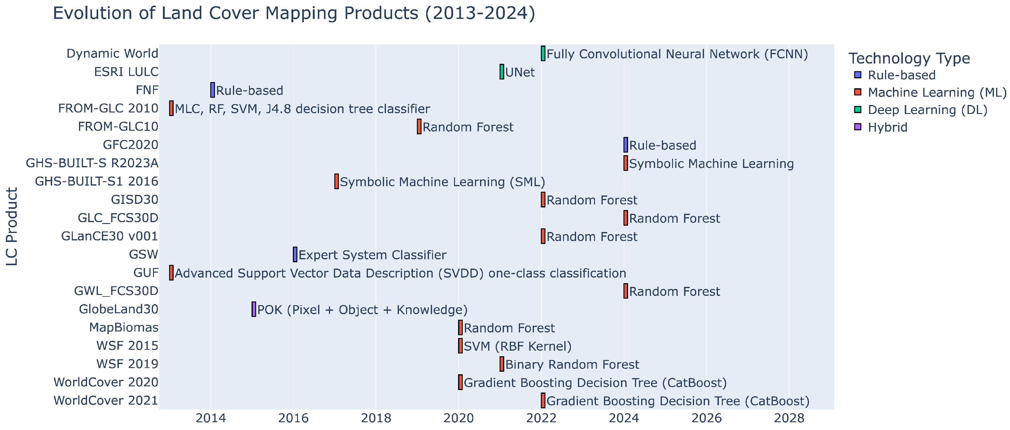
Classification Method	Used In
Random Forest	FROM-GLC30 and FROM-GLC10 [7,31], MapBiomas [38], WSF [40], GISD30 [11], GLanCE v100 [10], GWL_FCS30D [37], GLC_FCS30D [14]
Support Vector Machine	FROM-GLC30 [7], GUF [36], WSF [41]
Gradient Boosting Decision Tree (CatBoost)	WorldCover [18,19]
Symbolic Machine Learning (SML)	GHS-BUILT-S1 2016 [35], GHS-BUILT-S R2023A [34]
Decision Tree	FROM-GLC30 [7]

.

If properly trained, ML methods improve generalization capabilities and can properly model complex scenarios. In traditional machine learning, feature extraction and classification are separated processes. The choice of the features is done in the phase of system design, often relying on specific feature engineering and feature selection strategies. On the contrary, more recent deep learning approaches integrate feature extraction and classification in the learning process, eliminating the need for manual feature extraction design. Furthermore, deep learning can also handle highly complex big data more effectively [49]. The ESRI LULC dataset employs a U-Net deep learning architecture, achieving an overall accuracy of 85% across ten classes [17]. Google’s Dynamic World leverages a fully convolutional neural network (FCNN) to produce near-real-time land cover classifications, with a reported overall agreement of 73.8% between model outputs and expert-labeled data [20].

Despite its advantages, the application of deep learning to global HRLC mapping is still limited. One of the main limitations of these approaches is the requirement to have a very large number of labeled samples in the learning phase. Furthermore, recent advances in attention mechanism-driven deep models, particularly vision transformers (ViT), have sparked a growing interest in their adaptation for LC mapping ([50,51,52]). Given their promising performance in other domains, we look forward to broader adoption of transformer and vision-based AI models for global LC mapping in the future.

3. Legends

A fundamental prerequisite for land cover mapping is the definition of a categorization system for the land cover classes. Different HRLC datasets employ different classification schemes because of varying thematic requirement, regional priorities, and mapping objectives. Some land cover products adopt standardized classification systems directly. For example, FAO Land Cover Classification System (LCCS), a hierarchical framework that define land-cover class by a dynamic combination of classifiers, is utilized by WorldCover. Other products develop entirely customized classification schemes to meet specific mapping requirements, as seen in FROM-GLC30. Meanwhile, some datasets integrate multiple existing standards and/or related products to define their classification schemes. For instance, Dynamic World’s classification scheme was developed through a review of multiple global LULC maps (USGS Anderson classification system [53], ESA Land Use and Coverage Area frame Survey land cover modalities [54], MapBiomas [38], and GlobeLand30 [8]) and designed to align closely with IPCC land use classes [55]. GLC_FCS30D inherits its classification scheme from the CCI_LC products, which, in turn, are based on the FAO LCCS and are compatible with the GLC2000, GlobCover 2005, and 2009 products. Additionally, some datasets integrate regional classification systems to develop more localized classification schemes. For example, MapBiomas employs a hierarchical classification system that merges FAO LCCS with those of the IBGE LCCS, ensuring regional relevance. These differences require a reclassification step to ensure compatibility for comparative analyses. Similarly, GLanCE30 Level 1 classes are similar to the USGS LCMAP classification [56] and align with the IPCC’s top-level land categories for greenhouse gas inventory reporting.

Legend Harmonization

To facilitate inter-comparability or integration, classification system harmonization is required. Crosswalking methods for LC typically assign harmonized LC (HLC) classes to pixels based on votes from source LC (SLC) labels. These methods establish class associations using either binary values (associated or not) (hard association) [20,57,58] or continuous semantic affinity scores (soft association) [59] to measure the thematic correspondence between SLC and HLC classes. While such methods follow predefined rules, they are generally performed manually, requiring domain expertise. This not only makes the process time-consuming but also introduces subjectivity and potential inconsistencies. Furthermore, different HRLC products often adopt different classification systems, resulting in non-corresponding class definitions. For example, the flooded vegetation class in Dynamic World [20] and ESRI LULC [17] includes rice paddies and other heavily irrigated/inundated agriculture, whereas WorldCover incorporates this type of land cover into the cropland class. Similarly, the definition of water varies across these products: WC explicitly specifies a persistency time threshold (more than 9 months) while allowing for certain exceptions, whereas Dynamic World and ESRI LULC lack such constraints [60]. Consequently, linking these categories may introduce uncertainty, leading to inconsistencies not only in cross-comparisons but also in integration. Therefore, standardizing the LC classification system to address differences in LC class definitions and to harmonize class definitions is essential to improve the consistency and comparability of large-scale LC maps.

Furthermore, when comparing different LC products, a relatively simple classification system is often employed to harmonize classes across datasets. This approach typically aggregates fine-grained classes, leading to the loss of specific land types (e.g., wetland subtypes, forest subclasses), which in turn affects the accuracy assessment of these LC products. Additionally, certain LC products demonstrate superior performance in specific categories, and simple class merging may obscure these strengths, introducing distortions in accuracy comparisons. A possible solution to address these challenges is to adopt a multi-level classification scheme [61], allowing for comparisons at varying levels of granularity to better capture differences and maintain classification integrity.

4. Validation

4.1. Sampling Method

In addition to the factors mentioned so far, the reliability of land cover maps also heavily depends on the validation methods employed. In fact, validation methodology inherently involves two important steps: sampling and accuracy assessment. On the other hand, sampling refers to the design protocol for selecting data that serve as a reference (i.e., ground truth) [62] and are used to validate land cover products. Alternatively, accuracy metrics quantify the degree of correctness in classification [62]. In this section, we review recent literature on global land cover validation, examining trends in the use of both sampling and accuracy assessment techniques, as well as potential challenges in their application to global and multi-temporal land cover products. In addition, we present a variety of utilizied sample typologies, which typically depend on the characteristics of data and spatial resolution. These include individual units such as points and pixels, as well as aggregated forms like cells, tiles, and feature-based sampling units, each suited to different validations needs and mapping scales. In

Table 4. Summary of validation sampling approaches and sample sizes from the reviewed studies.

Dataset	Study	Validation Sampling Approach	Number of Validation Samples
DW	Brown et al. [20]	Stratified random sampling by regions and biomes	409 tiles; 1636 annotations
ESRI LULC	Karra et al. [17]	Random stratified sampling of 5 km × 5 km image chips	409 gold standard tiles
FNF	Shimada et al. [30]	Targeted selection from multi-resolution segmentation	4114 points (1456 and 2548 for forest and nonforest, respectively)
FROM-GLC10	Gong et al. [31]	Multi-seasonal sampling; non-systematic training, systematic validation not specified	140,000 validation units
FROM-GLC30	Gong et al. [7]	Non-systematic training; systematic unaligned testing	38,664 test samples
	Yu et al. [32]	Manual sampling from Landsat imagery with MODIS time series	38,664 testing samples
GFC	JRC [33]	Random stratified sampling	49,942 samples
GHS-BUILT-S R2023A	Pesaresi et al. [34]	Stratified sampling	95,210 data blocks of 25 × 25 km size
GHS-BUILT-S1 2016	Corbane et al. [35]	Not applicable	23,134 tiles of 150 × 150 km (using GUF as reference)
GISD30	Zhang et al. [11]	Automated derivation from impervious surface products with refinement rules	23,322 validation samples
GL30	Chen et al. [8]	Two-rank sampling (map sheet and feature sampling)	159,874 pixel samples
GLanCE	Friedl et al. [10]	Simple and stratified random sampling	North America: 1630 reference points
GLC_FCS30/D	Zhang et al. [13]	Automated extraction using CCI_LC and refinement rules; stratified random sampling for validation	44,043 validation samples
	Zhang et al. [14]	Automated training using change detection masks; stratified random sampling with independent datasets for validation	84,526 global validation samples; additional regional datasets (LCMAP, LUCAS)
GSW	Pekel et al. [9]	Stratified random sampling using 1° × 1° grid cells	40,124 control points
GUF	Esch et al. [36]	Randomly distributed sample points; photointerpretation of VHR by GIS experts	2000 for New Delhi; 1500 per each other city mask
GWL_FCS30/D	Zhang et al. [12]	Stratified random sampling for wetland mapping with multi-sourced training	25,709 validation samples
	Zhang et al. [37]	Refinement of a global sample pool with multi-temporal consistency checks; stratified random sampling for validation	Preliminary sample size: 24,000; Final: 22,719 validation points
MapBiomas	Souza et al. [38]	Stratified random sampling; photointerpretation 3 + 1 (senior)	75,000 samples
Tree canopy cover	Hansen et al. [39]	Probability-based stratified sampling; Photointerpretation using Landsat, MODIS and VHR	1500 sampling blocks
WorldCover	Zanaga et al. [18]	Stratified one-stage cluster approach	21,624 PSU (primary sampling unit), 1,935,650 SSUs (secondary sampling units)
	Zanaga et al. [19]	Stratified one-stage cluster approach	21,624 PSU (primary sampling unit), 2,162,366 SSUs (secondary sampling units)
WSF	Marconcini et al. [41]	Stratified random sampling per 1° unit	500 settlement and 500 non-settlement per unit; 900,000 cells total
	Marconcini et al. [40]	Iterative sampling with crowdsourcing validation	180,000 reference cells (WSF-Evolution); 700,000 for WSF2019

, we have compiled the sampling methods and sample sizes used for validation in the reviewed studies focusing on global land cover mapping.

4.1.1. Simple Sampling Method

Simple sampling is a widely used method in which each population unit has an equal chance of being selected. Since there is no further distribution into classes, the final evaluation using the metric is relative to the specific product under assessment. In fact, the biggest disadvantage of this approach is that some dispersed or small population classes may end up being underrepresented. While this method provided a validation baseline, certain limitations were evident, such as the potential for uneven representation of certain land cover classes and the reliance on single-date imagery.

Scholars, such as Foody [63], emphasize that simple random sampling can be considered suitable without compromising the reliability of the final product, but only when all land cover classes are sufficiently represented in the population sample. Moreover, it is suggested to take into account potential constraints related to the study area during the design process and to avoid random sampling when working with large areas [63]. Nevertheless, it is a highly versatile approach that can be easily adopted in combination with other methods, such as stratified or cluster sampling [64].

4.1.2. Stratified Sampling Method

Beyond simple random sampling, stratified sampling is another widely used technique Table 4. The goal of this approach is to group the samples into distinct strata, ensuring that each sample belongs to a single stratum [64]. Two main types of strata discrimination can be distinguished: one based on map class and the other on spatial location. The former allows for the increased representation of rare land cover types, while the latter enhances representation for specific, usually small areas or helps introducing a spatially balanced sample [64]. In either case, the implementation of this approach improves the statistical reliability of accuracy assessments by generating precise accuracy estimates for each class.

Among the various implementations of this method, a few studies stand out for integrating additional criteria. For instance, in the case of Dynamic World, Brown et al. [20] divided the world into three regions (Western Hemisphere, Eastern Hemisphere-1, and Eastern Hemisphere-2), further subdividing each region into 14 biomes and using an auxiliary land cover dataset for stratification.

Chen et al. [8] detailed a two-rank sampling strategy for GlobeLand30, involving both map sheet sampling and feature sampling. In the first rank, map sheets (6° × 5° grids) were selected from a global inventory of 847 sheets covering all continents. In the second rank, feature samples of each land cover type were selected using spatial stratification sampling within the chosen map sheets.

4.1.3. Systematic Sampling Method

Systematic sampling is another basic method for sample selection, where representative units are defined at regular intervals [64]. It is usually applied when the aim is to achieve spatial balance, ensuring that the area of interest has a well-distributed numerical coverage. Some advantages of this method include its ease of implementation and, in contrast to simple random sampling, its ability to improve population variability by reducing potential sample clustering. On the other hand, its implementation may lead to periodicity bias if the selected interval coincides with a pattern in the population. A more robust alternative to systematic sampling is the use of the stratified method [65].

In fact, from the reviewed studies focused on global land cover mapping (Table 4), it is evident that systematic sampling is not a favoured methodology. The only notable implementation is found in Gong et al. [7], where the authors applied systematic unaligned sampling by first dividing the globe into approximately 7000 equal-area hexagons. They then assigned different sample counts: 10 per hexagon for Europe and China, and 5 for the rest of the world. The final sample collection resulted in more than 35,000 valid samples.

4.1.4. Clustered Sampling Method

Clustered sampling is a methodology that involves dividing the population into small groups (clusters). Two distinct approaches are often adopted: one-stage cluster sampling, where sampling is conducted directly on the primary clustered units, and two-stage cluster sampling, where samples are selected within the primary clusters [62,64]. One of the key advantages of its implementation is cost-effectiveness, as once an interpretation is made for a pixel within a cluster, the effort required for an additional one in the same group is significantly lower [62].

An example of such sampling can be seen in the methodology applied by Marconcini et al. [41] for validating the World Settlement Footprint. In this approach, an initial clustering of tiles (each 1° × 1° in size) was conducted, followed by the selection of 50 tiles which can be interpreted as clusters. Finally, individuals from both classes (settlement and non-settlement) were sampled within the selected tiles.

Moreover, clustering can be carried out not only spatially but also using additional criteria. To augment their training samples, Friedl et al. [10] applied unsupervised clustering based on spectral-temporal features using Landsat time-series imagery.

4.1.5. Sample Typologies

The types of validation samples reported in the previous studies (see Table 4) vary widely depending on the nature of the dataset and the spatial resolution of the derived products. Based on the reviewed literature, several main typologies can be highlighted. At the most basic level, points also referred as reference control points are used to represent precise ground locations, as illustrated in GLanCE [10]. When going to a slightly broader sample type, the individual sample is still noted, with the usage of pixels being the smallest units (e.g., used in GL30 [8] in raster images allowing detailed per-pixel accuracy assessment. Moving beyond individual units, many studies employ aggregated sample types such as cells (e.g., WSF [41]), data blocks (GHS-BUILT-S R2023A [34]), and sampling units (WorldCover [18,19]). The former two usually appear to be with more regular size, while the sampling units can be based on spatial units, they can be derived be on some feature-based units (e.g., water or forest bodies) or even on hierarchic units (as in WorldCover). Another commonly used sampling typology is tiles which a larger patches typically extracted from satellite imagery (as in DW [20] or aerial photographs. Each sample type server has different validation needs. Individual units such as points and pixels offer high spatial precision, while aggregated units such as tiles or data blocks capture broader spatial patterns; however, they may smooth out local variability. The selection of a sampling unit should consider both the spatial resolution and the intended scale of the output products to ensure alignment with the map’s level of detail.

4.2. Sample Size Selection

The selection of an appropriate sample size is an integral and crucial step in the validation design of many spatial analyses, including global and regional land cover mapping. Among the empirical general rules we mention the proposition by Hay et al. [66], which recommends including at least 50 samples per category for which accuracy is tested. However, later it was clarified that this rule [67] should be followed only when the area of interest is under 500,000 ha and less than 12 thematic classes are present [68].

In the literature, two statistically based criteria are favored during the design process. A widely used approach is the formula proposed by Cochran [69], which ensures that the total estimated sample size is reliable within a certain confidence level and error margin. A more refined method, particularly focused on the sample size per stratum [69,70], uses the overall sample size while also considering the permissible error level and the proportion of the stratum covering the study area. This leads to weighted sample selection and better allocation in underrepresented classes, effectively addressing the issue of accuracy imbalance. Olofsson et al. [70] further proposed a simplified iterative sample size selection method by initially assigning a minimum of 50 samples for a rare stratum and monitoring the anticipated standard errors of accuracy. The process is iteratively adjusted until the desired precision levels for accuracy are achieved. This approach ensures efficient allocation while minimizing variance without introducing bias into the estimators.

Among the reviewed literature on global land cover mapping, all scholars have reported the sample size used for validation (Table 4). However, it is notable that not all studies have explicitly discussed the motivation behind the final sample size selection. Naturally, many applications are based on the requirement that the selected population should satisfy a certain error margin or class-specific accuracy (e.g., [8,12,30,59]).

Some studies have conducted experiments by adjusting their sample sizes to quantitatively analyze the effect on final accuracy. Gong et al. [7] modified their test sample size in a cluster and found that varying the number of samples did not lead to drastic changes in the final accuracies.

On the other hand, it can be noted the use a sample size that directly results from the application of additional design criteria. An example is the creation of the population used in validating the Dynamic World product [20], where the actual product is not based on a single static image classification but rather on a temporal basis using Sentinel-2 scenes. Here the validation set is a product of a more complex training/testing dataset definition, comprising spatial and thematic stratification, followed by expert and non-expert annotations. Similarly, Marconcini et al. [41] implemented a percentile-based criterion for tile selection based on the ratio between the number of settlements and their overall area. Similarly, the works by Zhang [11,37] applied automated procedures and rule-based criteria to define validation samples, often incorporating sampling informed by auxiliary datasets. Such approaches highlight the trend of integrating more structured and data-driven design choices to support large-scale validation efforts.

4.3. Sample Interpretation

Another important step in validation design, directly related to sample generation, is sample interpretation. In the land cover mapping domain, this refers to assigning a reference land cover class to each unit. From the reviewed works on global land cover mapping, several approaches can be highlighted, ranging from more traditional and well-established methods (e.g., photo interpretation) to more innovative automated ones (e.g., property-based clustering), each with its own strengths and weaknesses.

4.3.1. Manual Interpretation

Manual interpretation typically relies on human annotators classifying samples according to land cover classes. In many cases, these interpretations are desktop-based, using high-resolution remotely sensed imagery, which generally allows for faster class identification. Some works [8] highlight the added benefits of class-specific, nature- and culture-based local knowledge. Nevertheless, the majority of studies rely on high-resolution photo interpretation, which can be further categorized into expert [7,10,11,14,20,36] and non-expert approaches [14,20]. A comparable methodology is applied in Souza et al. [38], where the initial labeling is carried out by three interpreters, and any disagreements are resolved by a senior expert who determines the final land cover classification.

The use of expert knowledge, particularly the involvement of multiple photointerpreters, is critical for improving the quality of training and test samples. Engaging trained professionals with expertise in land cover classification, remote sensing, and specific software tools typically leads to more consistent and accurate datasets. Additionally, the participation of multiple annotators results in more refined samples with higher confidence in their class attribution. For example, Gong et al. [7] involved more than 20 trained annotators at different stages of the interpretation process, based on their evaluated performance. Furthermore, their design process included a confidence classification to filter out samples where annotators were highly uncertain about the assigned class.

On the other hand, including non-experts in the interpretation process is generally beneficial for large-scale projects, where the number of samples to be processed is significantly high. This approach often prioritises “quantity over quality” and necessitates further quality assessment of the output samples. A similar methodology was applied in [20], where three experts and one non-expert were involved to benefit from cross-expert quality evaluation, further balancing accuracy with labeling efficiency. Zhang et al. [14] involved multi-level experts to independently interpret validation samples; however, the results from junior annotators required further cross-checking.

4.3.2. Automated Interpretation

Methodologies for automatic sample interpretation (or creation) have emerged in recent years, with some examples leveraging data augmentation through unsupervised spectral clustering, which still requires photo interpretation [10]. These approaches have the potential to reduce the time required for sample generation. Other researchers have integrated auxiliary land cover products to generate training samples, using multiple land cover datasets and their points of agreement to create highly accurate training samples [57]. Similar auxiliary data have also been employed in global studies [11,12]. Zhang et al. [11] implemented a spectral-generalization strategy for training set creation, although manual interpretation was still required for accuracy assessment. However, while such automated approaches are widely favored for training set compilation, validation sets continue to rely primarily on manual interpretation.

4.3.3. Imagery Data Used for Interpretation

As seen in the previous section, class annotation of reference samples using photo interpretation is a crucial step in all global studies. This process is directly linked to the dataset used and the requirements it must satisfy. One of the main data sources, optical imagery, presents certain limitations, such as cloud cover, resolution constraints, and spectral differences. To overcome these limitations, scholars often rely on multi-source and multi-resolution imagery. Upon review, it is notable that a few high- and medium-resolution datasets are frequently used for land cover class interpretation.

Table 5. Summary of data sources used for photo-interpretation.

Data Source	Resolution	Advantages	Used In
Landsat	30 m (Multispectral), 15 m (Panchromatic)	Long-term data record, time-series analysis, surface reflectance, identification of land cover dynamics	FROM-GLC30 [32], GHS-BUILT-S1 2016 [35], GL30 [8], GLC_FCS30/D [14,59], GLanCE [10], MapBiomas [38], Tree canopy cover [39]
Google Earth VHR Imagery	0.15 m to 1.5 m (Varies depending on source)	Very high spatial resolution, validation of other satellite data, reference data source	FNF [30], FROM-GLC30 [32], GLC_FCS30/D [14,59], GLanCE [10], GUF [36], MapBiomas [38], Tree canopy cover [39], WSF [41]
Sentinel-2	10 m, 20 m, 60 m (Varies by band)	High spatial, spectral, and temporal resolution, surface reflectance, land cover classification	ESRI LULC [17], GHS-BUILT-S1 2016 [35], GLC_FCS30/D [14]
MODIS	250 m to 1 km (Varies by product)	Time series vegetation indices (e.g., NDVI, EVI), extraction of seasonal vegetation information	FROM-GLC30 [7], FROM-GLC30 [32], GL30 [8], GLC_FCS30/D [59], GLanCE [10], MapBiomas [38], Tree canopy cover [39]

summarizes our findings regarding the most commonly used optical datasets for image interpretation. It is evident that the most favored dataset source is the Landsat mission, primarily due to its provision of long-term medium-resolution data suitable for historical dynamic analyses. This is followed by Google Earth, which offers open access to very high-resolution images and, in many locations, provides relatively long time-series information. Notably, Sentinel-2 was used less frequently for sample interpretation compared to Landsat, despite its higher spatial and temporal resolution. This finding may be explained by the fact that the first Sentinel-2 satellite was launched in 2015 and the second in 2017, rendering the mission relatively “recent” with a more limited data archive compared to some of the works reviewed here. The last frequently implemented source is the MODIS mission, which, despite the moderate resolution, is highly suitable for extracting seasonal vegetation information and is favored for its exceptionally high temporal resolution (1–2 days).

It should be noted that not all of the reviewed papers were included in Table 5, even if they utilized optical imagery for reference. This is mainly because, in some cases, the specific data source was not explicitly mentioned. Conversely, some studies did not rely on optical imagery at all. Instead, certain works used domain-specific thematic auxiliary datasets, such as reference data with high “assumed” level of correctness [34], or other land cover products, such as ESA CCI LC [14].

4.3.4. Crowdsourced Data

Crowdsourced data has emerged as a valuable tool in land cover validation, enabling researchers to collect large-scale samples remotely from various geographic regions by leveraging contributions from both experts and non-experts. Furthermore, crowdsourced data supplements traditional validation methods with significantly greater availability of human-labeled data, utilizing tools such as mobile apps (which provide high-resolution in-situ data) and online collaborative platforms (which allow for remote assessments).

It is evident that this approach could further support efforts to validate global land cover maps, as it has been implemented in a few of the reviewed works. For example, Friedl et al. [10] incorporated crowdsourced data, while Gong et al. [7] suggested using the GeoWiki global database of crowdsourced land cover sites [71]. This resource contains a vast amount of annotated cells (>150 million), yet further processing is required for case-specific applications. Similarly, after refinement, Zhang et al. [59] incorporated a class-specific dataset (global cropland reference data) obtained via crowdsourcing. Marconcini et al. [41] also harnessed the collective power of crowdsourcing through an unprecedented photo-interpretation campaign, annotating 900,000 samples using very high-resolution imagery. However, the reliability of crowdsourced data strongly depends on the definition of the land cover type, as broader, more general classes tend to be easier for non-expert contributors to interpret consistently. In contrast, a detailed legend with many specific categories may lead to confusion and misclassification, especially in the absence of expert guidance. This is particularly relevant when considering the experience level of the photo-interpreter, as trained professionals are typically better equipped to handle nuanced distinctions in land cover types than the general public.

4.4. Accuracy Metrics

The assessment of accuracy in land cover maps relies not only on the design choices made during the sampling process but also on the metrics used to quantify how well a classification model represents reality. The process of global land cover mapping has evolved significantly, and it is evident that scholars are shifting from simple agreement measures to more refined statistical indices that account for spatial and class-specific variations.

To better understand the frequency of usage of these metrics, we conducted a quantitative assessment based on the reviewed studies. Initially, we are reporting the metrics used per global product (see

Table 6. Summary of the used validation metrics from the reviewed studies. OA—Overall accuracy; UA—User accuracy; PA—Producer accuracy; Kappa; CE—Commission error; OE—Omission error; F1; AA—Average accuracy; Var (K)—Variance of K. The red-to-green colour scheme visually highlights the total count of metrics used per paper, with red indicating the fewest and green the most.

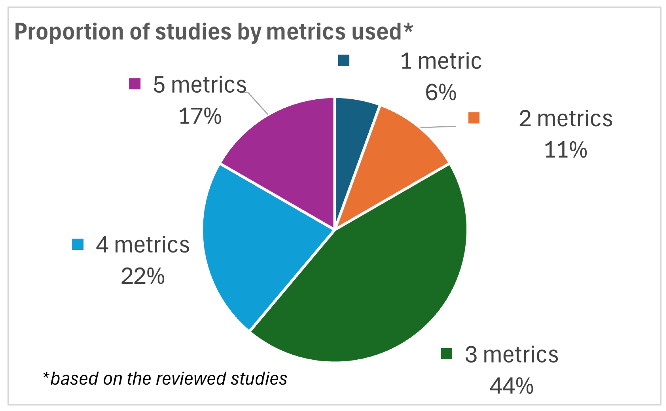
Dataset	OA	UA	PA	Kappa	CE	OE	F1	AA	Var(K)	Total per Product
DW [20]	X	X	X							3
ESRI LULC [17]	X	X	X							3
FNF [30]	X									1
FROM-GLC10 [31]	X	X	X							3
FROM-GLC30 [7,32]	X	X	X	X					X	5
GFC [33]	X	X	X		X	X				5
GHS-BUILT-S R2023A [34]	not applicable									3
GHS-BUILT-S1 2016 [35]				X	X	X				3
GISD30 [11]	X	X	X	X						4
GL30 [8]	X	X	X	X						4
GLanCE [10]	X	X	X							3
GLC_FCS30/D [13,14]	X	X	X	X			X			5
GSW [9]					X	X				2
GUF [36]	X	X	X	X						4
GWL_FCS30/D [12,37]	X	X	X	X						4
MapBiomas [38]	X	X	X							3
Tree canopy cover [39]	X	X	X							3
WorldCover [18,19]	X	X	X							3
WSF [41]		X	X	X				X		4
Total per metric	15	15	15	8	3	3	1	1	1

). In addition, the last column and row are highlighting the trends and preferences in selecting validation metrics. Notably, the majority of works rely on at least three or more validation metrics (Figure 3). In contrast, only one of the reviewed studies [30] validated its results using a single indicator. To explain the interest in multiple validation metrics in the reviewed studies, we further explored the types of metrics implemented. The last row of Table 6 represents the number of times each metric was used across different studies. Overall, the trends suggest a shift away from relying solely on aggregated indices, such as overall accuracy or kappa.

The evaluation approach used for GHS-BUILT-S R2023A [34] differs from the other studies because it focuses on a continuous dataset, whereas the others evaluate categorical outputs. Consequently, the authors selected validation metrics suited to continuous data, namely, R-accuracy, Mean Absolute Error (MAE), and the Jaccard similarity index (IoU). R-accuracy and MAE assess the level of agreement and the magnitude of errors between predicted and reference continuous values, while IoU was applied in a ROC analysis to determine the optimal threshold for converting continuous predictions into binary classifications.

As global land cover classification processes become increasingly complex—both spatially and thematically—it has become evident that no single metric can fully capture classification performance. As a result, studies are implementing multiple complementary metrics to provide a more well-rounded evaluation while also offering better class-specific insights. In fact, the overall trends indicate a clear focus on the latter, with user’s and producer’s accuracies emerging as the most favored, as they provide direct insights into both omission and commission errors. Unfortunately, upon reviewing the studies it was not possible to determine a clear temporal pattern in terms of validation.

Naturally, scholars also tend to implement generalized metrics, such as overall accuracy or kappa, which, while useful, can sometimes overlook important classification details. A key example is the widespread use of overall accuracy, which, despite being a common measure, has limitations in handling class imbalances. Therefore, it is considered good practice to supplement it with class-specific evaluations. Similarly, Kappa is generally regarded as a more robust measure complementary to class-specific metrics, as it accounts for the possibility of agreement occurring by chance and considers class imbalance. However, its limited usage is often attributed to its less intuitive interpretation and sensitivity to class sample size.

To address this issue Yu et al. [32] implement the variance of kappa (Kvar) to adjust for the influence of dominant classes, potentially making Kappa more interpretable when class prevalence varies significantly. Despite being well-suited for unbalanced classes and better founded than Kappa for accuracy assessment, the F1-score remains rarely used, appearing in only one of the reviewed studies [14]. Such limited implementation suggests that it has not yet become a standard metric in global land cover classification.

The practice of implementing multiple validation measures in combination is likely to persist, as the field of land cover classification (e.g., models and datasets) continues to evolve, reflecting broader trends in remote sensing and machine learning. Future studies are expected to continue evaluating classification performance at the class level rather than relying solely on singular global metrics.

5. Data Distribution and Cloud Platforms

5.1. Data Distribution

The accessibility and distribution of land cover mapping products play a critical role in their utilization across scientific research, environmental monitoring, and policy decision-making. The access points of all studied HRLCs in this paper can be found in

Table A1. Access points of HRLCs involved in this study.

Dataset Name	Access Point
GLC_FCS30D	https://zenodo.org/records/8239305 (accessed on 26 February 2025)
GWL_FCS30D	https://zenodo.org/records/10068479 (accessed on 26 February 2025)
GISD30	https://zenodo.org/records/5220816 (accessed on 26 February 2025)
Dynamic World	GOOGLE_DYNAMICWORLD_V1 (accessed on 26 February 2025)
ESRI LULC	https://livingatlas.arcgis.com/landcover/ (accessed on 26 February 2025)
WorldCover	https://esa-worldcover.org/en/data-access (accessed on 26 February 2025)
GLanCE v001	https://lpdaac.usgs.gov/products/glance30v001 (accessed on 26 February 2025)
GlobeLand30	https://cloudcenter.tianditu.gov.cn/landCover (accessed on 26 February 2025)
FROM-GLC30	https://data-starcloud.pcl.ac.cn/ (accessed on 26 February 2025)
FROM-GLC10	https://data-starcloud.pcl.ac.cn/ (accessed on 26 February 2025)
World Settlement Footprint (WSF)	WSF2019 (accessed on 26 February 2025)
MapBiomas	https://brasil.mapbiomas.org/en/colecoes-mapbiomas/ (accessed on 26 February 2025)
GSW	https://global-surface-water.appspot.com/download (accessed on 26 February 2025)
GUF	https://www.dlr.de/en/eoc/research-transfer/projects-missions/global-urban-footprint/guf-data-and-access (accessed on 26 February 2025)
GHS-BUILT-S R2023A	GHS-BUILT-S R2023A (accessed on 26 February 2025)
GHS-BUILT-S1 2016	GHS-BUILT-S1 2016 download link (accessed on 26 February 2025)
GFC	https://forobs.jrc.ec.europa.eu/GFC (accessed on 26 February 2025)
FNF	FNF download link (accessed on 26 February 2025)
Tree canopy cover	hansen_global_forest_change (accessed on 26 February 2025)

.

Cloud-based platforms are now widely used for sharing and analyzing land cover data. They allow users access and process datasets without storing them locally. Google Earth Engine (GEE) is one of the most popular platforms. It hosts many datasets like GFC, FNF, and Dynamic World [20]. Amazon Web Services (AWS) Open Data also provides access to large-scale datasets, including GLanCE30 and GSW. These platforms help users to easily analyze data in the cloud.

Other than cloud platforms, some open data repositories give direct access to land cover datasets. Zenodo, for example, hosts land cover products like GLC_FCS30D and GISD30. It also provides DOI references so that researchers can cite and reuse the data. The China National Platform for Common Geospatial Information Services offers GlobeLand30 data to authorized users, making sure the distribution is controlled.

Many land cover datasets can be accessed through multiple ways. For instance, GSW data is available not only via GEE but also through the JRC portal, where users can manually select and download specific tiles or retrieve data via FTP services. ESA WorldCover, on the other hand, provides even more access options, including the WorldCover viewer, Terrascope, AWS S3 bucket, Zenodo, and GEE, accommodating various user preferences.

Land cover products are distributed in multiple formats to support different requirements. Raster-based formats like GeoTIFF are often used for direct spatial analysis. Some platforms also provide Web Map Services (WMS), which let users use the data in GIS platforms. Data availability is not the same for all products. Most datasets, such as ESA WorldCover, are freely available. Others, like GUF, need special permission to access.

The diversification of data distribution mechanisms allows users to select platforms and retrieval methods based on their needs, significantly enhancing data availability and usability across disciplines.

5.2. Trends in Platform Usage

GHRLC classification is a complex and resource-intensive task, requiring extensive data preprocessing, high performance computing, and high-quality training data to ensure both local reliability and global consistency [72].

Some LC products are generated using custom-developed platforms and computational environments. For instance, GUF dataset was produced using the Urban Footprint Processor, implemented at the German Remote Sensing Data Center (DFD) of the German Aerospace Center (DLR), generating a very high-resolution global human settlements layers at a spatial resolution of approximately 12 m [36]. Similarly, GHS-BUILT-S1 2016 was created using JRC Earth Observation Data and Processing Platform, designed for Earth observation (EO) data storage and processing [35].

Given the immense computational demands of large-scale LC mapping, many projects rely on supercomputers. For example, in WSF2015, the computation of Landsat-8 temporal statistics, training point extraction, and classification tasks was performed at the IT4Innovations Czech supercomputing center [41]. Likewise, all image classification tasks for FROM-GLC2010 were executed on the Tsinghua University supercomputer [7].

However, this on-premise computing relies on local computers and is limited by computing power, storage space, and data download costs. Therefore, more and more LC mapping tasks are performed on cloud-based computing platforms, which enable efficient processing without the need for local high-performance computing infrastructure. For example, ESRI LULC utilized the Microsoft Planetary Computer and Microsoft Azure Batch to process over 20,000 Sentinel-2 tiles, which covers the entire Earth’s land surface [17].

Among cloud-based platforms, Google Earth Engine (GEE) has become one of the most widely used due to its multi-petabyte data catalog, high-performance parallel computing capabilities, and extensive image-processing libraries that perform pixel-wise algebraic operations [73]. This, coupled with its ability to provide efficient and free access to a large number of remote sensing datasets, has led to its increasing use in HRLC classification. Take Dynamic World as an example: it uses cloud computing on GEE and Google Cloud AI Platform to generate near real-time predictions of LULC class probabilities for new and historical Sentinel-2 images [20]. The expert system used by GSW, if executed on a single CPU, would have required approximately 1212 years to complete. By using 10,000 parallel computers on the GEE platform, the processing time was dramatically reduced to about 45 days [9].

Although cloud-based platforms have significantly improved efficiency, they still have several notable limitations. For example, GEE is constrained by compute limits, lack of processing algorithms and data, and limited flexibility of different models [74].

6. Discussing Current Trends and Future Directions

6.1. Multi-Source Data Fusion

Numerous studies [9,10,11,12,14,33] have highlighted that the accuracy of LC mapping is significantly influenced by both the availability and quality of Landsat data. Moreover, due to the limited temporal coverage of Sentinel-2 imagery, Dynamic World can only provide HRLC data starting from 2015. A promising solution to these limitations is data fusion, which involves integrating multiple data sources, including multi-sensor or multi-resolution datasets, to enhance the accuracy and reliability of LC classification. Jin and Mountrakis (2022) [75] show that combining spaceborne optical data (Landsat-5/TM), SAR data (ALOS-1/PALSAR), and airborne full-waveform LiDAR (LVIS) significantly improves the discrimination of different land cover types. Beyond remote sensing data, auxiliary datasets have also proven valuable. For instance, Marconcini et al. (2021) [40] leveraged OpenStreetMap (OSM) data along with a novel dataset from Facebook that predicts missing roads in OSM to effectively mask out roads, thereby refining classification accuracy.

Future research should aim to develop standardized frameworks for harmonizing data from different sensors across space and time. It should also explore adaptive fusion strategies capable of dynamically responding to regional data availability and land cover complexity. Moreover, the integration of new data sources, such as high-revisit commercial satellites and crowdsourced geospatial information, has great potential to further enhance classification robustness, particularly in regions with sparse historical observations.

6.2. High Resolution and Real-Time Mapping

Despite significant advancements, real-time HRLC mapping remains a critical gap. Most of the HRLC products discussed in this study are annual maps, capturing LC conditions from past years, which limits their applicability for dynamic monitoring. A notable exception is Google’s DW, the first GHRLC product capable of near-real-time updates. However, its performance varies across time and space, influenced by Sentinel-2 cloud cover quality and variability in land cover conditions. Meanwhile, the increasing availability of higher-resolution satellite imagery has paved the way for LC products with enhanced spatial accuracy. For instance, Basheer et al. (2024) [76] achieved an overall classification accuracy of up to 94% for six land cover classes by using PlanetScope imagery (3-m spatial resolution) and four supervised classifiers (SVM, ML, RF, and KNN). Thus, further improvements in both the spatial and temporal resolution of LC products remain a key priority for future research and development.

Future work should explore adaptive processing pipelines for near real-time updates using cloud-free imagery from multiple sensors, as well as investigate incremental learning frameworks that enable efficient integration of new observations without requiring complete model retraining.

6.3. Computational Challenges

The increasing availability of high-resolution satellite imagery brings not only opportunities but also significant challenges for HRLC mapping. While these data enhance the potential for more precise land cover classification, they also place substantial demands on computational resources. Advanced algorithms, particularly deep learning models, on the other hand, have significantly improved classification accuracy but require robust computing power and efficient data processing pipelines. Although cloud-based platforms such as GEE have been widely adopted for HRLC mapping, they still face limitations, including constrained computational resources, a limited range of available algorithms, and incomplete data sources. To solve these problems, cloud platforms should keep improving by offering more types of algorithms, larger and more complete datasets, and better support for advanced AI tools like PyTorch and TensorFlow. This will help make high-resolution land cover mapping faster and more accurate.

6.4. Standardized Datasets and Validation Protocols/Frameworks

Our review highlighted the diversity of sampling methods used in global land cover validation, with stratified random sampling emerging as one of the most widely preferred approaches for creating the reliable samples used for accuracy computations. Mainly, this is due to the fact the method efficiently addresses class imbalances and enhances statistical reliability. Moreover, systematic and clustered sampling methods offer certain advantages, such as spatial balance and cost-effectiveness, thus, their practical application to large-scale studies is notable. With regard to sample annotations, manual photo-interpretation (whether it is expert or non-expert based) continues to be the dominant method, as it can offer s highly-accurate reference dataset (especially when cross-referenced), naturally, with the cost of a high manual and time-consuming workload. However, automated techniques, such as spectral clustering and the integration of auxiliary datasets, are emerging, offering a more scalable approach for augmented spatially distributed population samples. Similarly, accuracy assessment has evolved beyond simple overall accuracy metrics, with an increasing focus on class-specific measures, such as user’s and producer’s accuracies, which provide deeper insights into classification errors and model performance.

Despite these approaches emerging as a standard in land cover validation, the lack of standardized, high-quality reference datasets remains a significant challenge. Already, Li et al. [77] has demonstrated that an all-seasons sample dataset brings a significant improvement of the classification outputs across the different temporal epochs. Similarly, Fritz et al. [71] highlighted the potential of crowdsourced land cover data as a scalable and cost-effective means of collecting validation samples. Establishing globally consistent, multi-temporal reference datasets will not only improve model validation methodologies but will also ensure greater reliability across different classification products and facilitate better intercomparison between land cover datasets.

Another key obstacle to comparability between different land cover classification products lies in the differences in land cover nomenclature used by different products. As discussed in Section 2, these nomenclatures vary widely-ranging from standardized systems like the FAO LCCS to completely custom or hybrid schemes-posing considerable challenges for direct comparison. To address this issue, legend harmonization is required. However, as outlined in Section 2.1, it often involves a degree of subjectivity and may lead to inconsistencies. Consequently, future work should focus on developing community-agreed nomenclature standards or machine-readable ontological frameworks that enable objective and scalable intercomparison between LC products.

7. Conclusions

This review provides a comprehensive analysis of the data sources, methodologies, and validation techniques utilized in 19 binary or multi-class GHRLC products. It examines the usage of data sources and the preprocessing methods, from reliance on single-input datasets to the integration of satellite optical/SAR and other geospatial data. Optical imagery remains the primary input, while radar data are sometimes used to obtain valuable information about surface structure and moisture. Preprocessing steps such as radiometric/geometric correction, cloud masking, image fusion, and resampling significantly affect the reliability of classification. Additionally, it summarizes the progression of GHRLC production techniques, from early rule-based approaches to the widespread use of ML algorithms, particularly RF and SVM, which currently dominate the implementations. More recently, deep learning models such as U-Net and FCNN have been explored to capture more complex spatial patterns. More and more LC products leverage the computational power of cloud-based platforms, and GEE is one of the most widely adopted platforms.

A key focus of this review is the ongoing challenge of land cover legend harmonization, a crucial issue for ensuring consistency and comparability across datasets. The absence of a standardized legend system limits effective comparison among different LC products, making it difficult to integrate or evaluate them in a unified framework. Another fundamental aspect discussed is validation, which remains essential for assessing the accuracy and reliability of GHRLC products. The paper explores various validation methods, including statistical approaches and visual inspections, and highlights recent advancements in validation protocols, underscoring their role in maintaining data integrity and addressing emerging requirements, such as the development of standardized validation datasets. In particular, our analysis highlights that also in this case there is no standardized sampling approach. However, stratified approaches tend to emerge as most preferable as they enhance class representation and reduce bias, while clustered or systematic techniques may introduce spatial dependencies or sampling inefficiencies.

Despite significant progress, challenges persist in areas such as data completeness, real-time processing, and reliable validation. Potential solutions include data fusion, enhancements of cloud-based platforms, and the establishment of standardized validation datasets and protocols.Looking ahead, future research on GHRLC mapping should prioritize the development of standardized frameworks to enable data harmonization across sensors, spatial scales, and temporal resolutions. Adaptive data fusion and processing strategies are critical to address regional heterogeneity and support near-real-time updates. Incremental learning frameworks that can incorporate new observations without full model retraining are also worthy of further exploration. At the same time, cloud platforms are expected to continue to evolve, providing a wider selection of algorithms, more comprehensive datasets, and strong support for advanced AI frameworks. It is also important to establish standardized validation datasets and protocols, which are critical to ensuring consistent assessments and promoting comparability across products. Together, these directions will support the creation of more timely, accurate, and reliable land cover products for a variety of environmental and policy applications.

References

- Sheykhmousa, M.; Kerle, N.; Kuffer, M.; Ghaffarian, S. Post-disaster recovery assessment with machine learning-derived land cover and land use information. Remote Sens. 2019, 11, 1174. [Google Scholar] [CrossRef]
- Ghaffarian, S.; Rezaie Farhadabad, A.; Kerle, N. Post-disaster recovery monitoring with google earth engine. Appl. Sci. 2020, 10, 4574. [Google Scholar] [CrossRef]
- Gaur, S.; Singh, R. A comprehensive review on land use/land cover (LULC) change modeling for urban development: Current status and future prospects. Sustainability 2023, 15, 903. [Google Scholar] [CrossRef]
- Carter, S.; Herold, M. Specifications of Land Cover Datasets for SDG Indicator Monitoring. 2019. Available online: https://ggim.un.org/documents/Paper_Land_cover_datasets_for_SDGs.pdf (accessed on 25 February 2025).
- Roy, P.S.; Ramachandran, R.M.; Paul, O.; Thakur, P.K.; Ravan, S.; Behera, M.D.; Sarangi, C.; Kanawade, V.P. Anthropogenic land use and land cover changes—A review on its environmental consequences and climate change. J. Indian Soc. Remote Sens. 2022, 50, 1615–1640. [Google Scholar] [CrossRef]
- Szantoi, Z.; Geller, G.N.; Tsendbazar, N.E.; See, L.; Griffiths, P.; Fritz, S.; Gong, P.; Herold, M.; Mora, B.; Obregón, A. Addressing the need for improved land cover map products for policy support. Environ. Sci. Policy 2020, 112, 28–35. [Google Scholar] [CrossRef]
- Gong, P.; Wang, J.; Yu, L.; Zhao, Y.; Zhao, Y.; Liang, L.; Niu, Z.; Huang, X.; Fu, H.; Liu, S.; et al. Finer resolution observation and monitoring of global land cover: First mapping results with Landsat TM and ETM+ data. Int. J. Remote Sens. 2013, 34, 2607–2654. [Google Scholar] [CrossRef]
- Chen, J.; Chen, J.; Liao, A.; Cao, X.; Chen, L.; Chen, X.; He, C.; Han, G.; Peng, S.; Lu, M.; et al. Global land cover mapping at 30 m resolution: A POK-based operational approach. ISPRS J. Photogramm. Remote Sens. 2015, 103, 7–27. [Google Scholar] [CrossRef]
- Pekel, J.F.; Cottam, A.; Gorelick, N.; Belward, A.S. High-resolution mapping of global surface water and its long-term changes. Nature 2016, 540, 418–422. [Google Scholar] [CrossRef]
- Friedl, M.A.; Woodcock, C.E.; Olofsson, P.; Zhu, Z.; Loveland, T.; Stanimirova, R.; Arevalo, P.; Bullock, E.; Hu, K.T.; Zhang, Y.; et al. Medium Spatial Resolution Mapping of Global Land Cover and Land Cover Change Across Multiple Decades from Landsat. Front. Remote Sens. 2022, 3, 894571. [Google Scholar] [CrossRef]
- Zhang, X.; Liu, L.; Zhao, T.; Gao, Y.; Chen, X.; Mi, J. GISD30: Global 30 m impervious-surface dynamic dataset from 1985 to 2020 using time-series Landsat imagery on the Google Earth Engine platform. Earth Syst. Sci. Data 2022, 14, 1831–1856. [Google Scholar] [CrossRef]
- Zhang, X.; Liu, L.; Zhao, T.; Chen, X.; Lin, S.; Wang, J.; Mi, J.; Liu, W. GWL_FCS30: A global 30 m wetland map with a fine classification system using multi-sourced and time-series remote sensing imagery in 2020. Earth Syst. Sci. Data 2023, 15, 265–293. [Google Scholar] [CrossRef]
- Zhang, X.; Liu, L.; Chen, X.; Gao, Y.; Xie, S.; Mi, J. GLC_FCS30: Global land-cover product with fine classification system at 30 m using time-series Landsat imagery. Earth Syst. Sci. Data 2021, 13, 2753–2776. [Google Scholar] [CrossRef]
- Zhang, X.; Zhao, T.; Xu, H.; Liu, W.; Wang, J.; Chen, X.; Liu, L. GLC_FCS30D: The first global 30 m land-cover dynamics monitoring product with a fine classification system for the period from 1985 to 2022 generated using dense-time-series Landsat imagery and the continuous change-detection method. Earth Syst. Sci. Data 2024, 16, 1353–1381. [Google Scholar] [CrossRef]
- E. D. Chaves, M.; C. A. Picoli, M.; D. Sanches, I. Recent Applications of Landsat 8/OLI and Sentinel-2/MSI for Land Use and Land Cover Mapping: A Systematic Review. Remote Sens. 2020, 12, 3062. [Google Scholar] [CrossRef]
- Phiri, D.; Simwanda, M.; Salekin, S.; Nyirenda, V.R.; Murayama, Y.; Ranagalage, M. Sentinel-2 Data for Land Cover/Use Mapping: A Review. Remote Sens. 2020, 12, 2291. [Google Scholar] [CrossRef]
- Karra, K.; Kontgis, C.; Statman-Weil, Z.; Mazzariello, J.C.; Mathis, M.; Brumby, S.P. Global land use/land cover with Sentinel 2 and deep learning. In Proceedings of the 2021 IEEE International Geoscience and Remote Sensing Symposium IGARSS, Brussels, Belgium, 11–16 July 2021; pp. 4704–4707. [Google Scholar] [CrossRef]
- Zanaga, D.; Van De Kerchove, R.; De Keersmaecker, W.; Souverijns, N.; Brockmann, C.; Quast, R.; Wevers, J.; Grosu, A.; Paccini, A.; Vergnaud, S.; et al. ESA WorldCover 10 m 2020 v100 (Version v100) [Data Set]. 2021. [CrossRef]
- Zanaga, D.; Van De Kerchove, R.; Daems, D.; De Keersmaecker, W.; Brockmann, C.; Kirches, G.; Wevers, J.; Cartus, O.; Santoro, M.; Fritz, S.; et al. ESA WorldCover 10 m 2021 v200 (Version v200) [Data Set]. 2022. [CrossRef]
- Brown, C.F.; Brumby, S.P.; Guzder-Williams, B.; Birch, T.; Hyde, S.B.; Mazzariello, J.; Czerwinski, W.; Pasquarella, V.J.; Haertel, R.; Ilyushchenko, S.; et al. Dynamic World, Near real-time global 10 m land use land cover mapping. Sci. Data 2022, 9, 251. [Google Scholar] [CrossRef]
- Pandey, P.C.; Koutsias, N.; Petropoulos, G.P.; Srivastava, P.K.; Ben Dor, E. Land use/land cover in view of earth observation: Data sources, input dimensions, and classifiers—A review of the state of the art. Geocarto Int. 2021, 36, 957–988. [Google Scholar] [CrossRef]
- Moharram, M.A.; Sundaram, D.M. Land use and land cover classification with hyperspectral data: A comprehensive review of methods, challenges and future directions. Neurocomputing 2023, 536, 90–113. [Google Scholar] [CrossRef]
- Digra, M.; Dhir, R.; Sharma, N. Land use land cover classification of remote sensing images based on the deep learning approaches: A statistical analysis and review. Arab. J. Geosci. 2022, 15, 1003. [Google Scholar] [CrossRef]
- Zhao, S.; Tu, K.; Ye, S.; Tang, H.; Hu, Y.; Xie, C. Land Use and Land Cover Classification Meets Deep Learning: A Review. Sensors 2023, 23, 8966. [Google Scholar] [CrossRef]
- Yele, V.P.; Sedamkar, R.; Alegavi, S. Systematic Analysis of Effective Segmentation and Classification for Land Use Land Cover in Hyperspectral Image using Deep Learning Methods: A Review of the State of the Art: Reviewing Deep Learning Techniques for Land Use and Cover in Hyperspectral Images. In Proceedings of the 2024 20th CSI International Symposium on Artificial Intelligence and Signal Processing (AISP), Babol, Iran, 21–22 February 2024; pp. 1–8. [Google Scholar] [CrossRef]
- Zhang, C.; Li, X. Land Use and Land Cover Mapping in the Era of Big Data. Land 2022, 11, 1692. [Google Scholar] [CrossRef]
- Wang, J.; Bretz, M.; Dewan, M.A.A.; Delavar, M.A. Machine learning in modelling land-use and land cover-change (LULCC): Current status, challenges and prospects. Sci. Total Environ. 2022, 822, 153559. [Google Scholar] [CrossRef] [PubMed]
- Nedd, R.; Light, K.; Owens, M.; James, N.; Johnson, E.; Anandhi, A. A Synthesis of Land Use/Land Cover Studies: Definitions, Classification Systems, Meta-Studies, Challenges and Knowledge Gaps on a Global Landscape. Land 2021, 10, 994. [Google Scholar] [CrossRef]
- Wang, Y.; Sun, Y.; Cao, X.; Wang, Y.; Zhang, W.; Cheng, X. A review of regional and Global scale Land Use/Land Cover (LULC) mapping products generated from satellite remote sensing. ISPRS J. Photogramm. Remote Sens. 2023, 206, 311–334. [Google Scholar] [CrossRef]
- Shimada, M.; Itoh, T.; Motooka, T.; Watanabe, M.; Shiraishi, T.; Thapa, R.; Lucas, R. New global forest/non-forest maps from ALOS PALSAR data (2007–2010). Remote Sens. Environ. 2014, 155, 13–31. [Google Scholar] [CrossRef]
- Gong, P.; Liu, H.; Zhang, M.; Li, C.; Wang, J.; Huang, H.; Clinton, N.; Ji, L.; Li, W.; Bai, Y.; et al. Stable classification with limited sample: Transferring a 30-m resolution sample set collected in 2015 to mapping 10-m resolution global land cover in 2017. Sci. Bull. 2019, 64, 370–373. [Google Scholar] [CrossRef]
- Yu, L.; Wang, J.; Li, X.; Li, C.; Zhao, Y.; Gong, P. A multi-resolution global land cover dataset through multisource data aggregation. Sci. China Earth Sci. 2014, 57, 2317–2329. [Google Scholar] [CrossRef]
- Joint Research Centre (European Commission); Bourgoin, C.; Ameztoy, I.; Verhegghen, A.; Desclée, B.; Carboni, S.; Bastin, J.F.; Beuchle, R.; Brink, A.; Defourny, P.; et al. Mapping Global Forest Cover of the Year 2020 to Support the EU Regulation on Deforestation-Free Supply Chains; Publications Office of the European Union: Luxembourg, 2024. [Google Scholar]
- Pesaresi, M.; Schiavina, M.; Politis, P.; Freire, S.; Krasnodębska, K.; Uhl, J.H.; Carioli, A.; Corbane, C.; Dijkstra, L.; Florio, P.; et al. Advances on the Global Human Settlement Layer by joint assessment of Earth Observation and population survey data. Int. J. Digit. Earth 2024, 17, 2390454. [Google Scholar] [CrossRef]
- Corbane, C.; Pesaresi, M.; Politis, P.; Syrris, V.; Florczyk, A.J.; Soille, P.; Maffenini, L.; Burger, A.; Vasilev, V.; Rodriguez, D.; et al. Big earth data analytics on Sentinel-1 and Landsat imagery in support to global human settlements mapping. Big Earth Data 2017, 1, 118–144. [Google Scholar] [CrossRef]
- Esch, T.; Marconcini, M.; Felbier, A.; Roth, A.; Heldens, W.; Huber, M.; Schwinger, M.; Taubenböck, H.; Müller, A.; Dech, S. Urban Footprint Processor—Fully Automated Processing Chain Generating Settlement Masks from Global Data of the TanDEM-X Mission. IEEE Geosci. Remote Sens. Lett. 2013, 10, 1617–1621. [Google Scholar] [CrossRef]
- Zhang, X.; Liu, L.; Zhao, T.; Wang, J.; Liu, W.; Chen, X. Global annual wetland dataset at 30 m with a fine classification system from 2000 to 2022. Sci. Data 2024, 11, 310. [Google Scholar] [CrossRef] [PubMed]
- Souza, C.M.; Z. Shimbo, J.; Rosa, M.R.; Parente, L.L.; A. Alencar, A.; Rudorff, B.F.T.; Hasenack, H.; Matsumoto, M.; G. Ferreira, L.; Souza-Filho, P.W.M.; et al. Reconstructing Three Decades of Land Use and Land Cover Changes in Brazilian Biomes with Landsat Archive and Earth Engine. Remote Sens. 2020, 12, 2735. [Google Scholar] [CrossRef]
- Hansen, M.C.; Potapov, P.V.; Moore, R.; Hancher, M.; Turubanova, S.A.; Tyukavina, A.; Thau, D.; Stehman, S.V.; Goetz, S.J.; Loveland, T.R.; et al. High-Resolution Global Maps of 21st-Century Forest Cover Change. Science 2013, 342, 850–853. [Google Scholar] [CrossRef] [PubMed]
- Marconcini, M.; Metz-Marconcini, A.; Esch, T.; Gorelick, N. Understanding current trends in global urbanisation-the world settlement footprint suite. GI_Forum 2021, 9, 33–38. [Google Scholar] [CrossRef]
- Marconcini, M.; Metz-Marconcini, A.; Üreyen, S.; Palacios-Lopez, D.; Hanke, W.; Bachofer, F.; Zeidler, J.; Esch, T.; Gorelick, N.; Kakarla, A.; et al. Outlining where humans live, the World Settlement Footprint 2015. Sci. Data 2020, 7, 242. [Google Scholar] [CrossRef] [PubMed]
- ESA. ESA-Sentinel-2. Available online: https://www.esa.int/Applications/Observing_the_Earth/Copernicus/Sentinel-2 (accessed on 9 March 2025).
- ESA. ESA-Sentinel-1. Available online: https://www.esa.int/Applications/Observing_the_Earth/Copernicus/Sentinel-1 (accessed on 9 March 2025).
- Masek, J.G.; Vermote, E.F.; Saleous, N.E.; Wolfe, R.; Hall, F.G.; Huemmrich, K.F.; Gao, F.; Kutler, J.; Lim, T.K. A Landsat surface reflectance dataset for North America, 1990–2000. IEEE Geosci. Remote Sens. Lett. 2006, 3, 68–72. [Google Scholar] [CrossRef]
- Vermote, E.; Justice, C.; Claverie, M.; Franch, B. Preliminary analysis of the performance of the Landsat 8/OLI land surface reflectance product. Remote Sens. Environ. 2016, 185, 46–56. [Google Scholar] [CrossRef]
- Adler-Golden, S.M.; Matthew, M.W.; Bernstein, L.S.; Levine, R.Y.; Berk, A.; Richtsmeier, S.C.; Acharya, P.K.; Anderson, G.P.; Felde, J.W.; Gardner, J.; et al. Atmospheric correction for shortwave spectral imagery based on MODTRAN4. In Proceedings of the Imaging Spectrometry V, Denver, CO, USA, 27 October 1999; Volume 3753, pp. 61–69. [Google Scholar]
- Roy, D.; Kovalskyy, V.; Zhang, H.; Vermote, E.; Yan, L.; Kumar, S.; Egorov, A. Characterization of Landsat-7 to Landsat-8 reflective wavelength and normalized difference vegetation index continuity. Remote Sens. Environ. 2016, 185, 57–70. [Google Scholar] [CrossRef]
- Zanaga, D.; Van De Kerchove, R.; Daems, D.; De Keersmaecker, W.; Brockmann, C.; Kirches, G.; Wevers, J.; Cartus, O.; Santoro, M.; Fritz, S.; et al. WorldCover Product User Manual 2021 v200. 2022. Available online: https://pure.iiasa.ac.at/id/eprint/18983/1/WorldCover_PUM_V2.0.pdf (accessed on 9 March 2025).
- Vali, A.; Comai, S.; Matteucci, M. Deep learning for land use and land cover classification based on hyperspectral and multispectral earth observation data: A review. Remote Sens. 2020, 12, 2495. [Google Scholar] [CrossRef]
- Yao, J.; Zhang, B.; Li, C.; Hong, D.; Chanussot, J. Extended Vision Transformer (ExViT) for Land Use and Land Cover Classification: A Multimodal Deep Learning Framework. IEEE Trans. Geosci. Remote Sens. 2023, 61, 1–15. [Google Scholar] [CrossRef]
- Khan, M.; Hanan, A.; Kenzhebay, M.; Gazzea, M.; Arghandeh, R. Transformer-based land use and land cover classification with explainability using satellite imagery. Sci. Rep. 2024, 14, 16744. [Google Scholar] [CrossRef] [PubMed]
- Roy, S.K.; Sukul, A.; Jamali, A.; Haut, J.M.; Ghamisi, P. Cross Hyperspectral and LiDAR Attention Transformer: An Extended Self-Attention for Land Use and Land Cover Classification. IEEE Trans. Geosci. Remote Sens. 2024, 62, 1–15. [Google Scholar] [CrossRef]
- Anderson, J.R.; Hardy, E.E.; Roach, J.T.; Witmer, R.E. A Land Use and Land Cover Classification System for Use with Remote Sensor Data; U.S. Geological Survey: Reston, VA, USA, 1976; Report 964. [CrossRef]
- Commission, E.; Centre, J.R.; Jones, A.; Fernández-Ugalde, O.; Scarpa, S. LUCAS 2015 Topsoil Survey—Presentation of Dataset and Results; Publications Office: Luxembourg, 2020. [Google Scholar] [CrossRef]
- Penman, J.; Gytarsky, M.; Hiraishi, T.; Krug, T.; Kruger, D.; Pipatti, R.; Buendia, L.; Miwa, K.; Ngara, T.; Tanabe, K.; et al. Good Practice Guidance for Land Use, Land-Use Change and Forestry; Institute for Global Environmental Strategies: Hayama, Japan, 2003. [Google Scholar]
- Brown, J.F.; Tollerud, H.J.; Barber, C.P.; Zhou, Q.; Dwyer, J.L.; Vogelmann, J.E.; Loveland, T.R.; Woodcock, C.E.; Stehman, S.V.; Zhu, Z.; et al. Lessons learned implementing an operational continuous United States national land change monitoring capability: The Land Change Monitoring, Assessment, and Projection (LCMAP) approach. Remote Sens. Environ. 2020, 238, 111356. [Google Scholar] [CrossRef]
- Bratic, G.; Yordanov, V.; Brovelli, M.A. High-resolution land cover classification: Cost-effective approach for extraction of reliable training data from existing land cover datasets. Int. J. Digit. Earth 2023, 16, 3618–3636. [Google Scholar] [CrossRef]
- Duarte, D.; Fonte, C.; Costa, H.; Caetano, M. Thematic Comparison between ESA WorldCover 2020 Land Cover Product and a National Land Use Land Cover Map. Land 2023, 12, 490. [Google Scholar] [CrossRef]
- Li, Z.; White, J.C.; Wulder, M.A.; Hermosilla, T.; Davidson, A.M.; Comber, A.J. Land cover harmonization using Latent Dirichlet Allocation. Int. J. Geogr. Inf. Sci. 2021, 35, 348–374. [Google Scholar] [CrossRef]
- Venter, Z.S.; Barton, D.N.; Chakraborty, T.; Simensen, T.; Singh, G. Global 10 m Land Use Land Cover Datasets: A Comparison of Dynamic World, World Cover and Esri Land Cover. Remote Sens. 2022, 14, 4101. [Google Scholar] [CrossRef]
- Mushtaq, F.; Henry, M.; O’Brien, C.D.; Di Gregorio, A.; Jalal, R.; Latham, J.; Muchoney, D.; Hill, C.T.; Mosca, N.; Tefera, M.G.; et al. An International Library for Land Cover Legends: The Land Cover Legend Registry. Land 2022, 11, 1083. [Google Scholar] [CrossRef]
- Strahler, A.H.; Boschetti, L.; Foody, G.M.; Friedl, M.A.; Hansen, M.C.; Herold, M.; Mayaux, P.; Morisette, J.T.; Stehman, S.V.; Woodcock, C.E. Global land cover validation: Recommendations for evaluation and accuracy assessment of global land cover maps. Eur. Communities, Luxemb. 2006, 51, 1–60. [Google Scholar]
- Foody, G.M. Status of land cover classification accuracy assessment. Remote Sens. Environ. 2002, 80, 185–201. [Google Scholar] [CrossRef]
- Stehman, S.V. Sampling designs for accuracy assessment of land cover. Int. J. Remote Sens. 2009, 30, 5243–5272. [Google Scholar] [CrossRef]
- Stehman, S.V.; Foody, G.M. Key issues in rigorous accuracy assessment of land cover products. Remote Sens. Environ. 2019, 231, 111199. [Google Scholar] [CrossRef]
- Hay, A.M. Sampling Designs to Test Land-Use Map Accuracy. 1979. Available online: https://www.asprs.org/wp-content/uploads/pers/1979journal/apr/1979_apr_529-533.pdf (accessed on 9 March 2025).
- Congalton, R.; Gu, J.; Yadav, K.; Thenkabail, P.; Ozdogan, M. Global Land Cover Mapping: A Review and Uncertainty Analysis. Remote Sens. 2014, 6, 12070–12093. [Google Scholar] [CrossRef]
- Castillo-Santiago, M.Á.; Mondragón-Vázquez, E.; Domínguez-Vera, R. Sample Data for Thematic Accuracy Assessment in QGIS. In Land Use Cover Datasets and Validation Tools: Validation Practices with QGIS; García-Álvarez, D., Camacho Olmedo, M.T., Paegelow, M., Mas, J.F., Eds.; Springer International Publishing: Berlin/Heidelberg, Germany, 2022; pp. 85–96. [Google Scholar] [CrossRef]
- Cochran, W.G. Sampling Techniques, 3rd ed.; John Wiley & Sons: New York, NY, USA, 1977; Available online: https://archive.org/details/cochran-1977-sampling-techniques (accessed on 9 March 2025).
- Olofsson, P.; Foody, G.M.; Herold, M.; Stehman, S.V.; Woodcock, C.E.; Wulder, M.A. Good practices for estimating area and assessing accuracy of land change. Remote Sens. Environ. 2014, 148, 42–57. [Google Scholar] [CrossRef]
- Fritz, S.; See, L.; Perger, C.; McCallum, I.; Schill, C.; Schepaschenko, D.; Duerauer, M.; Karner, M.; Dresel, C.; Laso-Bayas, J.C.; et al. A global dataset of crowdsourced land cover and land use reference data. Sci. Data 2017, 4, 170075. [Google Scholar] [CrossRef] [PubMed]
- Zhang, H.K.; Roy, D.P. Using the 500m MODIS land cover product to derive a consistent continental scale 30m Landsat land cover classification. Remote Sens. Environ. 2017, 197, 15–34. [Google Scholar] [CrossRef]
- Gorelick, N.; Hancher, M.; Dixon, M.; Ilyushchenko, S.; Thau, D.; Moore, R. Google Earth Engine: Planetary-scale geospatial analysis for everyone. Remote Sens. Environ. 2017, 202, 18–27. [Google Scholar] [CrossRef]
- Yang, L.; Driscol, J.; Sarigai, S.; Wu, Q.; Chen, H.; Lippitt, C.D. Google Earth Engine and Artificial Intelligence (AI): A Comprehensive Review. Remote Sens. 2022, 14, 3253. [Google Scholar] [CrossRef]
- Jin, H.; Mountrakis, G. Fusion of optical, radar and waveform LiDAR observations for land cover classification. ISPRS J. Photogramm. Remote Sens. 2022, 187, 171–190. [Google Scholar] [CrossRef]
- Basheer, S.; Wang, X.; Nawaz, R.A.; Pang, T.; Adekanmbi, T.; Mahmood, M.Q. A comparative analysis of PlanetScope 4-band and 8-band imageries for land use land cover classification. Geomatica 2024, 76, 100023. [Google Scholar] [CrossRef]
- Li, C.; Gong, P.; Wang, J.; Zhu, Z.; Biging, G.S.; Yuan, C.; Hu, T.; Zhang, H.; Wang, Q.; Li, X.; et al. The first all-season sample set for mapping global land cover with Landsat-8 data. Sci. Bull. 2017, 62, 508–515. [Google Scholar] [CrossRef] [PubMed]