Abstract
Unsupervised representation learning can train deep learning models to formally express the semantic connotations of objects in the case of unlabeled data, which can effectively realize the expression of the semantics of geospatial entity categories in application scenarios lacking expert knowledge and help achieve the deep fusion of geospatial data. In this paper, a method for the semantic representation of the geospatial entity categories (denoted as feature embedding) is presented, taking advantage of the characteristic that regions with similar distributions of geospatial entity categories also have a certain level of similarity. To construct the entity category embedding, a spatial proximity graph of entities and an adjacency matrix of entity categories are created using a large number of geospatial entities obtained from OSM (OpenStreetMap). The cosine similarity algorithm is then employed to measure the similarity between these embeddings. Comparison experiments are then conducted by comparing the similarity results from the standard model. The results show that the results of this model are basically consistent with the standard model (Pearson correlation coefficient = 0.7487), which verifies the effectiveness of the feature embedding extracted by this model. Based on this, this paper applies the feature embedding to the regional similarity task, which verifies the feasibility of using the model in the downstream task. It provides a new idea for realizing the formal expression of the unsupervised entity category semantics.
1. Introduction
The term semantic refers to the meaning or significance conveyed by language, writing, or symbols as they are shared and used. Semantic formalization is a necessary prerequisite for using computers to accomplish various semantic applications, such as semantic matching and semantic similarity calculations, etc. In the realm of geographical information, the proper formal representation of geospatial data semantic can overcome semantic heterogeneity during the process of geospatial data sharing and exchange [1].
Ontology attribute enumeration [2] and classification structure tree construction [3] are currently the main methods for the formal representation of geospatial data semantic. By analyzing the semantic connotation of each concept, domain experts extracted the corresponding ontology attribute set of the concept or constructed a corresponding concept classification system. Computers can utilize the ontology attribute set or classification system to accomplish downstream tasks such as similarity computation, semantic matching, prediction, analysis, etc. For example, semantic matching models based on classification systems were proposed from the perspective of hierarchical features [4,5,6,7], and semantic similarity algorithms based on ontological attributes were proposed from the perspective of intrinsic features [8,9,10,11]. Whether ontology attributes or classification structure trees are used to express the semantics of geographic data categories, formalized expert knowledge is an important knowledge base. However, relying on domain experts to complete the formal expression of knowledge semantics is a very time-consuming and labor-intensive project, seriously affecting the popularization and application of semantic matching or similarity algorithms.
In recent years, representation learning technology (RL), represented by deep learning, has gained wide attention in the domains of speech recognition, image analysis, and natural language processing. The computer can accurately understand the semantic connotations of an object by using the formal semantic expression of RL [12,13]. For example, by understanding the meaning of a text or dialogue, it can be used for automatic question answering, emotion analysis, text summarization, machine translation, and so on. Additionally, the semantic understanding process basically only relies on data attributes and semantic relations between data, i.e., unsupervised semantic representation learning can be realized.
A graph is the most effective data structure to construct and express the relationship between objects. Graph representation learning focuses on transforming nodes and edges in graph data into low-dimensional, real-valued, dense vector representations. Semantic representation learning methods based on graph structure are able to reflect the similarity between graph nodes or regions [14,15,16,17]. The current mainstream graph representation learning models include LINE [18], GraRep [19], SDNE [17], LE [20], etc. Among them, the SDNE model is based on the adjacency matrix of the graph and employs the AutoEncoder architecture to calculate the first-order local and second-order global similarities of nodes, and the local and global structural information and attributes of the graph are preserved in this space as possible to efficiently capture the highly nonlinear network structure.
Current research on representation learning related to geographic entities has primarily focused on characterizing entity semantics through their intrinsic features, such as textual descriptions, visual imagery, or thematic attributes. However, these features often suffer from information incompleteness and are prone to the long-tail phenomenon. Consequently, existing methods often operate within narrow task-specific paradigms, limiting their ability to generalize across diverse geographic contexts. Spatial characteristics, as distinctive attributes of geographic entities, inherently capture their uniqueness across spatial dimensions, making them well-suited for characterizing the semantic features of geographic entities. Among these, spatial relationships represent a widely existing yet implicit spatial feature embedded between entities. The correlation between geospatial data is mainly reflected in the spatial proximity of entities. Spatial proximity is an important component of geospatial data and the basis for establishing spatial information systems [21,22]. As the third law of geography holds, the more similar the geographic environments are, the more similar the characteristics of the geographic entities are [23,24,25,26,27]. In other words, similar geographic environments have similar spatial distribution characteristics of geographic entities, e.g., the vast majority of reservoirs are surrounded by geographic entities such as dikes, locks, and rivers. The environment of a geographical entity consists of the entity and other geographical entities near it. From this, it can be seen that geographic entities with similar distribution of spatially adjacent entities (i.e., geographic environments) should also be similar.
In this paper, the spatial proximity graph of a geospatial entity is constructed by using the entity relations in the neighborhood of the geographical environment. Then, the entity category adjacency matrix is constructed by taking the entity category as the matrix entity. On the basis of this, a semantic representation method of geographic entity categories based on SDNE is proposed to realize the formal representation of the semantics of the category of the geospatial entity. Finally, the effectiveness of the method is verified by realizing the semantic similarity of a geospatial entity as a validation case.
The main contributions of this paper are summarized as follows:
- We propose a semantic representation approach for geographical entity types. This approach does not require the assistance of domain experts and uses SDNE to capture the local and global characteristics of geographical entity categories, resulting in an unsupervised representation of geographical entity categories.
- We use the proximity relationship to create a spatial proximity graph of geographic entities, from which we create an adjacency matrix of all entity categories in the experimental area. We then calculate the adjacency strength to strengthen the contribution of the entity with high relevance among the neighboring entities to the core entity.
- The semantic representations (feature embedding) of geographic entity categories obtained from the model in this paper can be effectively applied to downstream tasks such as entity category similarity calculation and similar region extraction, which can then be used to support applications such as similar scene recommendation and commercial site selection.
Following this introduction, we review related works in Section 2. In Section 3, we elaborate on the details and intuitions of the proposed approach. In Section 4, we provide the results of our experiments in two downstream tasks, i.e., category pair similarity comparison task, and regional similarity task. The paper ends with the results and discussion in Section 5.
2. Related Work
2.1. Semantic Similarity Calculation
Currently, there are several research methods for calculating semantic similarity. Besides early string-based models [28,29], the methods can be divided into three categories: architecture-based, feature attribute-based, and unsupervised learning-based semantic similarity models.
The architecture-based semantic matching model aims to combine existing classification architectures for similarity calculation. However, due to the differences in these classification architectures, the factors influencing similarity calculation can vary greatly. Wang et al. [5] effectively capture semantic similarity by evaluating the contribution of ontology attributes, measuring the effect of relative position in the ontology hierarchy, and calculating the similarity of the geometric entities of geospatial entities.
Feature attribute-based models combine the similarity of all feature attributes of a concept to reflect the similarity of the conceptual object comprehensively. These models do not rely on the classification system structures, which can help solve computational errors caused by incorrect classification within the system. Tan et al. [8] used feature attribute similarity and weight information to calculate the similarity of geographic information categories. These models can avoid the issue of differences in similarity between the same concepts caused by changes in classification system structures [11]. However, these models require experts to extract the characteristic attributes of concepts, which does not facilitate rapid, wider application.
The unsupervised learning model can dynamically cluster the semantics of geographical data and effectively mine hidden information between samples within the semantic space. Zhao et al. [30] proposed a general method for extracting and embedding ontology attribute features, as well as a mapping method for geospatial entity classification based on ontology attribute feature learning to achieve accurate mapping of geographic features. Xu et al. [31] proposed a method for aligning geographic entity categories based on word embedding, which uses a word embedding model to learn semantic information about entity categories from the corpus and express it through word embedding to improve entity alignment accuracy. These models reduce manual effort and aid in semantic matching applications across systems.
2.2. Representing Learning
RL is widely used in natural language processing, where language models primarily embed representations of words, sentences, or documents. Models of RL are classified into three categories: models based on statistical learning, knowledge graph-based models, and graph-based models.
- Statistical learning-based models refer to data analysis and induction of laws that cannot be directly analyzed. The concept of word embedding dates back to the embedding space model [32] in 1975. Currently, many studies are being conducted on embedding methods. Word2vec is an embedding method used in natural language processing that includes primarily the CBow and Skip-Gram models. Zhuang et al. [33] used Word2vec to encode context into a semantic space and proposed a context-aware interactive recognition framework. Word2vec serves as the foundation for other extended embedding research, such as Item2vec, which is based on goods correlation and trains the model using the historical behavior sequence generated by purchasing or browsing activity [34]. These statistical learning methods are highly generalizable and can be applied to text data from a variety of fields.
- A knowledge graph-based approach can greatly improve the effectiveness of knowledge acquisition, fusion, and reasoning [35]. Translation-based models, such as TransE [36], TransH [37], TransR [38], and TransD [39], are commonly used for learning knowledge graphs. The idea behind translation-based models is to consider the relationship in the knowledge graph triplet as a translation from the head to the tail entity.
- The graph-representation approach is more effective at analyzing the relationships between network nodes and can be used as the input for machine learning algorithms [40]. These models are classified into three categories: matrix decomposition-based models, random walk-based models, and graph neural network-based models. The traditional node-embedding quantization method relies on matrix decomposition, while the latter two models are becoming increasingly popular. DeepWalk is a graph-embedding representation model that gained a lot of traction in its early days. It generates sequences from the network using random walks and trains the graph node embedding with Word2vec [14]. Typical graph neural networks include the graph convolutional network (GCN) [41] and the graph attention network (GAT) [42].
2.3. Geographical Entity Representation Learning
Current research on geospatial entity embedding primarily uses deep learning models to represent geographic data types such as locations, regions, activities, and street networks. Zhang et al. [43] utilized the co-occurrence of spatial, temporal, and textual units, along with the relational entity of the neighborhood, to jointly synthesize the information of all units embedded in the vector space and realize the embedding representation of the region. Zhao et al. [44] extracted human movement patterns from large-scale cab trajectory data and learned region feature embedding based on the co-occurrence of origin and destination features. Fu et al. [45] proposed a model of region representation that incorporates restricted spatial auto-correlation information by representing regions with a multi-angle POI network, and also predicted the popularity of regional mobile check-ins. Liu et al. [46] employed a Word2vec model to quantify the invisible traffic interactions between roads and realized an embedding representation of roads based on extensive cab operation route data. Jia et al. [47] proposed a semantically disentangled POI category embedding model (SD-CEM) to generate hierarchy-enhanced category representations using disentangled mobility sequences. Li et al. [48] proposed a sequence-to-graph augmentation for each POI sequence, allowing collaborative signals to be propagated from correlated POIs belonging to other sequences to learn better POI embeddings. Wang et al. [49] jointly explored the geo-locality and homogeneity of them, the topological structure of the road networks, and the moving behaviors of road users to learn embeddings of intersections and road segments.
3. Method
A model was proposed for expressing the semantics of geospatial entity categories by utilizing massive geospatial entities to construct a spatial proximity graph (the definition can be found in Section 3.2.3) and an adjacency matrix of the entity categories.
3.1. Framework
The framework (Figure 1) consists of two main steps: the construction of a spatial proximity graph and the training of a semantic representation model. In the first step, the training data is pre-processed, including de-duplication and the removal of isolated lines, to meet the experimental requirements. Afterward, a spatial proximity graph is constructed. In the following step, a model generates the semantic representation of entity categories by utilizing the spatial proximity graph, with the entity categories serving as adjacency matrix entity. Once the training is complete, the embedding of the entity categories is extracted as semantic representation results.
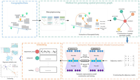
Figure 1.
Structure of semantic representation of geospatial entity categories.
3.2. Construction of Spatial Proximity Graphs of Geographical Entities
The construction of spatial proximity graph is an essential step towards achieving graph representation learning. This process involves defining the graph structure and determining the neighborhood scope.
3.2.1. Structure of the Spatial Proximity Graph
Graph is made up of nodes and edges, where nodes represent things and edges represent their relationships. We define the nodes and edges of a spatial proximity graph of geographical entity (the definition and application of graph structure are presented in Section 3.2.3).
- (1)
- Definition of Nodes
A geospatial entity is the smallest unit that records the spatial and thematic attributes of a geographic entity [50]. In this paper, geographic entities are utilized as nodes of the spatial proximity graph, with the thematic features serving as attributes of the nodes.
- (2)
- Definition of Edges
Edge is an essential entity of the graph structure that expresses the relationship between nodes. Entities with spatial proximity relationships together constitute the geographic environment. In this paper, spatial proximity is used as the basis for establishing edge associations to connect other entity nodes located within the neighborhood of a entity node.
3.2.2. Method for Determining Neighborhoods
Having a proximity relationship is a prerequisite for establishing graph node relationships (edges). This paper shifts the focus from determining whether two geospatial entity are spatially close to determining whether they are in the same spatial neighborhood, and assumes that all entity in the same spatial neighborhood have proximity relationships that can establish the association between entity nodes.
Determination of the size of the neighborhood range is a key consideration, which should be selected according to the data distribution characteristics of the study area, the needs of the target task, and domain knowledge and experience. The size of the neighborhood range can influence both the strength of the association between entity and the richness of the entity categories within the neighborhood. Association strength is defined as the correlation between the entity within the neighborhood, while richness refers to the number of geospatial entity categories within the neighborhood. According to the first law of geography, the closer the spatial distance, the stronger the correlation between the entities. However, when the range of the neighborhood is too large, the correlation between entities becomes weaker, which can make it difficult to reflect the uniqueness of the neighborhood. However, it is important to consider that a smaller neighborhood range may decrease the richness of entity categories within it, resulting in insufficient associated training entity for the model. This could potentially make it challenging for the model to accurately capture the characteristics of the neighborhood. Therefore a moderate neighborhood range (for example, 50 m) can balance association strength and category richness, thereby optimizing semantic representation. Meanwhile, by analyzing the experimental data, we found that there was a relatively dense distribution of geographical entities within a 100 m neighborhood. Therefore, we selected multiple neighborhood ranges within 200 m (10 m, 25 m, 50 m, 100 m, 200 m) for experimental analysis.
3.2.3. Method for Generating Spatial Proximity Graph
To start, a spatial proximity graph space is initialized, where represents a set of geospatial entity nodes and consists of edges that store the association relationship between entity nodes. Then, a target entity node is selected, and other neighboring entity nodes that have a proximity relationship with v are queried based on the size of the neighborhood range. The edges of entity node v can be constructed with its neighboring nodes to establish the association among them. Finally, all entity nodes are iterated through to establish associative edges of all neighboring entity to generate the spatial proximity graph.
Figure 2 shows an example of a region in Nanchang, Jiangxi Province, China. In this example, the polygon entity (osm_id is 855690625, osm_id is an identifier used to uniquely identify each object in OSM) is used as the target entity, and six neighboring entity are identified based on the neighborhood range (Table 1). Edge associations are established between each of the six entity and the target entity to construct a neighborhood relationship graph for polygon entity “855690625” (Figure 3). The complete proximity graph is created by traversing all of the entity nodes in the region (Figure 4).
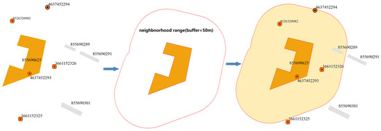
Figure 2.
According to the buffer zone, the neighboring relationship between the central and nearby entities is constructed.

Table 1.
Attribute of the example nodes.
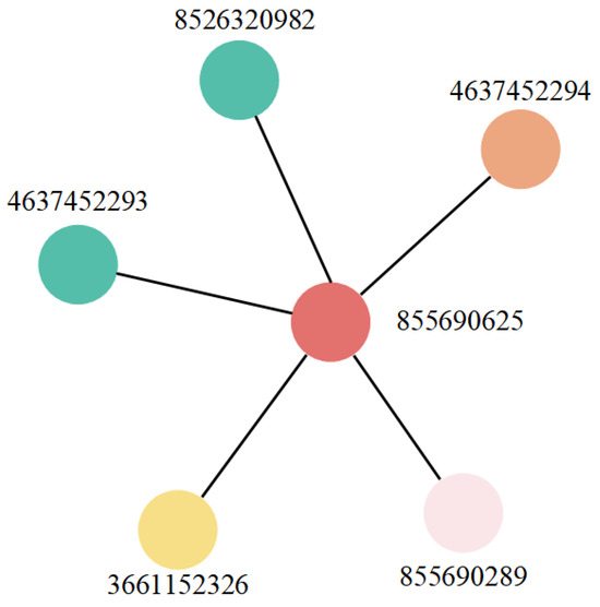
Figure 3.
Spatial proximity graph of geospatial entity (855690655).
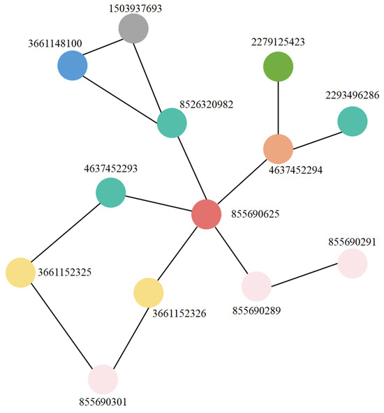
Figure 4.
Complete spatial proximity graph.
3.3. Semantic Representation Model Construction
A neighbor matrix of geospatial entity categories is constructed by employing the spatial proximity graph. After the semantic representation model is constructed, geospatial entity categories are training by SDNE. The process of constructing the semantic representation model is divided into two parts: the neighbor matrix construction of entity categories and the semantic representation model construction and training.
3.3.1. Neighborhood Matrix Construction
The entity category is an important aspect of geospatial data semantics, as it describes the data type. In this paper, a method is proposed for constructing a category neighborhood matrix. Category attributes are first extracted and then represented as matrix entities based on the one-to-one correspondence between geospatial entities and their category attributes. To calculate the neighbor strength of the relationship between entity categories, the number of correlation edges between the entity in the proximity graph is counted. The edge count value is then utilized to create the neighbor matrix, which specifies the geographical entity categories. The following are the key steps.
Firstly, the category attributes of geographical entities are treated as nodes in a spatial proximity graph, and the category attributes are utilized as matrix elements.
Secondly, for the spatial proximity graph , we randomly select the entity node (category c1) as the starting target node. Then, all the entity nodes in that have an edge association with target node are traversed. If there is an associated edge between the target node and the associated node, the total number of edges between the two is cumulatively recorded.
Next, the process is repeated for all of the entity nodes in to obtain the total number of associated edges for each entity node. The value of each element in the corresponding row and column in the adjacency matrix (Equation (1)) is determined by the total number of edges. As a result, the adjacency matrix is generated for all geospatial entity categories.
where denotes the weight of the entity category that has a proximity relationship with the central entity category j, while denotes the total number of categories in all entity categories that have a proximity relationship with j.
Finally, we obtained a category adjacency matrix that encompasses all the geographical entities of the entire experimental region.
Figure 5 shows the neighboring relationship and correlation strength of one graph node (geographic entity) in the example.
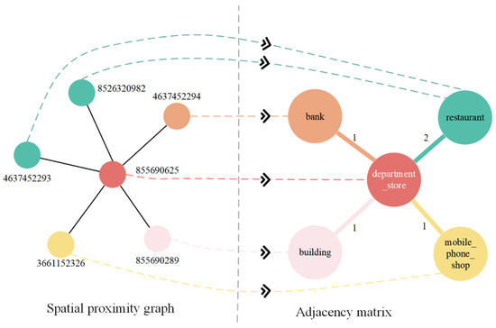
Figure 5.
A graphical representation of an adjacency matrix.
The entity categories that are spatially close to the entity category department-store are restaurant, mobile-phone-shop, building, and bank, as shown in the figure. Among them, restaurant appears most often and has the strongest neighborhood strength with department-store.
3.3.2. Entity Category Semantic Representation Model
The SDNE model is combined with the geospatial entity category adjacency matrix to construct and train the entity category semantic representation model. The training process involves capturing first- and second-order similarities and optimizing both simultaneously, resulting in final learned geospatial entity category embedding that retains both local and global structure.
First-order proximity illustrates that two geospatial entities with a proximity relationship (edge connection) have a certain degree of association. For example, there are more restaurants within the school’s neighborhood, and there is a direct edge connection between the school and the restaurant. In contrast, wetlands are less likely to occur within the school’s neighborhood, and therefore have significantly less association with the restaurant than with other entity. The first-order loss function is as follows:
represents the connection relationship between two nodes i an j, and represents the embedding vector of the node i. is the vector obtained after encoding by the encoder.
Second-order proximity illustrates the similarity of two geospatial entity that are not within each other’s neighborhood but have a similar structure. For example, two spatially separated shopping malls are similar to some degree if the composition of geospatial entity categories within their neighborhood is similar. The second-order loss function is as follows:
is the adjacency vector of node i, that is, the row value of the node in the adjacency matrix is taken. The purpose of multiplying by B here is to distinguish the difference between the values of 0 and 1, where 0 accounts for the majority and 1 only a small part. To enhance the effect of 1, it is multiplied by a value (5 is taken in the article). is the vector obtained after decoding by the decoder.
4. Experiment
The paper uses real-world datasets to conduct experiments in this part. The description of the category pair similarity comparison and region similarity tasks comes first, then the experimental region and data, and lastly, the parameter settings.
4.1. Datasets and Preprocessing
In this study, OSM data from Nanchang City is used as an experimental dataset to train feature embedding for OSM geospatial entity categories. We selected the data for which no attribute was missing. Then the dataset contains 39,926 geospatial entities across 147 entity categories.
Data preprocessing: Before we extract neighborhood entities from the dataset, we perform a series of preprocessing steps. Finally, we successfully extracted the geographic entity that met the experimental criteria. Data preprocessing primarily comprises the following four aspects: (1) Delete the isolated line feature, which is not connected to other line, surface or point entities at the boundary after data cropping; (2) Remove duplicated features; (3) Retain only the surface feature of the geographic entity which has more than one feature with multiple geometric types, and delete the feature of other geometric types. For example, the representation of some bodies of water has both a surface and a centerline, and so on; (4) Delete geographic components that describe the class’s geographical scope, such as Nanchang city, Xinjian counties. The detailed steps are shown in Figure 6.
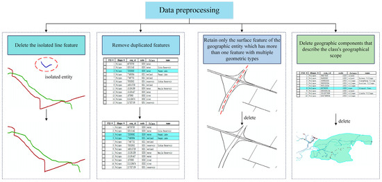
Figure 6.
The details of data processing.
After processing, the dataset contains 39,714 geospatial entities across 147 entity categories. The spatial proximity graph of entities built on this basis contains 39,714 nodes and 218,838 edges.
4.2. Experiment Setup
4.2.1. Evaluation Tasks
In this experimental study, we consider two tasks to evaluate the effectiveness of our proposed approach.
- (1)
- Category pair similarity comparison task: After training the representation learning model, similar geospatial entity categories are mapped to similar feature embeddings. The similarity between feature embeddings expresses the similarity and correlation between the semantics of the entity categories in numerical values [51,52]. and are feature embedding representations of the geographical entity classes M and N, respectively. The similarity between these two geographical entity classes will be evaluated using the cosine similarity between their embedding representations, and the model’s efficacy will be verified by comparing the similarity values produced from the standard model.
- (2)
- Regional similarity task: We use geographic entity category feature embedding in the embedding representation challenge of regions to test the feasibility of the representation learning approach for future projects.
4.2.2. Verification Program Design
- Category pair similarity comparison task
Selection of the standard model: Comparing the effectiveness of models with expert scoring is the most direct approach, but it is very time-consuming and laborious. In this paper, a semantic similarity algorithm based on dynamic weights is chosen as the standard model [8]. The algorithm introduces TF-IDF, using the value of the characteristic attributes of each geographic entity category to calculate the dynamic weight of each attribute, which reflects the importance difference of the characteristic attributes in the semantics of different geographic entity categories, and then proposes the corresponding similarity algorithm based on the different types of characteristic attributes, focusing on analyzing the decomposition of the value. The model is utilized to determine the similarity of the sample’s entity category pairings, and the calculated results are used as the standard value to evaluate the model’s validity in this study.
Selection of validation sample data: The standard model cannot be used to calculate similarity of OSM entity categories due to the absence of the corresponding ontology properties. Therefore, China’s national fundamental geographic entity categories were used as validation sample data in this paper, and the mapping was manually established between these categories and OSM feature categories. A total of 293 pairs of validation sample entity categories were obtained.
- 2.
- Regional similarity task
In this work, the region is defined as the core geographic entity’s neighborhood range, which includes the central geographic entity as well as other geographic entities within that range. This paper uses a given region A to count the frequency of each category to which each geographic entity belongs in the region, gathers the feature embedding of all geographic entity categories and forms a matrix, aggregates the feature embedding of all geographic entity categories in the region using the vector addition method, and uses the aggregated embedding as the embedding representations of the region, with the output dimensions of the region embedding set to 300. This process enables the mapping of similar regions to similar locations in the vector space. Lastly, the pairwise similarity of embedding in each region is determined using the cosine similarity method. The regions are then ordered based on their similarity, and one or more regions that are most similar to this region are output.
4.2.3. Parameter Settings
Through the experimental research in Section 5.3, the sizes of the neighborhood range are determined to be 10 m, 25 m, 50 m, 100 m, and 200 m, respectively. Finally, based on the basic guideline described in Section 3.2.2, the radius of the neighborhood is determined to be 50 m for the best balancing effect. After determining the graph structure and the neighborhood range size, the spatial proximity graph was built by using the geospatial entity as nodes and their associations with other entities in the neighborhood as edges. An adjacency matrix was built based on the attributes of the graph nodes, including the OSM entity identifiers and category. The adjacency matrix served as input to construct and train the model for semantic representation of entity categories.
The experimental environment is a 64-bit Windows operating system with an Intel Core i5 CPU processor, compiled with Python 3.7.4 and the toolkit Tensorflow 1.14.0.
The experiment included 40 training iterations (Epoch), a ReLU activation function, batch normalization after each layer, Adam as the optimizer, and first- and second-order parameters α and β set to 1 × 10⁻⁶ and 5, respectively. To reduce the negative impact of overfitting, the dense layer of the encoder model’s fully-connected neural network was chosen to use the Kernel_regularizer l1_l2 regularization to limit the weight thresholds, with l1 and l2 being 1 × 10⁻⁵ and 1 × 10⁻⁴, respectively, and the learning rate lr = 0.001.
5. Results and Discussion
In this section, we demonstrate the effectiveness of the representations in this paper and the feasibility of applying them to downstream tasks in terms of the category pair similarity comparison task and the region similarity task. The results of the tasks are discussed and analyzed, as well as the effect of different neighborhood range sizes on the entity representations.
5.1. Category Pair Similarity Comparison Task
5.1.1. Analysis of Results
Overall, the similarity calculated by using the proposed model can effectively reflect the similarity between the sample entity categories. The difference in similarity compared to the standard model is not significant. For instance, the similarity between “school–theater (cinema)”, “supermarket–hotel (restaurant)”, and “swimmingpool-open-airstadium” is approximately 0.01, demonstrating the effectiveness of the proposed model. Table 2 shows the similarity of a selection of sample entity category pairs. However, some pairs still exhibit a difference in similarity with the standard model that exceeds 0.2. There are two main scenarios:
Table 2.
Semantic similarity between pairs of classes.
- Some category pairs have slightly different ontological properties but are spatially close, e.g., “dike–gate”. They share similar neighborhood environments, and model training can yield similar feature embeddings. This is reflected in their cosine similarity, but the standard model rates similarity slightly lower. The analysis reveals that the results obtained for such cases capture both the correlation and the similarity between category pairs. This scenario cannot be directly reflected by the traditional standard model, resulting in a slight difference in the calculation results between the two.
- Some category pairs are not spatially adjacent but have similar neighborhood environments. The proposed model will lead to a slightly higher similarity score. In terms of ontological properties, the standard model provides a slightly lower similarity due to differences in some important properties, such as the “function” property between the two categories: water plant and sewage treatment plant.
The performance of the proposed model in calculating the similarity of validation sample pairs is generally consistent with the standard model. This indicates that the entity category embedding extracted by the proposed model can better reflect their semantic connotations. However, since the entity category embedding also reflects the correlation, the similarity calculation results may differ somewhat from the standard model.
5.1.2. Error Analysis
Table 3 presents the standard deviation, maximum, minimum, and median values of the error between the cosine similarity calculation results and the standard model calculation results. The standard deviation of the resulting error is small, indicating low fluctuation. This means that the difference between the similarity based on the proposed model and the similarity of the standard model is more concentrated and does not appear to be polarized. The error is mainly concentrated at a lower level, with a median value of 0.1092 and a lower upper limit.
Table 3.
The result of the overall error.
To analyze the difference between the cosine similarity calculation results and the standard model calculation results, the error values were divided into four grades: error-free (0~0.05), low error (0.05~0.2), medium error (0.2~0.3), and high error (0.3~1). Figure 7 shows the error level distribution. In general, the similarity calculation based on the proposed model is effective. The majority of error values are concentrated in the error-free and low error ranges, accounting for 26.6% and 50.5%, respectively. The medium error interval accounts for a relatively large proportion, at 17.7%. Analysis of these errors reveals that they are mainly derived from some differences in the geospatial entity categories in terms of semantic connotations while being located in similar environments. As a result, the feature embedding obtained from the proposed model will result in high similarity.
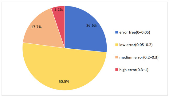
Figure 7.
The distribution of error grades is based on the similarity of our model.
5.1.3. Statistical Analysis
Pearson’s correlation coefficient is a measure of the linear consistency between two variables. A higher absolute value of the coefficient indicates a stronger consistency between the two variables, with a positive value representing a positive correlation and a negative value representing a negative correlation. In this paper, the Pearson coefficient is used to evaluate the consistency between the similarity based on the proposed model and the similarity of the standard model. The coefficient value is positive, and the higher the value, the higher the consistency between the two. The Pearson coefficient of these two similarity results is 0.7487, suggesting that the entity category embedding obtained from training the proposed model is reasonable and effective.
In this paper, the consistency of the two similarity results trends by sorting similarity values calculated by the standard model in ascending order and plotting the two results on a scatter plot, as shown in Figure 8. The figure shows that the two results are relatively close to each other in the overall trend, indirectly verifying the validity of the similarity based on the proposed model.
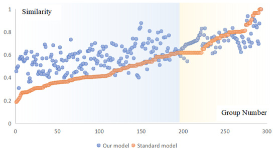
Figure 8.
Scatter plot of similarity results.
To analyze the overall consistency in more detail, this paper divides the similarity results into two parts using the 200th group as the dividing line, and it can be observed that the similarity of the entity category pairs is lower in the first part compared to the second part. After analyzing all sample pairs, it was discovered that these entity category pairs in the first part have different semantic connotations, resulting in a lower similarity calculated by the standard model. Conversely, the opposite is true in the second part. As discussed in Section 5.1.1, the feature embedding extracted from the proposed model not only measures similarity but also characterizes the strong correlation between the two. This results in the similarity of the proposed model exceeding the standard similarity value in general. The consistency of the first part is not as good as that of the second part. Entity category pairs in the second part have more similar semantic connotations, resulting in better consistency between the similarity results based on the proposed model and the standard model.
Meanwhile, the Wilcoxon symbolic rank test was conducted in this paper. It is generally used to detect whether two datasets come from a population with the same distribution. The result is shown in Table 4.
Table 4.
Wilcoxon symbolic rank test for the similarity results.
The Wilcoxon symbolic rank test was conducted on the semantic similarity calculation results of all 293 groups of data. It shows that there is a statistically significant difference in the calculation results of the two groups of models (W = 6519, p < 0.001). However, the effect size analysis indicates that the actual amplitude of the difference is relatively small (r = 0.151), and this difference only has weak practical significance (generally, it is considered that an r value between 0.1 and 0.3 is a small effect, between 0.3 and 0.5 is a medium effect, and greater than 0.5 is a large effect). To further explore the distribution characteristics of differences, the data were divided into the first part and the second part (consistent with the above text), with the 200th group as the boundary for segmented testing:
- The first part of the data: The test results showed a significant difference (W = 608, p < 0.001), but the effect size was extremely low (r = 0.030), indicating that the difference range in this interval could be ignored;
- The second part of the data: The test results did not reach the significance level (W = 1959, p = 0.386), and the difference was relatively small.
To summarize, the feature embedding extracted by this model can better express the essential characteristics of entity categories in pairs with high essential similarity, and the feature embedding extracted by this model can also better express the correlation between entities that showed low essence similarity but were similar in actual scenes. The similarity results produced are essentially compatible with traditional model similarity results, and the similarity value is slightly greater than traditional calculation results based on expert knowledge. However, unlike traditional methods that rely on domain experts to complete semantic formal expression, this method does not require expert knowledge and can swiftly express the semantics of geographical entity categories using models, which is also the algorithm’s key advantage.
5.2. Regional Similarity Task
Figure 9 and Figure 10 show the spatial structure of Region 1 and nine regions similar to Region 1, respectively. Region 1 in Figure 9 is an area with educational facilities, including various building categories, such as college, residential, sports center, pitch, library, restaurant, building, hospital, and hotel. In addition, the region also contains different types of roads, such as tertiary, secondary, and primary, and other geographical entities, such as memorials, cafes, bus stops, water, subways, drains, and rivers. Among this entity, the building category is dominant. We calculated the similarities between these nine regions and Region 1; the similarity scores from (a) to (i) were 0.98, 0.96, 0.91, 0.87, 0.81, 0.71, 0.65, 0.61, and 0.52, respectively.
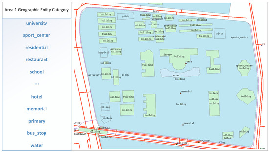
Figure 9.
Demonstration of the spatial structure of Region 1.
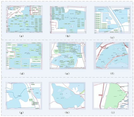
Figure 10.
Demonstration of the spatial structure of similar regions (a–i) in Region 1.
The geographic entity categories of building, subway, primary, secondary, bus stop, water, tertiary, and residential were found in each of the five similar regions (a) through (e) identified based on Figure 9. The composition of the categories in these regions is highly consistent with Region 1, and building also dominates. Similar regions (f) through (h), although slightly reduced in the number of geographical entity categories, contain main categories that are represented in Region 1 and are also dominated by educational facilities, libraries, restaurants, etc. Among them, region (g) contains the same entity categories as Region 1, such as building, college, primary, tertiary, and bus stop, with building accounting for the majority. In addition to region (g), the other two regions contain entity categories that have their corresponding categories in Region 1, although the number of buildings is smaller. In addition, there are very few categories in Region (i) that are inconsistent with Region 1; although these categories are not consistent, there are similar categories in Region 1, e.g., the canal in Region (i) is very similar to the river in Region 1.
In summary, the comparative analysis of Figure 9 and Figure 10 shows that the region-based embedding similarity can match to similar regions and not only match to regions of the same nature (e.g., all school areas, (a) to (h)) but can also capture the implied relationships between regions (i.e., regions that do not have a similar appearance performance but have a similar composition of geo-entity categories within the region, such as Region 1 and Region (i)). The analytical results further show the viability of geographic entity category feature embedding for downstream tasks.
5.3. Different Neighborhood Range Widths’ Effects on Embedding Representation
To test the influence of different neighborhood range sizes on entity representation, experiments were conducted using different neighborhood ranges to create proximity graphs. Figure 11 depicts the median, lowest, maximum, and standard deviation of the error between the similarity results of the category pairings derived by counting the different neighborhood ranges and the similarity results of the standard model. Table 5 displays the Pearson correlation coefficients for the similarity results.
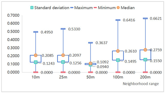
Figure 11.
Errors in similarity results.
Table 5.
Pearson correlation coefficient for the similarity results.
We discovered that when smaller or larger neighborhood ranges were used to construct the proximity graphs within the chosen 293 sets of category pairs, the standard deviation, maximum, and median of the similarity error increased significantly, as did the Pearson correlation coefficient by at least 0.1, indicating a decrease in the consistency of the similarity results and an increase in error. When the neighborhood range size is 50 m, the minimum, median, and standard deviation of the error are lower than the other ranges, with a standard deviation of 0.0940 and a median of 0.1092, showing that the error is smaller and more evenly distributed toward the median, with fewer big error values. The Pearson correlation coefficients are more consistent with the standard model, with an improvement of 0.2390 compared to the worst neighborhood range of 10 m. This shows that a suitable neighborhood range can reduce error oscillations while improving model consistency and accuracy.
Too large a neighborhood range introduces geographic entities unrelated to the central entity, increases noise, and contains too much information about entity categories that lead to excessively smooth category representations and high similarity. Conversely, too small a domain range may result in inadequate enrichment of the entity, insufficient associated entities for model training, and difficulty in obtaining an effective representation of feature embedding for differentiation. It is demonstrated that a proper neighborhood range size is crucial for the depiction of geographic entity categories, and a good domain range can be attained by a comprehensive experiment with cities and relevant tasks.
6. Conclusions
This study proposes an unsupervised method for learning the semantic representation of geospatial entity categories based on spatial proximity relations. The method constructs a spatial proximity relationship graph of geospatial entities, trains the feature embedding of geospatial entity categories, and formalizes the semantics of entity categories. Finally, the cosine similarity algorithm is used to calculate the embedding similarity between entity categories. A comparison experiment is then conducted with the similarity results of the standard model. The experimental results show that the proposed model better reflects the similarity and correlation of geospatial entity category pairs. This demonstrates the effectiveness of the proposed model and provides a new way of thinking for the unsupervised training of the semantic representation of geospatial entity categories. Furthermore, when analyzing category pairs that are significantly different from the standard model, it is found that our model has certain advantages in capturing specific types of geographic semantic relations (such as spatial co-occurrence). However, the validity of the proposed model has only been confirmed in this paper. New ideas can be provided for training semantic representations of geographic entity categories in an unsupervised way. In future work, the following should be considered: (1) Geographic entity category descriptions contain characteristic information of the categories themselves in addition to the semantic relations between the categories; thus, finding ways to effectively access the knowledge representation of the entity categories and combining them with the semantic relations can better improve the quality of the formal representation of geographic entity categories. (2) Feature embedding can also serve as input features for deep neural network training datasets. (3) One can utilize the model to capture specific types of geographic semantic relationships and conduct research in areas such as spatial co-occurrence patterns. In this research, we merely established their validity; in future work, we will aim to add other text and spatiotemporal data, for example, to expand the informative richness of the embedding representation, and then use the embedding for other downstream tasks such as prediction and analysis.
Author Contributions
Conceptualization, Yongbin Tan; methodology, Yongbin Tan and Lingling Gao; software, Rongfeng Cai; validation, Zhonghai Yu; formal analysis, Xin Li; data curation, Zhonghai Yu; writing—original draft preparation, Rongfeng Cai and Hong Wang; writing—review and editing, Hong Wang; visualization, Xin Li. All authors have read and agreed to the published version of the manuscript.
Funding
This research was funded by National Natural Science Foundation of China, grant number 42361067, National Natural Science Foundation of China, grant number 42261078, the East China University of Technology Foundation, grant number No. DHYC-202411, Shandong Provincial Natural Science Foundation, grant number ZR2024QD123.
Data Availability Statement
The original data presented in the study are openly available in https://openstreetmap.org.
Conflicts of Interest
Author Rongfeng Cai was employed by the company China Rare Earth (Liangshan) Co., Ltd. The remaining authors declare that the research was conducted in the absence of any commercial or financial relationships that could be construed as a potential conflict of interest.
References
- Duan, X. Research on Ontology Alignment Method and Optimization Algorithm Based on Deep Learning; Chongqing Normal University: Chongqing, China, 2020. [Google Scholar]
- Zhao, Y.; Sun, Q.; Liu, X.; Cheng, M.; Yu, T.; Li, Y. Geographical entity-oriented semantic similarity measurement method and its application in road matching. Geomat. Inf. Sci. Wuhan Univ. 2020, 45, 728–735. [Google Scholar]
- Ling, Z.; Li, R.; Wu, H.; Li, J.; Gui, Z. Semantic-driven construction of geographic entity association network and knowledge service. Acta Geod. Cartogr. Sin. 2023, 52, 478. [Google Scholar]
- Li, W.; Zhang, Y.; Pan, L. Ontology concept update method based on semantic similarity. Comput. Appl. Softw. 2018, 35, 15–20. [Google Scholar]
- Wang, L.; Zhang, F.; Du, Z.; Chen, Y.; Zhang, C.; Liu, R. A hybrid semantic similarity measurement for geospatial entities. Microprocess. Microsyst. 2021, 80, 103526. [Google Scholar] [CrossRef]
- Zhao, H.; Zhu, Y.; Yang, H.; Luo, K. The semantic relevancy computation model on essential features of geospatial data. Geogr. Res 2016, 35, 58–70. [Google Scholar]
- Zhu, G.; Iglesias, C.A. Computing semantic similarity of concepts in knowledge graphs. IEEE Trans. Knowl. Data Eng. 2016, 29, 72–85. [Google Scholar] [CrossRef]
- Yongbin, T.A.N.; Lingling, G.A.O.; Lin, L.I.; Penggen, C.H.E.N.G.; Hong, W.A.N.G.; Xiaolong, L.I.; Cheng, C.H.E.N. A dynamic weighted model for semantic similarity measurement between geographic feature categories. Acta Geod. Cartogr. Sin. 2023, 52, 843. [Google Scholar]
- Li, L.; Zhu, H.H.; Wang, H.; Li, D.R. Semantic analyses of the fundamental geographic Information based on formal ontology—Exemplifying hydrological category. Acta Geod. Cartogr. Sin. 2008, 37, 230–235. [Google Scholar]
- Li, H.; Zhai, L.; Zhu, H. Semantic similarities calculative modeling for geospatial entity classes based on ontology. Sci. Surv. Mapp. 2009, 34, 12–14. [Google Scholar]
- Tan, Y.; Li, L.; Wang, W.; Yu, Z.; Zhang, Z.; Mao, K.; Xu, Y. Semantic similarity measurement model between fundamental geographic information concepts based on ontological property. Acta Geod. Cartogr. Sin. 2013, 42, 782. [Google Scholar]
- Zhang, D.; Yin, J.; Zhu, X.; Zhang, C. Network representation learning: A survey. IEEE Trans. Big Data 2018, 6, 3–28. [Google Scholar] [CrossRef]
- Bengio, Y.; Courville, A.; Vincent, P. Representation learning: A review and new perspectives. IEEE Trans. Pattern Anal. Mach. Intell. 2013, 35, 1798–1828. [Google Scholar] [CrossRef] [PubMed]
- Perozzi, B.; Al-Rfou, R.; Skiena, S. Deepwalk: Online learning of social representations. In Proceedings of the 20th ACM SIGKDD International Conference on Knowledge Discovery and Data Mining, New York, NY, USA, 24–27 August 2014; pp. 701–710. [Google Scholar]
- Narayanan, A.; Chandramohan, M.; Venkatesan, R.; Chen, L.; Liu, Y.; Jaiswal, S. graph2vec: Learning distributed representations of graphs. arXiv 2017, arXiv:1707.05005. [Google Scholar]
- Grover, A.; Leskovec, J. node2vec: Scalable feature learning for networks. In Proceedings of the 22nd ACM SIGKDD International Conference on Knowledge Discovery and Data Mining, New York, NY, USA, 13–17 August 2016; pp. 855–864. [Google Scholar]
- Wang, D.; Cui, P.; Zhu, W. Structural deep network embedding. In Proceedings of the 22nd ACM SIGKDD International Conference on Knowledge Discovery and Data Mining, San Francisco, CA, USA, 13–17 August 2016; pp. 1225–1234. [Google Scholar]
- Tang, J.; Qu, M.; Wang, M.; Zhang, M.; Yan, J.; Mei, Q. Line: Large-scale information network embedding. In Proceedings of the 24th International Conference on World Wide Web, Florence, Italy, 18–22 May 2015; pp. 1067–1077. [Google Scholar]
- Cao, S.; Lu, W.; Xu, Q. Grarep: Learning graph representations with global structural information. In Proceedings of the 24th ACM International on Conference on Information and Knowledge Management, Melbourne, Australia, 18–23 October 2015; pp. 891–900. [Google Scholar]
- Belkin, M.; Niyogi, P. Laplacian eigenmaps for dimensionality reduction and data representation. Neural Comput. 2003, 15, 1373–1396. [Google Scholar] [CrossRef]
- Jones, C.B.; Ware, M.J. Nearest neighbor search for linear and polygonal objects with constrained triangulations. In Proceedings of the 8th International Symposium on Spatial Data Handling, Vancouver, BC, Canada, 11–15 July 1998; pp. 13–21. [Google Scholar]
- Yan, C.; Liu, X.; Li, A. The representation and application of spatial neighborhood. J. Spatio-Temporal Inf. 2018, 25, 18–22. [Google Scholar]
- Zhu, A.; Lv, G.; Zhou, C.; Qin, C. Geographic similarity: Third law of geography? J. Geo-Inf. Sci. 2020, 22, 673–679. [Google Scholar]
- Song, Y. Geographically optimal similarity. Math. Geosci. 2023, 55, 295–320. [Google Scholar] [CrossRef]
- Zhu, A.; Turner, M. How is the Third Law of Geography different? Ann. GIS 2022, 28, 57–67. [Google Scholar] [CrossRef]
- Zhu, A.X.; Lu, G.; Liu, J.; Qin, C.-Z.; Zhou, C. Spatial prediction based on third law of geography. Ann. GIS 2018, 24, 225–240. [Google Scholar] [CrossRef]
- Jiao, Z.; Tao, R. Geographical Gaussian Process Regression: A Spatial Machine-Learning Model Based on Spatial Similarity. Geogr. Anal. 2025. [Google Scholar] [CrossRef]
- Dhyani, D.; Ng, W.K.; Bhowmick, S.S. A survey of web metrics. ACM Comput. Surv. (CSUR) 2002, 34, 469–503. [Google Scholar] [CrossRef]
- Hamming, R.W. Error detecting and error correcting codes. Bell Syst. Tech. J. 1950, 29, 147–160. [Google Scholar] [CrossRef]
- Zhao, Y. Research on Key Technology of Semantic Consistency Processing for Multi-Sources Vector Data; Information Engineering University: Zhengzhou, China, 2021. [Google Scholar]
- Xu, Z.; Zhu, Y.; Song, J.; Sun, K.; Wang, S. Word embedding-based method for entity category alignment of geographic knowledge base. Inf. Sci. 2021, 23, 1372–1381. [Google Scholar]
- Salton, G.; Wong, A.; Yang, C. A vector space model for automatic indexing. Commun. ACM 1975, 18, 613–620. [Google Scholar] [CrossRef]
- Zhuang, B.; Liu, L.; Shen, C.; Reid, I. Towards context-aware interaction recognition for visual relationship detection. In Proceedings of the 2017 IEEE International Conference on Computer Vision (ICCV), Venice, Italy, 22–29 October 2017; pp. 589–598. [Google Scholar]
- Barkan, O.; Koenigstein, N. Item2vec: Neural item embedding for collaborative filtering. In Proceedings of the 2016 IEEE 26th International Workshop on Machine Learning for Signal Processing (MLSP), Vietri sul Mare, Italy, 13–16 September 2016; pp. 1–6. [Google Scholar]
- Wu, S.; Roberts, K.; Datta, S.; Du, J.; Ji, Z.; Si, Y.; Soni, S.; Wang, Q.; Wei, Q.; Xiang, Y.; et al. Deep learning in clinical natural language processing: A methodical review. J. Am. Med. Inform. Assoc. 2020, 27, 457–470. [Google Scholar] [CrossRef]
- Bordes, A.; Usunier, N.; Garcia-Duran, A.; Weston, J.; Yakhnenko, O. Translating embeddings for modeling multi-relational data. In Proceedings of the 27th International Conference on Neural Information Processing Systems, Lake Tahoe, NV, USA, 5–10 December 2013; p. 26. [Google Scholar]
- Wang, Z.; Zhang, J.; Feng, J.; Chen, Z. Knowledge graph embedding by translating on hyperplanes. In Proceedings of the Twenty-Eighth AAAI Conference on Artificial Intelligence, Québec City, QC, Canada, 27–31 July 2014. [Google Scholar]
- Lin, Y.; Liu, Z.; Sun, M.; Liu, Y.; Zhu, X. Learning entity and relation embeddings for knowledge graph completion. In Proceedings of the Twenty-Ninth AAAI Conference on Artificial Intelligence, Austin, TX, USA, 25–30 January 2015. [Google Scholar]
- Ji, G.; He, S.; Xu, L.; Liu, K.; Zhao, J. Knowledge graph embedding via dynamic mapping matrix. In Proceedings of the 53rd Annual Meeting of the Association for Computational Linguistics and the 7th International Joint Conference on Natural Language Processing (Volume 1: Long Papers); Association for Computational Linguistics: Beijing, China, 2015; pp. 687–696. [Google Scholar]
- Tu, C.; Yang, C.; Liu, Z.; Sun, M. Network representation learning: An overview. Sci. Sin. Informationis 1998, 43, 1681. [Google Scholar]
- Kipf, T.N.; Welling, M. Semi-supervised classification with graph convolutional networks. arXiv 2016, arXiv:1609.02907. [Google Scholar]
- Veličković, P.; Cucurull, G.; Casanova, A.; Romero, A.; Liò, P.; Bengio, Y. Graph attention networks. arXiv 2017, arXiv:1710.10903. [Google Scholar]
- Zhang, C.; Zhang, K.; Yuan, Q.; Peng, H.; Zheng, Y.; Hanratty, T.; Wang, S.; Han, J. Regions, periods, activities: Uncovering urban dynamics via cross-modal representation learning. In Proceedings of the 26th International Conference on World Wide Web, Perth, Australia, 3–7 April 2017; pp. 361–370. [Google Scholar]
- Zhao, P.; Han, J.; Sun, Y. P-rank: A comprehensive structural similarity measure over information networks. In Proceedings of the 18th ACM Conference on Information and Knowledge Management, Hong Kong, China, 2–6 November 2009; pp. 553–562. [Google Scholar]
- Fu, Y.; Wang, P.; Du, J.; Wu, L.; Li, X. Efficient region embedding with multi-view spatial networks: A perspective of locality-constrained spatial autocorrelations. In Proceedings of the AAAI Conference on Artificial Intelligence, Honolulu, HI, USA, 27 January–1 February 2019; pp. 906–913. [Google Scholar]
- Liu, K.; Gao, S.; Qiu, P.; Liu, X.; Yan, B.; Lu, F. Road2vec: Measuring traffic interactions in urban road system from massive travel routes. ISPRS Int. J. Geo-Inf. 2017, 6, 321. [Google Scholar] [CrossRef]
- Jia, H.; Chen, M.; Huang, W.; Zhao, K.; Gong, Y. Learning hierarchy-enhanced POI category representations using disentangled mobility sequences. In Proceedings of the Thirty-Third International Joint Conference on Artificial Intelligence, Jeju, Republic of Korea, 3–9 August 2024; pp. 2090–2098. [Google Scholar]
- Li, Y.; Chen, T.; Luo, Y.; Yin, H.; Huang, Z. Discovering collaborative signals for next POI recommendation with iterative Seq2Graph augmentation. arXiv 2021, arXiv:2106.15814. [Google Scholar]
- Wang, M.X.; Lee, W.C.; Fu, T.Y. On representation learning for road networks. ACM Trans. Intell. Syst. Technol. (TIST) 2020, 12, 1–27. [Google Scholar] [CrossRef]
- Wang, H. Application study on basic geographic elements in big data environment. Geomat. Spat. Inf. Technol. 2015, 38, 191–193. [Google Scholar]
- Budanitsky, A.; Hirst, G. Evaluating wordnet-based measures of lexical semantic relatedness. Comput. Linguist. 2006, 32, 13–47. [Google Scholar] [CrossRef]
- Resnik, P. Using information content to evaluate semantic similarity in a taxonomy. arXiv 1995, arXiv:cmp-lg/9511007. [Google Scholar]
Disclaimer/Publisher’s Note: The statements, opinions and data contained in all publications are solely those of the individual author(s) and contributor(s) and not of MDPI and/or the editor(s). MDPI and/or the editor(s) disclaim responsibility for any injury to people or property resulting from any ideas, methods, instructions or products referred to in the content. |
© 2025 by the authors. Published by MDPI on behalf of the International Society for Photogrammetry and Remote Sensing. Licensee MDPI, Basel, Switzerland. This article is an open access article distributed under the terms and conditions of the Creative Commons Attribution (CC BY) license (https://creativecommons.org/licenses/by/4.0/).