Article

R-MLGTI: A Grid- and R-Tree-Based Hybrid Index for Unevenly Distributed Spatial Data

1
School of Computer Science, China University of Geosciences, Wuhan 430074, China
2
Engineering Research Center of Natural Resource Information Management and Digital Twin Engineering Software, Ministery of Education, Wuhan 430074, China
*
Author to whom correspondence should be addressed.
ISPRS Int. J. Geo-Inf. 2025, 14(6), 231; https://doi.org/10.3390/ijgi14060231
Submission received: 7 February 2025 / Revised: 3 June 2025 / Accepted: 6 June 2025 / Published: 12 June 2025

Abstract

In recent years, with the development of sensor technology, the volume of spatial data has grown exponentially. However, this data is often unevenly distributed, and traditional indexing methods cannot predict the overall data distribution when data are continuously inserted into the database. This makes them inefficient for indexing large-scale, unevenly distributed spatial data. This paper proposes a hybrid indexing method based on the grid-indexing and R-tree methods, called R-MLGTI (R-Multi-Level Grid–Tree Index). The method first divides the two-dimensional space using the Z-curve to form multiple sub-grid regions. When incrementally inserting data, R-MLGTI calculates the grid encoding of the data and computes the c ( G ) of the corresponding grid G to measure the sparsity or density within the grid region, where c ( G ) is a metric that quantifies the data density within grid G. All data in sparse grids are indexed by R-trees associated with grid encodings. In dense grid areas, a finer-grained space-filling curve is recursively applied for further spatial division. This process forms multiple sub-grids until the data within all sub-grids becomes sparse, at which point the original data is re-indexed according to the sparse grids. Finally, this paper presents a prototype system of the in-memory R-MLGTI and conducts benchmark tests for incremental data import and range queries. The incremental data insertion performance of R-MLGTI is lower than that of the grid-indexing and R-tree methods; however, on various unevenly distributed simulated datasets, the average query time for different query regions in R-MLGTI is about 6.49% faster than that of the grid-indexing method and about 51.78% faster than that of the R-tree method. On a real dataset, Landsat 7 EMT, which contains 2,585,203 records, the average query time for various query ranges is 61.39% faster than that of the grid-indexing method and 17.01% faster than that of the R-tree method. Experiments show that R-MLGTI performs better than the traditional R-tree and grid-indexing methods in large-scale, unevenly distributed spatial data query requests.

1. Introduction

With the development of information and sensor technologies, the methods and techniques for acquiring spatial data are continuously evolving and innovating. Supported by advanced technologies such as Geographic Information Systems (GIS), remote sensing, and Global Positioning Systems (GPSs), the speed of global spatial data collection and updates has significantly accelerated, resulting in an explosive growth in data volumes. These data play an important role in monitoring land-use changes, tracking environmental dynamics, assessing the carbon cycle, and supporting sustainable development [1,2,3,4,5]. However, when dealing with these massive and complex spatial datasets, we often lack prior knowledge of the data’s overall structure or distribution patterns. This uncertainty creates challenges as the data is incrementally ingested into storage systems. Traditional indexing methods face significant bottlenecks under these conditions; for instance, grid-based and spatial-partitioning methods cannot adapt their structures to accommodate dynamic changes in data distribution, while the R-tree method, although capable of dynamic adjustment, suffers from decreased efficiency when managing large-scale datasets. Consequently, in the era of big data, achieving efficient retrieval of spatial data with dynamically evolving distributions has become a critical issue that demands urgent attention.
Spatial data can be divided into spatial vector data and spatial raster data. Vector data represents geographic entities through geometric objects such as points, lines, or polygons [6,7]. Traditional surveying data, location-based data (such as GPS data), geotagged information generated by social media, and real-time location data collected by IoT devices are examples of spatial data. These types of data are highly structured, with clear geometric shapes and topological relationships, enabling a precise description of the forms and locations of geographic features. Raster data, on the other hand, is a data type that divides and represents spatial regions based on pixels. Each pixel represents a fixed area and stores attribute values related to that region. For example, remote sensing imagery is a typical form of raster data, obtained through satellite or aerial images, and can support land-use classification, environmental change monitoring, and other applications.
Spatial indexing is widely used to organize data and optimize queries, typically utilizing tree-based and grid-based indexing methods [8]. Tree-based indexing offers good dynamic characteristics and spatial locality, supporting dynamic data insertion, deletion, and updates. However, a single tree-based index, such as an R-tree, which uses MBRs (minimum bounding rectangles) as indexing units, suffers from increased overlap of non-leaf node MBRs as the data volume grows. This overlap leads to redundant storage and unnecessary computations, ultimately reducing query performance. Grid-based indexing, when combined with space-filling curves, enhances query efficiency through dimensionality reduction. However, when objects span multiple grids, it can result in data redundancy, thus reducing indexing efficiency [8]. In large-scale spatial data, especially when the data distribution is uneven, a single grid structure with fixed grid levels cannot effectively handle data-dense regions, causing a significant decline in query efficiency. When data is highly concentrated within a specific grid cell, the query process must handle an excessive number of objects, which increases computational load and negatively affects indexing performance.
In this paper, we propose a hybrid indexing method based on the grid-indexing and R-tree methods called R-MLGTI (R-Multi-Level Grid–Tree Index). This method divides the space using a multi-level dynamic grid-partitioning approach and employs an R-tree for indexing the spatial data within each grid cell. On one hand, dynamic grid partitioning adapts to ongoing data insertions, ensuring the rationality of the partitions. On the other hand, when dealing with data-dense grid cells, the presence of an R-tree eliminates the need to directly traverse all data within the grid cell. Range queries using the R-tree allow for faster filtering of target data. Furthermore, grid partitioning enables parallel operations of the R-tree across multiple cells, significantly improving retrieval efficiency. In addition, based on the proposed indexing method, a corresponding storage structure is designed, and the hybrid indexing method is implemented in memory. A performance comparison of the indexing efficiency was conducted between the R-tree and grid-indexing structures based on the Z-curve. The results confirm that the hybrid indexing method proposed in this paper performs better when handling large-scale spatial data, especially data with an uneven distribution.
The rest of this paper is organized as follows. Section 2 introduces the grid-based spatial data indexing and tree-based spatial data indexing methods. Section 3 details the structure and implementation of R-MLGTI. Section 4 presents the experiments and analyzes the results, and Section 6 concludes this paper.

2. Related Works

Currently, research on spatial data indexing structures can be classified into two categories: tree-based structures and grid-based structures.

2.1. Spatial Indexing Based on Tree Structures

Tree-based index structures typically use the MBR of spatial objects as the indexed entity. The main concept behind this method is to approximate spatial objects using spatial polygons, which can be represented by approximate polygons. Then, approximate polygons are constructed based on the organization of the index structure [9]. Research on tree structures has been extensive. In 1984, Guttman et al. introduced the concept of the R-tree [10], which is an extension of the B+ tree. The R-tree is designed to better address issues related to data storage and query processing.
The R-tree is a hierarchical spatial-indexing method, with its structure illustrated in Figure 1. It is primarily used for organizing and querying high-dimensional data. By encapsulating the spatial objects within an MBR, the R-tree recursively constructs a tree structure. The leaf nodes store the MBRs of actual data objects, while non-leaf nodes store the MBRs of their child nodes, which represent the coverage of their subtrees. During query processing, the R-tree filters intersecting MBRs layer by layer, effectively reducing the search space. This makes it well-suited for handling complex operations such as range queries and nearest-neighbor queries. Its dynamic properties support data insertion, deletion, and updates while maintaining tree balance, ensuring query efficiency.
The R-tree performs well in spatial data indexing; however, when data distribution is uneven, the continuous insertion of data can lead to significant overlap and coverage among MBRs, resulting in a noticeable decline in indexing performance and query efficiency [11]. Moreover, operations such as data insertion and deletion may cause frequent tree restructuring. For instance, when inserting a new object, if the current leaf node is full, the R-tree requires node splitting, which can impact the tree’s balance and subsequently degrade query performance.
Sellis et al. [12] proposed the R+-tree, a variant of the R-tree, which effectively addresses the issue of significant overlap among intermediate nodes in the R-tree, thereby improving the efficiency of spatial data queries. The R*-tree, designed by Guttman in 1990, applies a node optimization strategy by enforcing node reinsertion. This approach enhances space utilization and reduces the frequency of node splits. In 1994, Kamel and Faloutsos proposed the Hilbert R-tree [13], a structure that maps multidimensional spatial data into one-dimensional Hilbert values to enhance the spatial locality of R-trees, thereby improving query performance. Although this approach effectively mitigates the overlap and coverage issues commonly found in traditional R-trees when handling high-dimensional data, it suffers from high re-encoding overhead during dynamic updates due to the global nature of space-filling curves, which impacts overall efficiency.

2.2. Spatial Indexing Based on Grids and Spatial Partitioning

The grid-based indexing method is based on the idea of dividing a spatial region into grids of uniform or varying sizes, with each grid containing multiple spatial objects [14,15,16]. When querying target data, the grid-based method first identifies the grid cells covered by the query region and then quickly retrieves the spatial objects that meet the query conditions from these cells. Essentially, the grid represents a method of spatial partitioning. Grid indexing can be combined with space-filling curves, which can be regarded as a hashing approach for a two-dimensional space [17]. The grid divides data into m × n small blocks, while the space-filling curve maps the two-dimensional data of these m × n cells to a one-dimensional storage space. After mapping to a one-dimensional space, an index can be constructed by calculating the corresponding index values of the spatial objects, thereby marking their spatial positions. Common space-filling curves include the Hilbert curve, Z-order curve, Peano curve, and Gray code, among others [18]. By pre-partitioning the space, grid indexing eliminates the need to update the index when moving objects remain within the same spatial cell. When handling high-frequency concurrent operations, grid-based spatial-partitioning indices significantly outperform the R-tree family of indices [19].
Huang et al. [20] systematically described the grid structure and introduced the concept of multi-level grids to address the issue of the uneven distribution of two-dimensional spatial data. In 2016, Tang et al. [21] proposed an algorithm that divides a space into grids and achieves rapid spatial data partitioning using Z-order curves. Xu et al. [22] proposed a nearest-neighbor query algorithm based on space-filling-curve grid partitioning. This algorithm leverages the dimensionality-reducing property of space-filling curves and the clustering characteristics of data, linearly sorting points within the grid. By accessing points within the query point’s grid and its neighboring grids, it efficiently finds the nearest neighbors. GeoHash maps geographical locations (e.g., latitude and longitude coordinates) to a one-dimensional string, recursively dividing the space into binary grids while alternately encoding the location information of the latitude and longitude; this results in a compact GeoHash string. GeoHash exhibits spatial continuity and hierarchy, enabling the efficient indexing, querying, and storage of spatial data.
The research team led by Cheng Chengqi from Peking University proposed the GeoSOT (Geographic coordinate Subdividing grid with One-dimensional integral coding on Tree) method, which uses a one-dimensional integer array for global latitude and longitude partitioning [23,24,25]. This method has been widely applied in spatial data indexing and retrieval [26,27,28]. Tong et al. [29] proposed the Multi-Scale Time-Partitioning and Integer-Coding (MTIC) method. By using this method to index the temporal information of objects, efficient multi-scale querying can be achieved. GeoSOT-ST extends the GeoSOT spatial-partitioning scheme to the temporal dimension, forming a global spatiotemporal subdivision scheme [30,31].
Guo [32] and Huang [33] combined the Hilbert curve with GeoHash and GeoSOT, respectively, to perform queries on spatial objects. Wu [34] proposed a spatiotemporal indexing method based on GeoHash grids, utilizing Hilbert-curve encoding. Wang [35] designed a subspace-partitioning algorithm based on the concept of secondary indexing, using the Hilbert curve to support multidimensional queries. However, most of these methods do not address the issue of inefficient range queries in the case of data imbalance.
Since grid-based indexing typically partitions the space statically, the indexed objects and query regions often span multiple grid cells. When the query region spans multiple grid cells, all the data within the covered grid cells must be scanned. When the data volume within the grid cells is large, indexing efficiency may decrease significantly, as shown in Figure 2b. Although the final query results only include M5 and M6, since the query box spans four grids (00, 01, 02, and 03), all data within these four spaces will be scanned.

2.3. Multi-Structure Hybrid Indexing Methods

Yang and Huang [36] proposed a hybrid indexing structure based on an extended quadtree and a 3D R-tree, which is applied to the management and visualization of large-scale, high-density ground point cloud data. Gong et al. [37] introduced an extended 3D R-tree indexing method that considers multiple levels of detail. This method establishes a balanced structure for the indices through global optimization and 3D clustering analysis and designs a node selection algorithm. The algorithm employs a node-splitting method based on the k-medoids clustering algorithm, ensuring uniform node size, regular shape, and low overlap.
Sharifzadeh and Shahabi [38] proposed the VoR-R-tree hybrid indexing structure, which integrates Voronoi diagrams with an R-tree. By utilizing the neighborhood search characteristics of Voronoi diagrams, this structure reduces the R-tree overlapping space, thereby improving the efficiency of nearest-neighbor queries. Gong et al. [39] introduced an efficient point cloud data management method based on octrees and a 3D R-tree, aimed at addressing large-scale data management challenges. However, when the number of octrees becomes excessive, it may lead to a waste of storage space.
Song et al. [40] proposed a hybrid tree spatial-indexing structure for 3D GIS, combining octrees and an R-tree to overcome the performance bottleneck of a single spatial-indexing structure in large-scale data. However, the R-tree still faces issues with overlapping intermediate nodes, and multi-path queries continue to limit improvements in indexing performance. Liu et al. [41] further proposed a hybrid indexing method based on a 3D grid–R-tree. This method partially addresses the issue of uneven data distribution, but due to the arbitrary parameter-based division of the single-layer grid, which lacks rationality, it may still lead to data redundancy and multi-path query problems in the R-tree, thus limiting indexing performance.
Liu [42] proposed a spatial-indexing method based on the tile quadtree (T-Qtree), combined with the Distributed Data Computing (DisDC) model. Through the TQTG and TQTBV algorithms, it achieves rapid indexing and efficient visualization of large-scale vector data, significantly improving construction speed and memory efficiency. However, this method primarily optimizes the visualization of large-scale vector data, and its adaptability to higher-level data and other spatial analysis tasks remains to be verified. Zhang [43] proposed a hybrid spatial index structure based on the quadtree and the R-tree, which optimizes the spatial retrieval efficiency of 3D ENC data. By using the smallest minimum bounding box and classification retrieval methods, it reduces the overlap of index nodes and improves the rendering speed and management efficiency of 3D ENC data.

3. Method

3.1. Data Applicable to Indexing

Geospatial data is information related to specific locations on the Earth’s surface. Formally speaking, any data that can be referenced by geographical coordinates, such as latitude and longitude, or spatial identifiers, such as region names or grid cells, is regarded as geospatial data. The typical forms of geospatial data include point data, line data, and polygon data, all of which can have their minimum bounding rectangles (MBRs) calculated. Consider a two-dimensional geospatial object defined by a set of n vertices, where the coordinates of the vertices are given by
P = { ( x 1 , y 1 ) , ( x 2 , y 2 ) , , ( x n , y n ) }
The corresponding minimum bounding rectangle (MBR) can therefore be represented by the following intervals:
M B R ( P ) = [ x min , x max ] × [ y min , y max ]
where
x min = min 1 i n x i , x max = max 1 i n x i y min = min 1 i n y i , y max = max 1 i n y i
The R-MLGTI indexing structure proposed in this paper is specifically designed for geospatial data objects whose minimum bounding rectangles (MBRs) can be explicitly computed. The MBR serves as the fundamental indexing unit in R-MLGTI. During the indexing process, R-MLGTI records the MBR of each target geospatial object along with its unique data identifier, thereby enabling efficient management and control of the corresponding data entities.

3.2. R-MLGTI Index Structure

The multi-level grid-partitioning R-tree index (R-MLGTI) model proposed in this paper combines the advantages of grid partitioning and tree indexing. R-MLGTI first dynamically partitions the space using grids of different levels based on the current data distribution and then uses an R-tree to index and manage the data within each partition cell.
Whether it is spatial vector data or spatial raster data, their corresponding MBRs can be obtained. Therefore, the MBR is the minimum indexing unit of R-MLGTI. This allows R-MLGTI to manage most non-uniformly distributed spatial data.

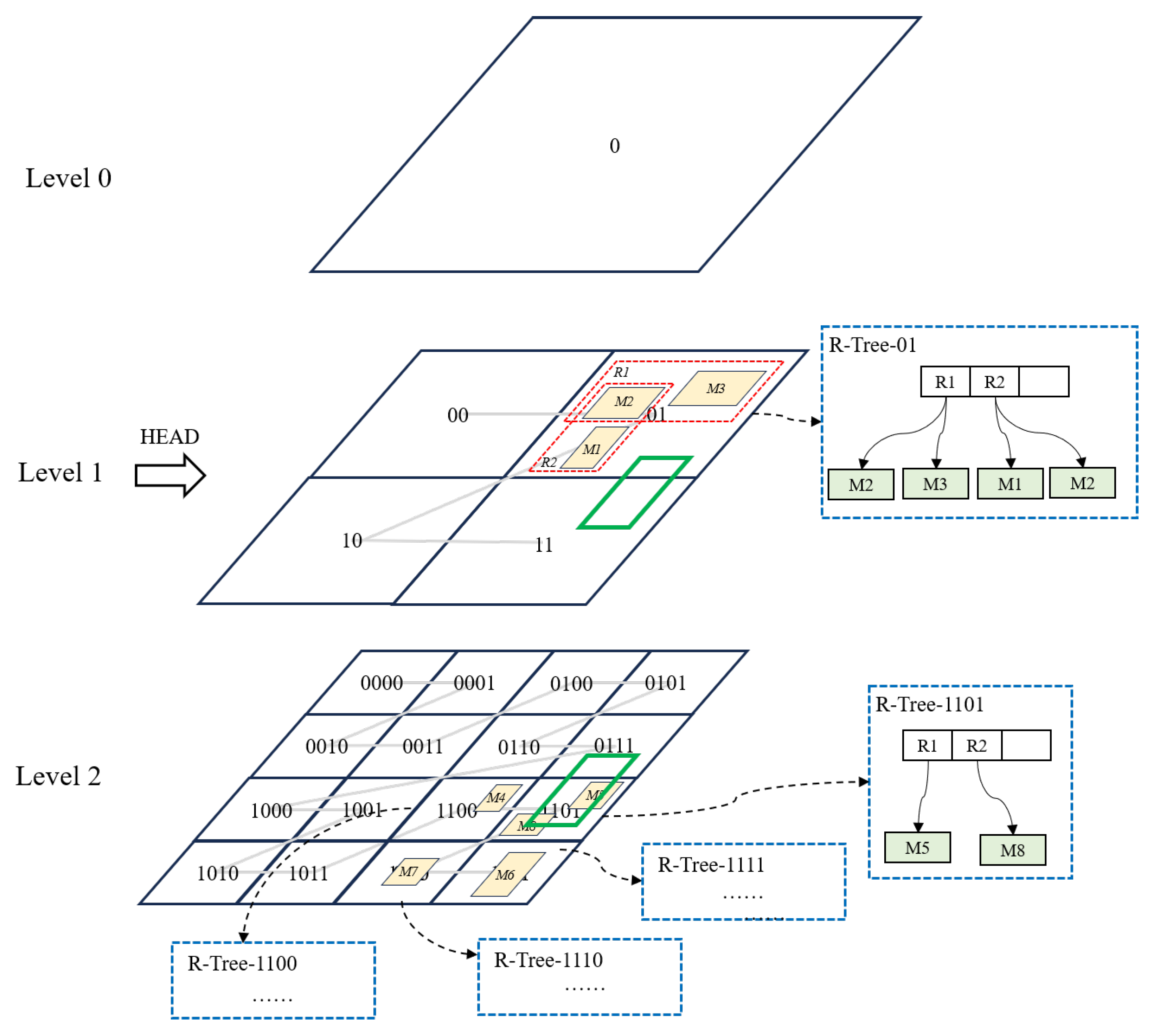
3.2.1. Grid and R-Tree

Due to its regular structural properties, the Z-order curve often offers higher efficiency in quickly locating query windows and performing range-based code filtering [44]. Therefore, we adopt the Z-order curve to partition the global geographic space, and each cell is encoded based on the chosen partition level, as illustrated in Figure 3. In a second-order Z-order curve, both the longitude and latitude are each evenly divided into two intervals, resulting in four subspaces encoded as 00, 01, 10, and 11. A third-order Z-order curve further subdivides each axis into two intervals, yielding 16 subspaces with codes ranging from 0000 to 1111. The third-order encoding can be interpreted as a refinement of the second-order subspaces. Specifically, subspaces sharing a common prefix in the higher-order encoding correspond to the same region at a coarser granularity. For example, the region encoded as 11 in the second-order partition corresponds to four subspaces—1100, 1101, 1110, and 1111—in the third-order partition, all of which share the common prefix 11.
After determining the grid space partitioning, R-trees are used to index the data within each grid cell. The diagram in Figure 3 illustrates the data distribution after partitioning the space based on the second-order Z-curve. M 1 , M 2 , and  M 3 are all located within cell region 01, and their spatial information is stored in the R-tree associated with this cell. Similarly, the spatial information of M 5 and M 8 is recorded by the R-tree corresponding to 1101.
From a data structure perspective, the entire index is composed of a forest of R-trees, where the entry points of the forest can be viewed as the grid partitions created by the Z-curve. From a functional perspective, the grid serves as a partitioning mechanism, effectively subdividing the large space into smaller datasets. This helps mitigate the issue of excessive overlapping of intermediate MBRs in a single R-tree due to the large volume of data. On the other hand, partitioning the space using grids inherently offers parallelism advantages, as the R-tree within each grid cell can operate independently without interference.
The indexing workflow is illustrated in Figure 4, where the green region denotes the query window. During the query process, we first locate the grid at the H E A D level, which in this case corresponds to L e v e l 2 . At this level, the query window intersects with two target grids: 01 and 11. The 01 grid contains relatively sparse data, and therefore the query is directly processed using the R-tree index associated with this grid, denoted as R T r e e 01 , yielding result R 1 . In contrast, the 11 grid contains denser data and has been delegated to a finer-grained level, L e v e l 3 for further indexing. Within  L e v e l 3 , only the 1101 sub-grid overlaps with the query region, thus the corresponding R T r e e 1101 index is used to retrieve result R 2 . The final query result is obtained by combining R 1 and R 2 , i.e.,  R 1 R 2 .

3.2.2. Dynamic Grid Strategy

Although partitioning alleviates the issue of MBR overlap in the intermediate nodes of R-trees to some extent, when dealing with massive spatial data and uneven data distribution, a fixed-level grid-partitioning strategy may still result in data skew. This can lead to an excessive load on R-trees in densely populated grid cells. Additionally, the massive volume of data implies that the grid-partitioning levels will be extremely fine, which can reduce the indexing efficiency of the grid encoding. Therefore, the R-MLGTI index structure proposed in this paper employs a dynamic grid-partitioning strategy.
Let the current grid cell be represented as G. G l denotes the partitioning level of the current grid, and G n represents the amount of indexed data within the grid. h refers to the predefined default latitude span of a single spatial object’s MBR, and w refers to the predefined default longitude span of a single spatial object’s MBR. G R d represents the depth of the R-tree pointed to by the current grid, and d is the predefined depth threshold for the R-tree pointed to by each grid cell. When G satisfies the condition c ( G ) , we consider the data within the current grid to be relatively sparse, and the data is indexed directly by the R-tree pointed to by G.
c ( G ) = ( 180 2 G l 1 > h × G n ) ( 360 2 G l 1 > w × G n ) ( G R d d )
As data continues to be inserted into c ( G ) and when the condition c ( G ) no longer holds, we consider the data in grid G to have become dense. In this case, the partitioning space of the grid containing G is re-partitioned using a finer level, G l + 1 , and the data within grid G is re-indexed. This re-indexing operation is a recursive process, ensuring that for the original data in G, we can always find a finer-grained subdivided grid cell at a lower level to alleviate the problem of excessive overlap of intermediate MBRs in the corresponding R-tree index caused by the high density of data within G.
Let the grid cells in the G l level be numbered as X i , where i { 1 , 2 , , 4 G l 1 } . As data is inserted, any grid G ( X i ) can dynamically adjust its partitioning level based on the condition c ( G ( X i ) ) , which determines the appropriate subdivision structure for G ( X i ) .
In the entire G l level, when dealing with unevenly distributed data, some grids G ( X ) store more data, while others store less. The former adopts finer-grained partitioning levels for the grid division, while the latter uses relatively coarser partitioning levels for grid subdivision. This dynamic adjustment ensures that the partitioning structure adapts to the data distribution, optimizing the indexing process by reducing overlap in high-density regions and improving efficiency in low-density regions.
According to the dynamic multi-level partitioning strategy described above, G ( X i ) can exist in two states: When the condition c ( G ( X i ) ) is satisfied, the data within G ( X i ) is relatively sparse, and the data is indexed by the R-tree pointed to by G ( X i ) . When c ( G ( X i ) ) is not satisfied, the data within G ( X i ) is relatively dense, and the region corresponding to G ( X i ) is indexed at the G l + 1 partitioning level, as shown in the diagram above.
When i { 1 , 2 , , 4 G l 1 } do not satisfy the condition c ( G ( X i ) ) , all grid cells at the G l level point to the G l + 1 level. In this case, the  G l partitioning level becomes ineffective and cannot meet the partitioning requirements. To address this, we introduce a HEAD marker to indicate the first non-invalid level in the multi-level dynamic grid from top to bottom. As shown in Figure 3, the region with the 03 encoding at L e v e l 1 does not satisfy the condition c ( G ) , and its data is managed by the regions 030, 031, and 032 at L e v e l 2 . However, the 02 encoding region satisfies the condition c ( G ) , and its data is indexed by the R-tree pointed to by G ( 02 ) . Therefore, the HEAD points to L e v e l 1 .

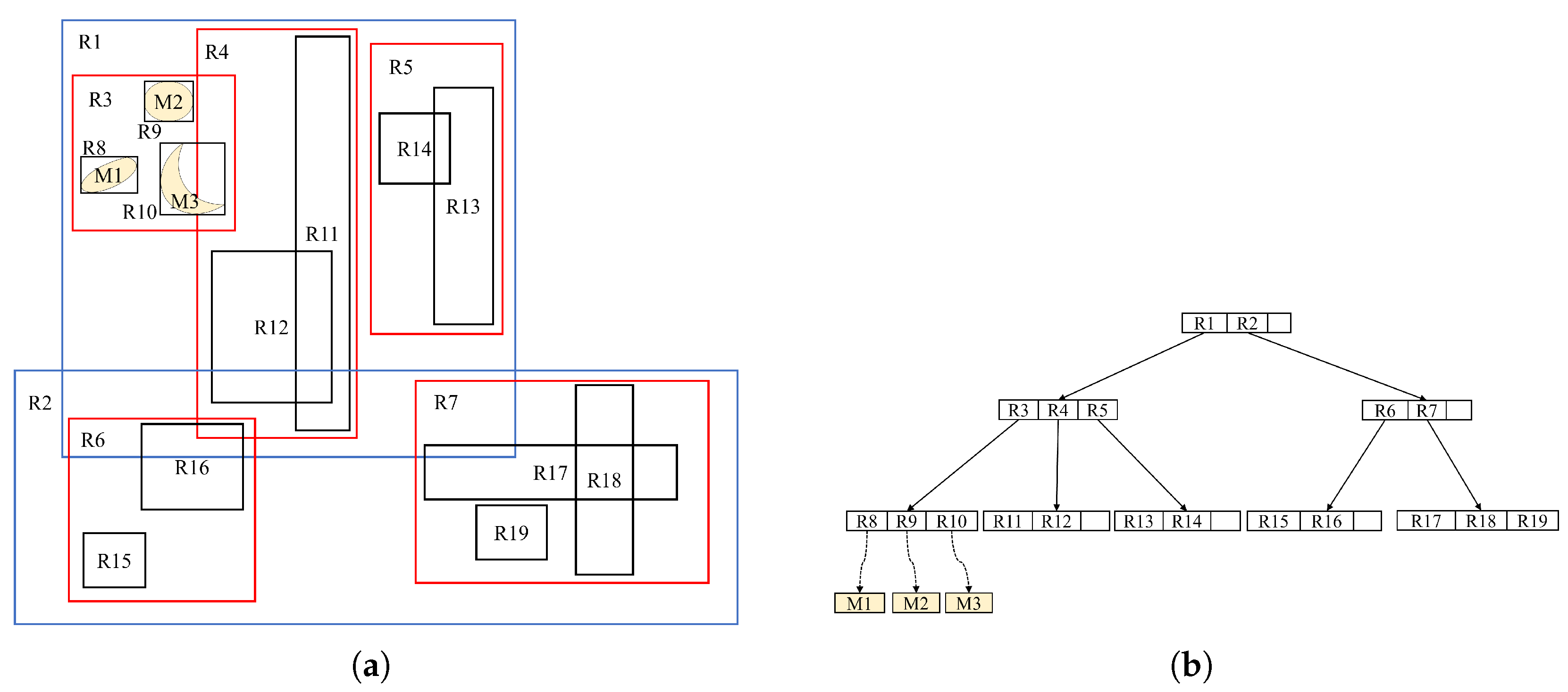
3.2.3. Phenomenon of Cross-Grid Overlap

In R-MLGTI, data is first partitioned into grid cells and then stored using an R-tree structure. Since spatial objects may span multiple grid cells, a non-negligible issue is the phenomenon of cross-grid overlap. Although such occurrences are inevitable in spatial partitioning, we aim to minimize their probability through the appropriate selection of grid levels.
We first conduct a one-dimensional modeling analysis. The problem can be abstracted as a line segment of length L, denoted as the interval [ 0 , L ] , on which there exist n fixed points forming the set P = { x 1 , x 2 , , x n } , where each x i [ 0 , L ] . A sub-segment of length t is randomly selected from the interval, denoted as [ x , x + t ] , where x [ 0 , L t ] to ensure that the sub-segment lies entirely within the original interval. Our objective is to compute the probability that the sub-segment contains at least one point from the set P. Let event A denote that the sub-segment [ x , x + t ] contains at least one point x i . Then,
A = [ x , x + t ] P
To simplify the calculation, we use the complement approach and instead compute the probability of event A c (i.e., the sub-segment contains no points):
P ( A ) = 1 P ( A c )
For each point x i P , in order for it not to be included in the sub-segment, the starting point x must not fall within the interval [ x i t , x i ] . Given that the valid starting range is [ 0 , L t ] , the exclusion interval for each x i can be expressed as
I i = max ( 0 , x i t ) , min ( x i , L t )
This interval represents all possible starting points that would result in x i being included. If the interval is empty (i.e., the bounds do not satisfy the ordering), the point cannot be included in any sub-segment and can be ignored.
For all x i P , we take the union of their corresponding exclusion intervals I i :
U = i = 1 n I i
Let the total length of this union be | U | , representing the range within which selecting a starting point will lead to the sub-segment containing at least one target point. Since the total valid starting range has length L t , the final probability expression becomes
P ( A ) = | U | L t = 1 L t · i = 1 n max ( 0 , x i t ) , min ( x i , L t )
This formula expresses the probability that a randomly selected sub-segment of length t from [ 0 , L ] contains at least one of the target points. Furthermore, this probability can serve as a measure of the likelihood that a spatial object spans multiple grid cells along a single dimension under a given grid level.
For the two-dimensional case, given a dataset D, whose minimum bounding rectangle (MBR) has width t x and height t y (in degrees), and a grid space formed by d-level binary partitioning in both longitude and latitude, the probability P ( D c ) that D does not cross any grid boundary is given by
P ( D c ) = 1 | U | ( L x t x ) ( L y t y ) U = i = 1 2 d max ( 0 , x i t x ) , min ( x i , L x t x ) × max ( 0 , y i t y ) , min ( y i , L y t y )
In the R-MLGTI index structure, we first predict the insertion data using Equation (10). For instance, given a dataset with an MBR size of 30 × 30 , Equation (10) allows us to calculate the probabilities that the data does not cross grids at L e v e l 0 , L e v e l 1 , L e v e l 2 , and  L e v e l 3 as 100 % , 86.96 % , 63.24 % , and  25.30 % , respectively. If the data is inserted at Level2 or earlier in the multi-level dynamic hierarchical grid, the probability of encountering grid-crossing issues is relatively low. For data with a probability less than 60 % of avoiding grid-crossing during insertion, we directly employ a grid-crossing strategy for processing.

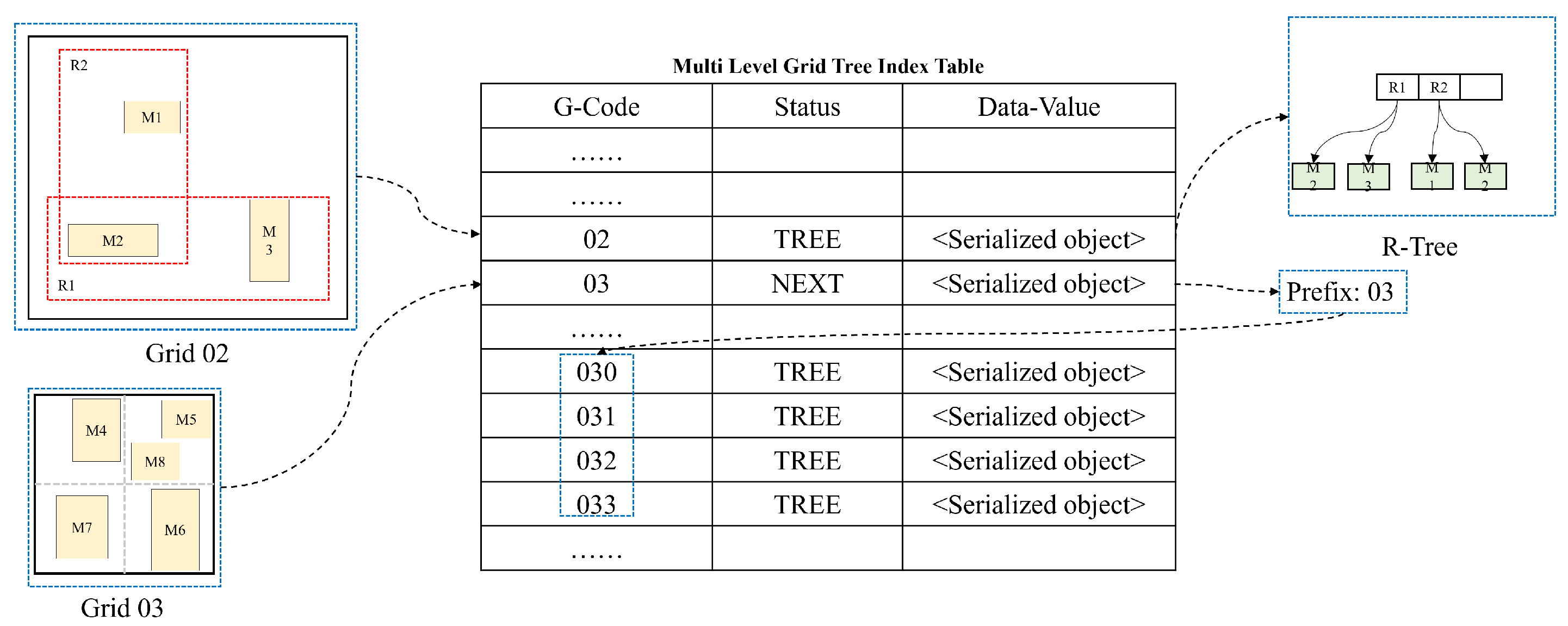
3.2.4. Storage Structure

The storage structure corresponding to the R-MLGTI index model is shown in Figure 5. The grid G ( X i ) is represented by the grid encoding G C o d e , which is derived from the space partitioned by the Z-curve. In persistent storage, based on the concept of inverted indexing, the  G C o d e is used as the primary key, and the S t a t u s field records whether the current grid cell satisfies the condition c ( G ( X i ) ) . When the condition is satisfied, the  S t a t u s field is marked as TREE; otherwise, it is marked as NEXT. The  D a t a V a l u e field stores the address of the corresponding R-tree or the serialized binary object.
Based on the previously mentioned grid-partitioning encoding strategy, when the S t a t u s field is marked as NEXT, it means that the data in the grid cell G ( X i ) will be managed by the next level. The  G C o d e also serves as the prefix for the partition encoding at the next level.

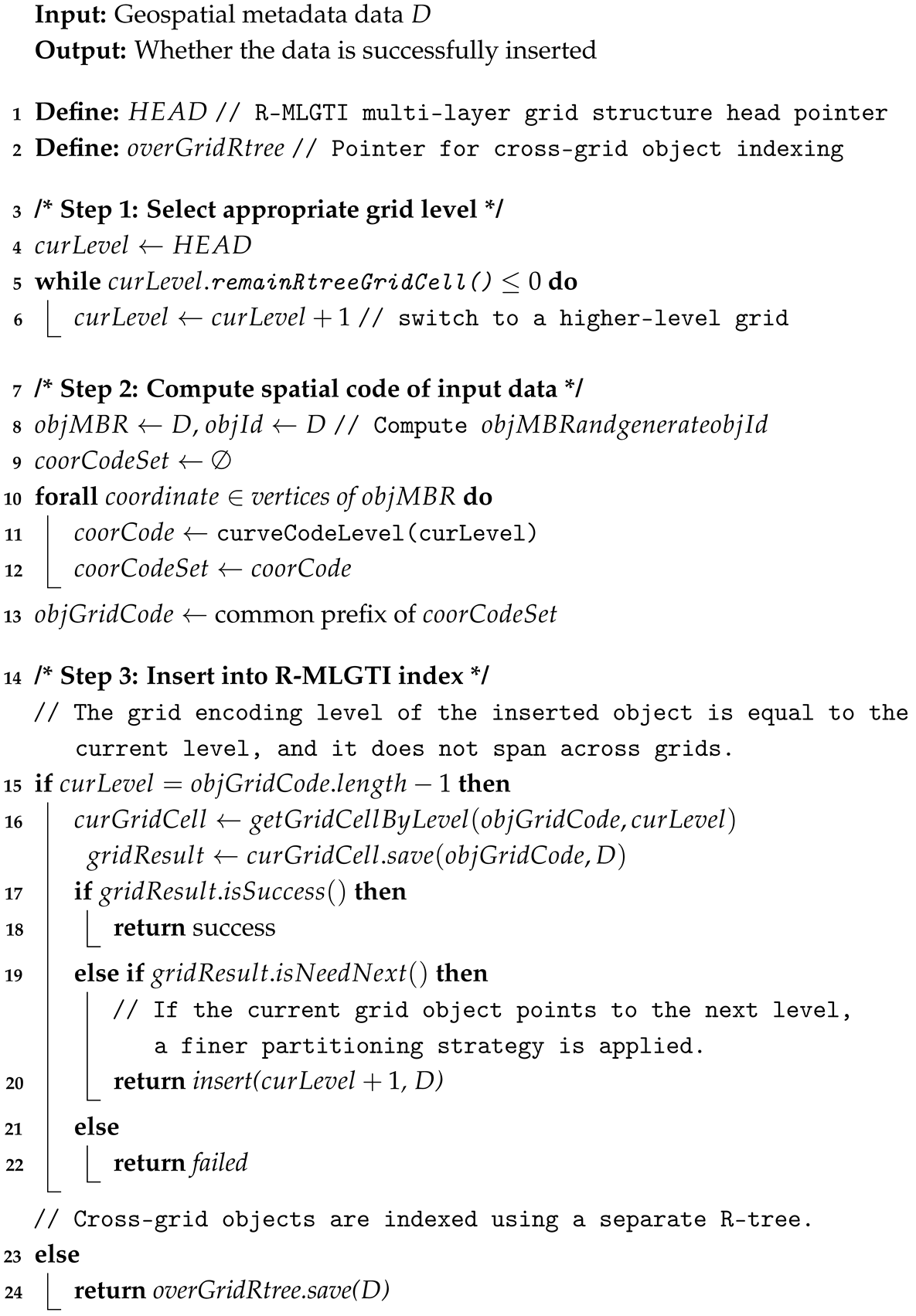
3.3. Insertion Algorithm

Algorithm 1 demonstrates the data insertion steps. Before inserting data, R-MLGTI first initializes the system. The layer-partitioning grid head pointer (HEAD) points to the default partitioning level, and the system cache holds the 1st- and 10th-order Z-curves. When spatial data is inserted, the MBR (minimum bounding rectangle) of the spatial data is calculated as the basic management unit for the geometric information of the subsequent data.
Using the partitioning level specified by HEAD as the reference, the grid encoding corresponding to the four corner points of the MBR is computed. The longest common prefix of these four grid encodings is then taken as the grid encoding for this spatial data. For example, in the case of the second-order partitioning, the four coordinates are 010, 011, 012, and 013. The longest common prefix among these is 01, indicating that the MBR of the spatial data spans across the four grid cells in the 01 region.
For data that spans multiple grid cells, an independent R-tree is used for storage. For MBRs that do not span multiple grids, the grid information corresponding to the current grid encoding is queried, and the S t a t u s and D a t a - V a l u e fields are parsed. If the S t a t u s field is marked as NEXT, it indicates that the grid area does not store information at the current level and that the data will be inserted at the next level. If the S t a t u s field is marked as TREE, it means that the current grid will point to a dedicated R-tree for data storage and the D a t a V a l u e field will point to the corresponding R-tree. The data insertion will then be handled by this R-tree for indexing and storage.
During the insertion process, after the S t a t u s of the grids at the HEAD level is updated to NEXT, HEAD will point to the next level.

3.4. Query Algorithm

In spatial range queries, the R-MLGTI structure naturally isolates each spatial partition, which allows for the full utilization of parallelism to accelerate query efficiency. Algorithm 2 demonstrates the entire query process.
Algorithm 1: Inserting geospatial metadata into R-MLGTI
Ijgi 14 00231 i001
In the retrieval algorithm, two tasks are first started in parallel: one searches within the multi-level grid partition tree, and the other handles cross-grid queries in the independent R-tree. After both tasks are completed, their result sets are merged to complete the spatial query. Based on the ID information in the result sets, the complete data information is then queried. The retrieval process within the multi-level grid partition tree is described in detail by Algorithm 3.
In Algorithm 3, the first step is to calculate the portions of grids that intersect the query region’s MBR. These intersecting grids are then divided into two categories: the first category consists of grids that are fully enclosed within the query region, and the second category consists of grids that are partially located within the query region’s MBR.
Algorithm 2: Spatial data query
Ijgi 14 00231 i002
Algorithm 3: Query in multi-level grid tree
Ijgi 14 00231 i003
For the first category, all data within the grid can be directly returned. For the second category, the R-tree pointed to by the grid must be retrieved, and a query is performed on the R-tree.
Regardless of the category, processing is performed in parallel at the grid level, which significantly improves retrieval efficiency compared to serial execution.

4. Experiments and Results

4.1. Environment and Testing Methodology

4.1.1. Platform and Environment

The experimental operating system was Microsoft Windows 10 (64-bit)(Microsoft Corporation, Redmond, WA, USA). The development environment used IntelliJ IDEA Community Edition 2024, with Java as the programming language. The hardware environment was configured as follows: Intel(R) Core(TM) i5-12400F CPU @ 2.50 GHz, 12 cores, and 32 GB of RAM.

4.1.2. Test Method

To evaluate the effectiveness of R-MLGTI in handling large-scale and unevenly distributed spatial data, we implemented the memory prototype system of the R-MLGTI index structure using Java(OpenJDK 11.0.2). The comparative models included the R-tree [45] implemented by Dave Moten, the Hilbert-R-tree [46] implemented by “TheDeathFar”, and the grid-indexing method based on the Z-curve.
The R-MLGTI proposed in this paper involves hyperparameters such as the grid division level, the selection of trees within the tree structure, and the number of subtrees per tree. Table 1 lists the various model variants and their parameter settings used in the experiments. In the subsequent experiments, we evaluated multiple R-MLGTI variants based on the parameter settings listed in the table.
The benchmark test was conducted using the Java Microbenchmark Harness (JMH) tool [47]. Before the actual measurement, five warm-up iterations were carried out, each lasting 10 s. The purpose of the preheating phase was to ensure that performance measurements were conducted after the Java Virtual Machine (JVM) reached a stable state, thereby minimizing the impact of transient startup behavior and ensuring that the results were representative and consistent. This paper adopts the average execution time as the main performance evaluation index (11). Specifically, after the preheating stage was completed, each test method was independently executed n times; the time-consuming results of each execution were recorded, and their arithmetic mean was taken. During both the data import and query processes, n was set to 10.
T ¯ = 1 n i = 1 n T i

4.1.3. Code Warm-Up

Java applications run on the JVM, which employs a variety of dynamic optimizations during runtime. Initially, when code is executed for the first time, the JVM typically interprets bytecode, resulting in relatively low execution performance. As the execution continues, the JVM identifies frequently used methods—so-called “hot” methods—and compiles them into native machine code through Just-In-Time (JIT) compilation. In addition to JIT, the JVM performs other runtime optimizations such as method inlining, loop unrolling, escape analysis, and lock elimination. These optimizations are not applied immediately but are instead triggered after the code has been executed multiple times and meets specific heuristics defined by the JVM.
If performance measurements are taken without sufficient warm-up, the results will likely reflect early-stage JVM behavior, including interpretation overhead, class-loading delays, and memory-allocation irregularities. Such measurements are misleading, as they do not capture the actual performance characteristics of code under typical long-running conditions. To address this, JMH incorporates a warm-up mechanism that repeatedly invokes benchmark methods before actual measurement begins. This warm-up process gives the JVM adequate time to compile and optimize the relevant code paths, ensuring that performance measurements are taken under optimized and stable conditions.
In this experiment, each warm-up iteration lasted 10 s, and a total of five iterations were conducted before the actual benchmarking phase. During the formal testing stage, each method was executed ten times, and the average execution time was recorded as the final performance metric. This approach balances JVM optimization stability with practical benchmarking efficiency and helps eliminate performance fluctuations caused by JVM startup behavior, thereby producing results that more closely reflect real-world application performance.

4.2. Experimental Data

The smallest unit indexed by R-MLGTI is the minimum bounding rectangle (MBR) of geospatial data. To evaluate the performance of R-MLGTI, we first generated simulated datasets of varying scales, including 10,000, 100,000, and 1,000,000 entries, with uneven spatial distributions. These datasets were divided into dense and sparse regions, with a distribution ratio of 0.91:0.03. Specifically, when creating the artificial data, we proceeded as described below.
First, to ensure that the datasets we created had uneven distributions, we partitioned the entire index space. We divided the global area into four regions based on the 0° longitude and 0° latitude, which we refer to as the top-left, top-right, bottom-left, and bottom-right regions.
In these four regions, we defined the weight for the number of data entries to be created in each region to achieve the goal of generating non-uniformly distributed data: the top-left region had a weight of 0.91, and the top-right, bottom-left, and bottom-right regions each had a weight of 0.03. The sum of the weights for the four regions totaled 1. For example, with the above weight distribution, when we specify the total number of artificial data entries to be 1000, the expected number of data entries for the top-left region will be 910, while the expected number for each of the remaining three regions will be 3. By setting these weights, we create an overall non-uniform distribution for the artificial datasets.
Next, we generated data for each region based on the desired total number of entries and the weight proportion of each region. More specifically, we generated the bounding rectangle for the data. Taking the data generation process for the top-left region as an example, the method for generating the bounding rectangle for each data entry was as follows: (1) Determine the region boundary: The longitude range of the top-left region was from −180° to 0°, and the latitude range was from 0° to 90°. (2) Randomly generate two longitude offsets and two latitude offsets within the region boundaries. These four randomly generated variables, combined with the region boundaries, form a rectangle within the top-left region.
Finally, to visually represent these data (the distribution of bounding rectangles), we calculated the geometric center of each bounding rectangle and used these centers to plot the artificial datasets across the global spatial range. Figure 6a shows the distribution of the dataset containing 10,000 entries.
To further assess the performance of R-MLGTI on real-world spatial datasets, we downloaded Landsat 7 satellite data released by the United States Geological Survey (USGS). This dataset spans from 1999 to 2018 and contains a total of 2,585,203 geospatial records [48]. Its spatial distribution is shown in Figure 6b, where land areas are significantly denser compared to oceanic regions.

4.3. Results and Analysis

4.3.1. Performance of Data Import

The performance of different indexing methods for data import on the simulated datasets and the Landsat 7 dataset is shown in Figure 7. The R-tree method demonstrated the best performance during the data import process and its time consumption grew relatively slowly as the data scale increased, indicating good scalability. In contrast, both the R-MLGTI and the grid-indexing methods exhibited significant increases in time consumption as the data scale grew, reflecting poor scalability.
The time consumption of the R-tree structure mainly stems from the comparison of the MBRs of the intermediate nodes during the data insertion process, as it traverses from the root node down. Although node splits may occur to maintain overall balance, the data insertion algorithm remains relatively simple. On the other hand, the grid-indexing method requires the calculation of spatial encoding for the inserted spatial objects, which is a more time-consuming process. Since R-MLGTI combines the two indexing methods mentioned above, it exhibits the worst performance in the data import and indexing process. Additionally, R-MLGTI does not fully leverage the parallelism advantages provided by grid partitioning during the data insertion process, which still need to be optimized in future work. However, this paper focuses on the spatial query performance of R-MLGTI, as fast querying is one of the fundamental purposes of indexing spatial data.

4.3.2. Performance of Spatial Query

In the experiments on the simulated dataset, regions A, B, and C, as shown in Figure 8, were selected for query benchmarking. Each of the selected test regions A, B, and C corresponds to an MBR of 40° × 40° in size, with distinct characteristics. Region A has a relatively uniform and dense data distribution, region B has a relatively uniform but sparse data distribution, and region C has an uneven data distribution. Although the distribution of these three regions can only be determined after knowing the data locations, during the incremental insertion of data, these regions encompass all possible query areas at a certain retrieval moment.
The performance of R-MLGTI on various simulated datasets is shown in Figure 9. At first, R-MLGTI’s query efficiency was worse than that of the other methods on small-scale simulated datasets, but as the data size grew, its performance gradually surpassed that of the other two methods. Taking 1,000,000 simulated data points as an example, the average performance of each method across three query regions (A, B, and C) was as follows: R-MLGTI took an average of 6409.66 microseconds, which was 56.80% faster than the R-tree method and 14.85% faster than the grid-indexing method.
We can draw the following conclusions:
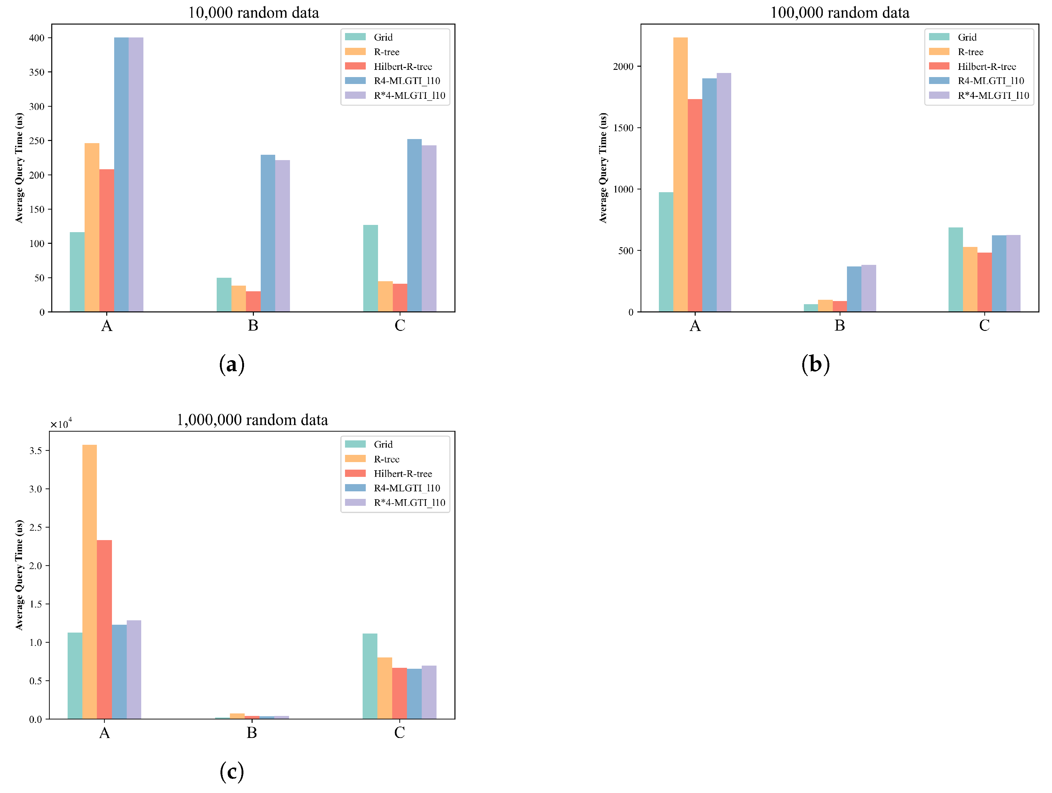
  • As the data scale increases, the retrieval time for all methods increases across the various query regions.
  • The R-tree index is more advantageous for unevenly distributed data or smaller datasets. The experiment confirms the conclusion that excessive overlap of intermediate-node MBRs in the R-tree due to large data volumes negatively affects query efficiency. Therefore, it is best to avoid using a single R-tree index when the indexed objects are overly concentrated.
  • The advantage of the grid index lies in its ability to maintain good performance when handling large amounts of uniformly distributed data. This is due to the fixed-partition structure of the grid, which divides the global latitude and longitude ranges and encodes the grid cells. Spatial information can then be queried using only the grid encoding field. However, the indexing performance deteriorates when the grid cells are of fixed size and the data is unevenly distributed.
  • R-MLGTI, which combines the grid-partitioning concept and uses independent R-tree indexing for each partition, has a more complex structure. It actually incurs more query time when the data scale is small. As the data scale increases, the query performance gap between R-MLGTI and the other two methods gradually narrows, with a smaller increase in query time. It is more suitable for querying large-scale, unevenly distributed data.
On the Landsat 7 dataset, we selected different query window sizes: 40° × 40°, 20° × 20°, and 10° × 10°. As mentioned in Section 4.2, the data over the land is more concentrated, while the data over the ocean is sparser. Therefore, we defined three different regions, A, B, and C, on the same query window size, located in the land area, the ocean area, and the land–ocean boundary area, respectively. As shown in Figure 10, “A-40” represents a 40° × 40° window size located in the land area with dense data distribution.
The performance of each method is shown in Figure 11. Grouped by query window size, for the 40 × 40 query window, R-MLGTI was 19.11% faster than the R-tree method and 54.60% faster than the grid-indexing method. For the 20 × 20 query window, R-MLGTI was 14.57% faster than the R-tree method and 75.43% faster than the grid-indexing method. For the 10 × 10 query window, R-MLGTI was 2.92% slower than the R-tree method but 53.81% faster than the grid-indexing method. It can be seen that R-MLGTI also demonstrated superior overall performance on real datasets:
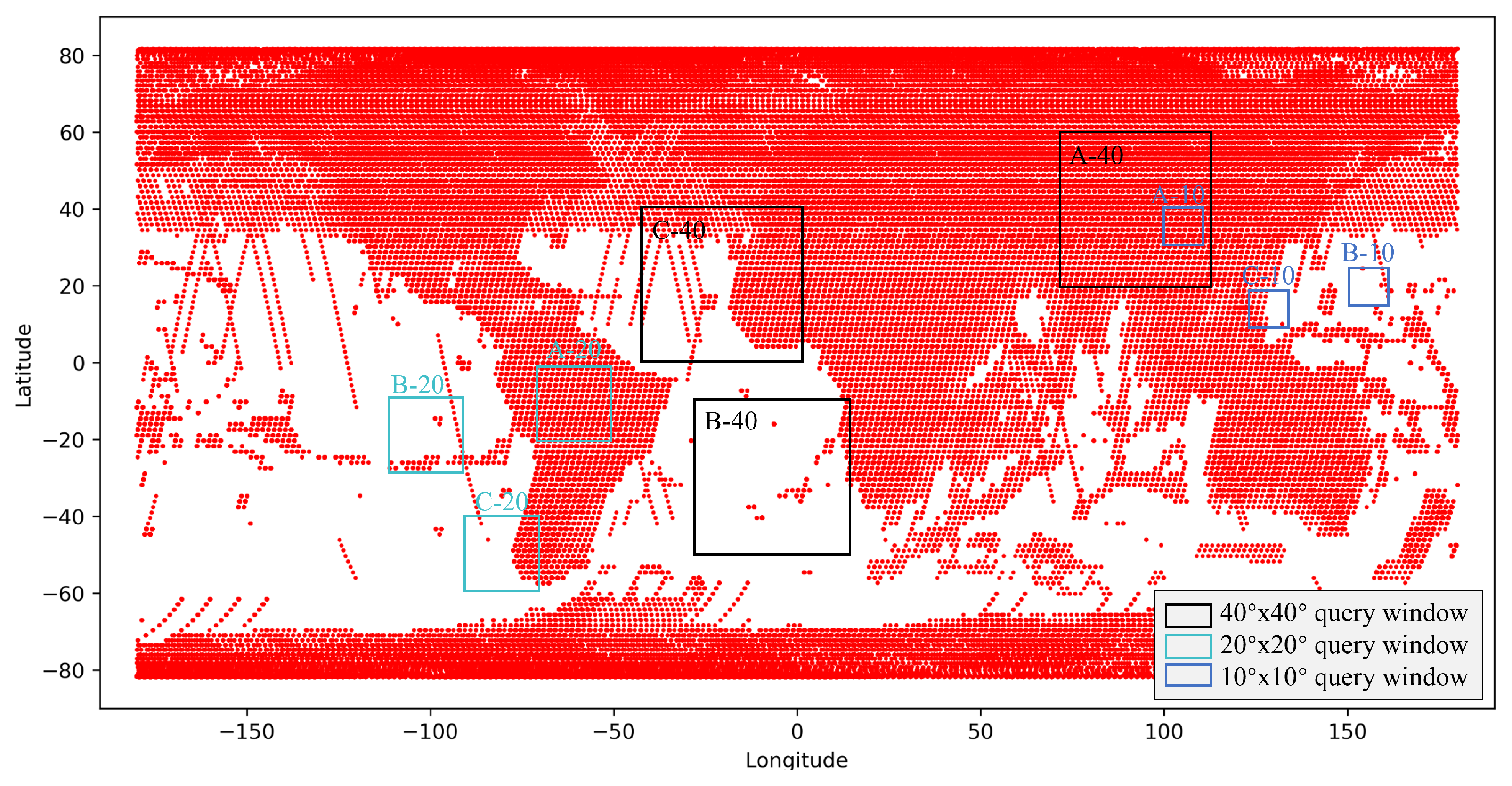
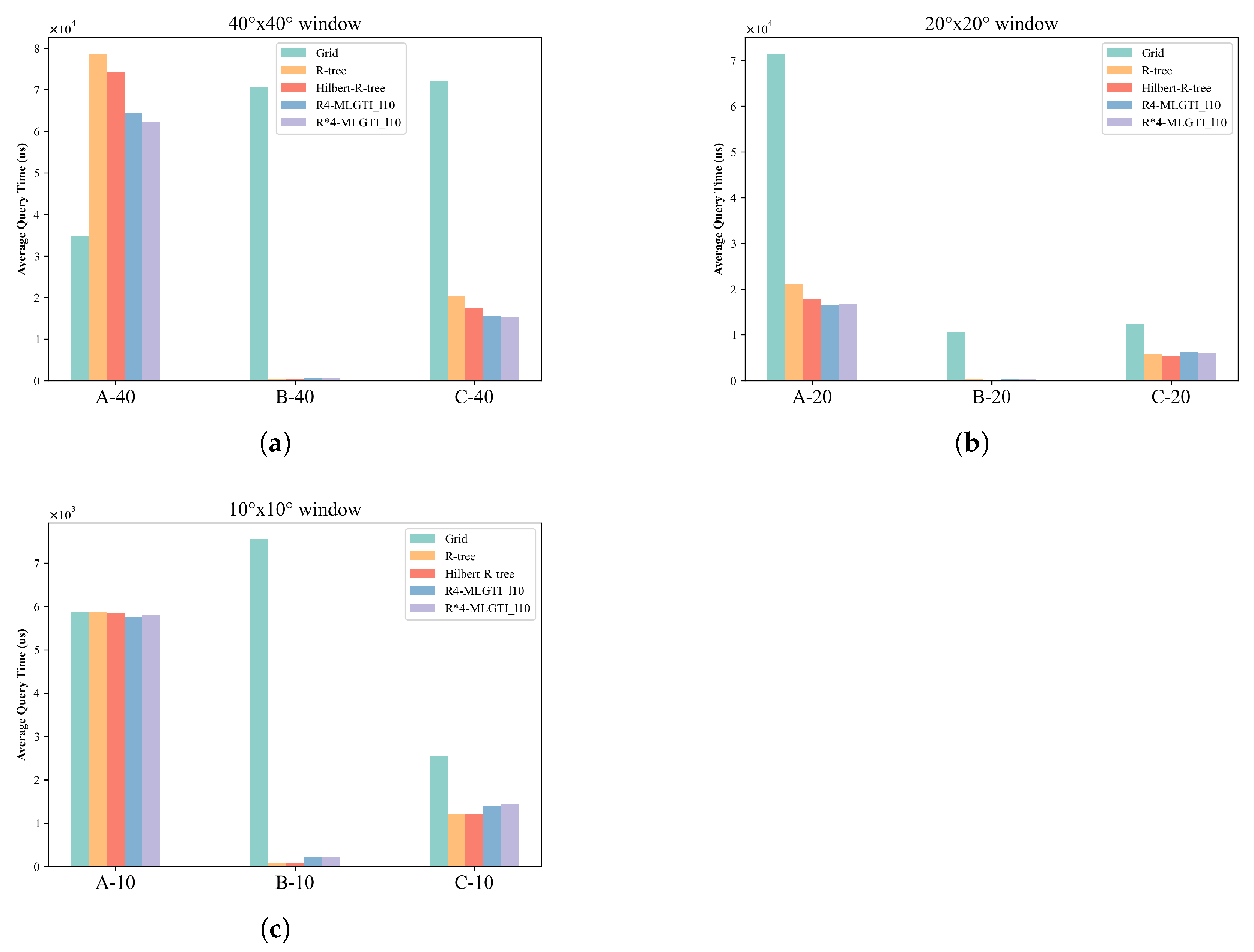
  • The grid-indexing method only had an advantage when the query window was sufficiently large and contained a large amount of data; otherwise, its performance was worse than that of the R-tree and R-MLGTI methods.
  • The advantage of the R-tree method was similar on the simulated data. In datasets with uneven distribution and the same query window size, the R-tree method performed better when the data distribution was sparse (i.e., fewer data points per unit area).
  • The R-MLGTI method performed better in large-scale data retrieval or regions with non-uniform distribution, and it outperformed the R-tree method on dense data retrieval over large areas.
Overall, the R-tree method is well-suited for handling small-scale datasets with uneven distribution, particularly excelling in scenarios with sparse data distribution. However, as the data scale increases or the data becomes overly concentrated, the overlapping of MBRs in intermediate nodes significantly reduces performance. The grid-indexing method is ideal for large-scale datasets with a uniform distribution, benefiting from its fixed-partition structure and efficient querying mechanism based on grid encoding. However, it struggles with indexing failures when dealing with unevenly distributed data. R-MLGTI combines the advantages of grid partitioning and independent R-tree indexing within partitions, making it well-suited for large-scale queries, especially for unevenly distributed data. It outperforms the R-tree in querying densely populated regions, but due to its complexity, its performance is slightly inferior to that of other methods when the data scale is small.

5. Discussion

The R-MLGTI indexing model demonstrates clear advantages in addressing the challenges of spatial range queries on large-scale and unevenly distributed spatial datasets. By integrating grid partitioning with R-tree indexing and leveraging the parallelism potential of grid structures, R-MLGTI achieves a balanced trade-off between indexing flexibility and query efficiency. Experimental results on both synthetic and real-world datasets further validate the model’s capability to maintain low query latency under such complex spatial distributions. Despite these strengths, R-MLGTI also presents several limitations.
First, the current in-memory implementation does not fully exploit the potential for parallelism during the data import phase. In particular, the computation of the cost function c ( G ) and the management of the hybrid grid–R-tree structure introduce significant overhead. Maintaining index stability during dynamic data changes also requires considerable processing time. These factors collectively hinder the performance of R-MLGTI in terms of data ingestion efficiency.
Second, the applicability of R-MLGTI is scenario-dependent. Its strengths are most evident when indexing large-scale, highly skewed spatial datasets. However, in more uniformly distributed or smaller-scale scenarios, the indexing performance does not provide clear benefits, and it may even underperform compared to simpler indexing structures. In addition, we used the above experimental data to conduct more complex queries, such as nearest-neighbor queries, using R-MLGTI, but its performance did not show an advantage compared with traditional methods. This limits the general applicability of the model in broader spatial data management tasks.

6. Conclusions

This paper presents the R-MLGTI data-indexing method, designed for efficient range queries on large-scale spatial data with an uneven distribution. R-MLGTI combines the advantages of grid partitioning and independent R-tree indexing within each partition. This hybrid structure offers flexibility in indexing and achieves improved query performance, particularly when handling large-scale, non-uniformly distributed spatial data and high-density regions. Experiments based on real datasets validate the query capabilities of R-MLGTI and demonstrate that integrating grid partitioning with R-tree indexing yields better performance compared to using a single indexing method alone, especially in scenarios involving uneven spatial data distributions.
Although the in-memory implementation of R-MLGTI offers advantages in querying, the data import process cannot fully utilize the grid partition structure to achieve parallel operations. Additionally, the complex structure of the R-MLGTI index lacks a persistence solution based on a database. Future directions include integration with databases such as PostgreSQL and HBase for persistent data storage.

Author Contributions

All authors contributed to this study’s conception and design. Yuqin Li wrote the manuscript and conceptualized the experiments. Jining Yan proposed the algorithm idea and guided the manuscript writing. Xiaohui Huang provided the experimental data and guidance on the algorithmic processes. Xiangyou He conducted supplementary experiments and summarized the results. Ze Deng validated the findings. Yunliang Chen reviewed and edited the manuscript. All authors have read and agreed to the final version of the manuscript.

Funding

This work was supported in part by the National Natural Science Foundation of China under Grant 42471505, in part by Guangxi Key Researchand Development Program under Grant Guike AB25069111, and in part by the National Key Research and Development Program of China under Grant2022 YFC3800700.

Institutional Review Board Statement

Not applicable.

Informed Consent Statement

Not applicable.

Data Availability Statement

The Landsat 7 Enhanced Thematic Mapper Plus Level-1, Collection 1 data (2017) used in this study are publicly available from the U.S. Geological Survey’s Earth Resources Observation and Science (EROS) Center at https://doi.org/10.5066/F7WH2P8G/ (accessed on 12 January 2025).

Conflicts of Interest

The authors declare no conflicts of interest.

References

  1. Chen, J.; Wang, L.; Zhao, X.; Cheng, S. The relationship between urbanization and land use in Guiyang city. Earth Sci. 2019, 44, 2944–2954. [Google Scholar]
  2. Xiao, Y.; Wang, Q.; Zhang, H.K. Global Natural and Planted Forests Mapping at Fine Spatial Resolution of 30 m. J. Remote Sens. 2024, 4, 0204. [Google Scholar] [CrossRef]
  3. Sheng, M.; Lei, L.; Zeng, Z.C.; Rao, W.; Song, H.; Wu, C. Global land 1° mapping dataset of XCO2 from satellite observations of GOSAT and OCO-2 from 2009 to 2020. Big Earth Data 2023, 7, 170–190. [Google Scholar] [CrossRef]
  4. Li, M.; Peng, J.; Lu, Z.; Zhu, P. Research progress on carbon sources and sinks of farmland ecosystems. Resour. Environ. Sustain. 2023, 11, 100099. [Google Scholar] [CrossRef]
  5. Tian, J.; Zhang, Y.; Zhang, X. Impacts of heterogeneous CO2 on water and carbon fluxes across the global land surface. Int. J. Digit. Earth 2021, 14, 1175–1193. [Google Scholar] [CrossRef]
  6. Shekhar, S.; Evans, M.R.; Gunturi, V.; Yang, K.; Cugler, D.C. Benchmarking spatial big data. In Proceedings of the Specifying Big Data Benchmarks: First Workshop, WBDB 2012, San Jose, CA, USA, 8–9 May 2012, and Second Workshop, WBDB 2012, Pune, India, 17–18 December 2012; Revised Selected Papers. Springer: Berlin/Heidelberg, Germany, 2014; pp. 81–93. [Google Scholar]
  7. Tong, X.; Ben, J.; Liu, Y.; Zhang, Y. Modeling and expression of vector data in the hexagonal discrete global grid system. Int. Arch. Photogramm. Remote Sens. Spat. Inf. Sci. 2013, 40, 15–25. [Google Scholar] [CrossRef]
  8. Li, S.; Pu, G.; Cheng, C.; Chen, B. Method for managing and querying geo-spatial data using a grid-code-array spatial index. Earth Sci. Inform. 2019, 12, 173–181. [Google Scholar] [CrossRef]
  9. Jagadish, H.V.; Ooi, B.C.; Tan, K.L.; Yu, C.; Zhang, R. iDistance: An adaptive B+-tree based indexing method for nearest neighbor search. ACM Trans. Database Syst. (TODS) 2005, 30, 364–397. [Google Scholar] [CrossRef]
  10. Guttman, A. R-trees: A dynamic index structure for spatial searching. In Proceedings of the 1984 ACM SIGMOD International Conference on Management of Data, Boston, MA, USA, 18–21 June 1984; pp. 47–57. [Google Scholar]
  11. Li, G.; Tang, J. A new R-tree spatial index based on space grid coordinate division. In Proceedings of the 2011, International Conference on Informatics, Cybernetics, and Computer Engineering (ICCE2011), Melbourne, Australia, 19–20 November 2011; Volume 2: Information Systems and Computer Engineering. Springer: Berlin/Heidelberg, Germany, 2012; pp. 133–140. [Google Scholar]
  12. Sellis, T.; Roussopoulos, N.; Faloutsos, C. The R+-tree: A dynamic index for multi-dimensional objects. In Proceedings of the 13th VLDB Conference, Brighton, UK, 1–4 September 1987. [Google Scholar]
  13. Kamel, I.; Faloutsos, C. Hilbert R-Tree: An Improved Rtree Using Fractals. In Proceedings of the VLDB, Citeseer, Santiago de Chile, Chile, 12–15 September 1994; Volume 94, pp. 500–509. [Google Scholar]
  14. Amiri, A.M.; Samavati, F.; Peterson, P. Categorization and conversions for indexing methods of discrete global grid systems. ISPRS Int. J. Geo-Inf. 2015, 4, 320–336. [Google Scholar] [CrossRef]
  15. Zhou, M.; Chen, J.; Gong, J. A pole-oriented discrete global grid system: Quaternary quadrangle mesh. Comput. Geosci. 2013, 61, 133–143. [Google Scholar] [CrossRef]
  16. Huang, M.; Hu, P.; Xia, L. A grid based trajectory indexing method for moving objects on fixed network. In Proceedings of the 2010 18th International Conference on Geoinformatics, Beijing, China, 18–20 June 2010; pp. 1–4. [Google Scholar]
  17. Nievergelt, J.; Hinterberger, H.; Sevcik, K.C. The grid file: An adaptable, symmetric multikey file structure. ACM Trans. Database Syst. (TODS) 1984, 9, 38–71. [Google Scholar] [CrossRef]
  18. Ficklin, D.L.; Letsinger, S.L.; Gholizadeh, H.; Maxwell, J.T. Incorporation of the Penman–Monteith potential evapotranspiration method into a Palmer Drought Severity Index tool. Comput. Geosci. 2015, 85, 136–141. [Google Scholar] [CrossRef]
  19. Guan, X.; Bo, C.; Li, Z.; Yu, Y. ST-hash: An efficient spatiotemporal index for massive trajectory data in a NoSQL database. In Proceedings of the 2017 25th International Conference on Geoinformatics, Buffalo, NY, USA, 2–4 August 2017; pp. 1–7. [Google Scholar]
  20. Huang, Z. Research on Hybrid Index Based on Multi-Level Grid and STR Tree. Master’s Thesis, Zhejiang University, Hangzhou, China, 2013. [Google Scholar]
  21. Tang, X.; Han, B.; Chen, H. A hybrid index for multi-dimensional query in HBase. In Proceedings of the 2016 4th International Conference on Cloud Computing and Intelligence Systems (CCIS), Beijing, China, 17–19 August 2016; pp. 332–336. [Google Scholar]
  22. Sieranoja, S. High Dimensional kNN-Graph Construction Using Space Filling Curves. Master’s Thesis, Itä-Suomen yliopisto, Joensuu, Finland, 2015. [Google Scholar]
  23. Laurini, R.; Thompson, D. Fundamentals of Spatial Information Systems; Academic Press: Cambridge, MA, USA, 1992; Volume 37. [Google Scholar]
  24. Zhai, W.; Qi, C.; Cheng, C.; Li, S. Spatial data management method with GeoSOT grid. In Proceedings of the 2017 IEEE International Geoscience and Remote Sensing Symposium (IGARSS), Fort Worth, TX, USA, 23–28 July 2017; pp. 5217–5220. [Google Scholar]
  25. Cheng, C.; Tong, X.; Chen, B.; Zhai, W. A subdivision method to unify the existing latitude and longitude grids. ISPRS Int. J. Geo-Inf. 2016, 5, 161. [Google Scholar] [CrossRef]
  26. Qi, K.; Cheng, C.; Hu, Y.; Fang, H.; Ji, Y.; Chen, B. An improved identification code for city components based on discrete global grid system. ISPRS Int. J. Geo-Inf. 2017, 6, 381. [Google Scholar] [CrossRef]
  27. Li, S.; Cheng, C.; Chen, B.; Meng, L. Integration and management of massive remote-sensing data based on GeoSOT subdivision model. J. Appl. Remote Sens. 2016, 10, 34003. [Google Scholar] [CrossRef]
  28. Zhai, W.; Yang, Z.; Wang, L.; Wu, F.; Cheng, C. The non-sql spatial data management model in big data time. In Proceedings of the 2015 IEEE international geoscience and remote sensing symposium (IGARSS), Milan, Italy, 26–31 July 2015; pp. 4506–4509. [Google Scholar]
  29. Tong, X.; Wang, R.; Wang, L.; Lai, G.; Ding, L. An efficient integer coding and computing method for multiscale time segment. Acta Geod. Cartogr. Sin. 2016, 45, 66. [Google Scholar]
  30. Qu, T.; Wang, L.; Yu, J.; Yan, J.; Xu, G.; Li, M.; Cheng, C.; Hou, K.; Chen, B. STGI: A spatio-temporal grid index model for marine big data. Big Earth Data 2020, 4, 435–450. [Google Scholar] [CrossRef]
  31. Liu, H.; Yan, J.; Huang, X. HBase-based spatial-temporal index model for trajectory data. In IOP Conference Series: Earth and Environmental Science; IOP Publishing: Bristol, UK, 2022; Volume 1004, p. 12007. [Google Scholar]
  32. Guo, N.; Xiong, W.; Wu, Y.; Chen, L.; Jing, N. A geographic meshing and coding method based on adaptive Hilbert-Geohash. IEEE Access 2019, 7, 39815–39825. [Google Scholar] [CrossRef]
  33. Huang, X.; Deng, Z.; Yan, J.; Li, J.; Chen, Y.; Wang, L. A high-performance spatial range query-based data discovery method on massive remote sensing data via adaptive geographic meshing and coding. IEEE J. Miniaturization Air Space Syst. 2020, 2, 117–128. [Google Scholar] [CrossRef]
  34. Wu, Y.; Cao, X.; An, Z. A spatiotemporal trajectory data index based on the Hilbert curve code. In IOP Conference Series: Earth and Environmental Science; IOP Publishing: Bristol, UK, 2020; Volume 502, p. 12005. [Google Scholar]
  35. Wang, X.; Sun, Y.; Sun, Q.; Lin, W.; Wang, J.Z.; Li, W. HCIndex: A Hilbert-Curve-based clustering index for efficient multi-dimensional queries for cloud storage systems. Clust. Comput. 2023, 26, 2011–2025. [Google Scholar] [CrossRef]
  36. Yang, J.; Huang, X. A hybrid spatial index for massive point cloud data management and visualization. Trans. GIS 2014, 18, 97–108. [Google Scholar] [CrossRef]
  37. Gong, J.; Zhu, Q.; Zhang, Y.; Li, X.; Zhou, D. A sub-three-dimensional R-tree index expansion method that takes into account multiple levels of detail. J. Surv. Mapping 2011, 40, 249–255. [Google Scholar]
  38. Sharifzadeh, M.; Shahabi, C. Vor-tree: R-trees with Voronoi diagrams for efficient processing of spatial nearest neighbor queries. Proc. VLDB Endow. 2010, 3, 1231–1242. [Google Scholar] [CrossRef]
  39. Gong, J.; Ke, S.; Zhu, Q.; Zhong, R. A LiDAR point cloud data management method integrating octree and 3D R-tree. J. Surv. Mapping 2012, 41, 597–604. [Google Scholar]
  40. Song, X.; Liu, X.; Zhang, Z.; Wang, D.; Li, C. Research on the spatial index structure of hybrid tree in 3D GIS. J. Shenyang Jianzhu Univ. 2006, 22, 377–381. [Google Scholar]
  41. Liu, Y.; Hao, T.; Gong, X.; Kong, D.; Wang, J. Research on hybrid index based on 3D multi-level adaptive grid and R+ Tree. IEEE Access 2021, 9, 146010–146022. [Google Scholar] [CrossRef]
  42. Liu, Z.; Chen, L.; Yang, A.; Ma, M.; Cao, J. Hiindex: An efficient spatial index for rapid visualization of large-scale geographic vector data. ISPRS Int. J. Geo-Inf. 2021, 10, 647. [Google Scholar] [CrossRef]
  43. Zhang, Y.; Zhang, A.; Gao, M.; Liang, Y. Research on Three-Dimensional Electronic Navigation Chart Hybrid Spatial Index Structure Based on Quadtree and R-Tree. ISPRS Int. J. Geo-Inf. 2022, 11, 319. [Google Scholar] [CrossRef]
  44. Gao, J.; Cao, X.; Yao, X.; Zhang, G.; Wang, W. LMSFC: A Novel Multidimensional Index Based on Learned Monotonic Space Filling Curves. Proc. VLDB Endow. 2023, 16, 2605–2617. [Google Scholar] [CrossRef]
  45. R-Tree Implementation in Java. Available online: https://github.com/davidmoten/rtree (accessed on 12 January 2025).
  46. TheDeathFar. An Implementation of HilbertTree by Java. 2022. Available online: https://github.com/TheDeathFar/HilbertTree (accessed on 12 January 2025).
  47. Java Microbenchmark Harness (JMH). Available online: https://openjdk.org/projects/code-tools/jmh/ (accessed on 12 January 2025).
  48. Landsat 7 Enhanced Thematic Mapper Plus Level-1, Collection 1 [Dataset]. 2017. Available online: https://www.usgs.gov/centers/eros/science/usgs-eros-archive-landsat-archives-landsat-7-enhanced-thematic-mapper-plus-etm?qt-science_center_objects=0#qt-science_center_objects (accessed on 12 January 2025).
Figure 1. R-tree structure: (a) Division of MBRs of spatial objects. (b) Structure of the tree.
Ijgi 14 00231 g001
Figure 2. Static grid partitioning: (a) Spatial data spans multiple grids. (b) Query region spans multiple grids.
Ijgi 14 00231 g002
Figure 3. Structure of R-MLGTI.
Ijgi 14 00231 g003
Figure 4. Data indexing example.
Ijgi 14 00231 g004
Figure 5. Storage structure of the multi-level grid and R-tree hybrid index model.
Ijgi 14 00231 g005
Figure 6. Distribution of simulated data and Landsat 7 ETM (1999–2018): (a) Distribution of 10,000 simulated data records. (b) Distribution of Landsat 7 ETM (1999–2018).
Ijgi 14 00231 g006
Figure 7. Data import benchmarks.
Ijgi 14 00231 g007
Figure 8. Query windows on simulated data.
Ijgi 14 00231 g008
Figure 9. Query results on simulated data: (a) 10,000 random-data query results. (b) 100,000 random-data query results. (c) 1,000,000 random-data query results.
Ijgi 14 00231 g009
Figure 10. Query window sizes and regions on the Landsat 7 dataset.
Ijgi 14 00231 g010
Figure 11. Comparison of retrieval efficiency across different query regions on the Landsat 7 dataset: (a) 40°×40° window. (b) 20°×20° window. (c) 10°×10° window.
Ijgi 14 00231 g011
Table 1. R-MLGTI variants and parameter settings.
No.R-MLGTI VariantMax. Grid LevelMax. Level Grid Resolution 1Child Num. of TreesTree Type
1 R 4 M L G T I l 8 8 1.4063 × 0.7031 4R
2 R 4 M L G T I l 10 10 0.3516 × 0.1758 4R
3 R 4 M L G T I l 15 15 0.0110 × 0.0055 4R
4 R * 4 M L G T I l 10 10 0.3516 × 0.1758 4R*
5 R 6 M L G T I l 10 10 0.3516 × 0.1758 6R
1 The grid resolution column denotes the spatial resolution (longitude × latitude) of the grid at the corresponding partition level, representing the size of each individual grid cell. For example, at level 15, the grid resolution is approximately 1.221 km × 0.611 km, which is sufficient to meet the requirements of most geospatial data indexing scenarios.
Disclaimer/Publisher’s Note: The statements, opinions and data contained in all publications are solely those of the individual author(s) and contributor(s) and not of MDPI and/or the editor(s). MDPI and/or the editor(s) disclaim responsibility for any injury to people or property resulting from any ideas, methods, instructions or products referred to in the content.

