A Fourier Fitting Method for Floating Vehicle Trajectory Lines

Abstract

With the advancement of spatial positioning technology, trajectory data have been growing rapidly. Trajectory data record the spatiotemporal information and behavioral characteristics of moving objects, and in-depth analysis can provide decision support for urban transportation. This paper explores effective methods for trajectory data representation, with a focus on the study of data fitting methods. Data fitting can extract key information and reveal underlying patterns, and the use of fitting methods can significantly improve the efficiency and accuracy of spatiotemporal trajectory data analysis, offering new perspectives and methodological support for related research fields. This paper integrates road network data to enhance trajectory data, treating trajectory data as a dynamic signal that changes over time. Through Fourier transformation, the data are converted from the time domain to the frequency domain, and trajectory points are fitted in the frequency spectrum domain, transforming discrete trajectory points into time-continuous linear elements. By referencing the minimum visually discernible distance and velocity precision requirements at a specific scale, thresholds for positional and velocity errors are set. The similarity between the Fourier-fitted trajectory and the original trajectory is measured in both spatial and temporal dimensions. By calculating the number of expansion terms of the Fourier series at a specific spatiotemporal scale, a functional relationship between the number of expansion terms, duration, and distance is fitted within the set threshold range (R² = 0.8424). This enables the Fourier series representation of any trajectory data under specific positional and velocity error thresholds. The errors in position and velocity obtained using this expression are significantly lower than the theoretical errors. The experimental results demonstrate that the Fourier fitting method exhibits strong generality and precision, effectively approximating the original trajectory, and provides a robust mathematical foundation for the quantification and detailed analysis of trajectory data.

1. Introduction

With the advancement of spatial positioning technology, spatiotemporal trajectory data of moving objects have experienced explosive growth. These datasets not only capture the spatiotemporal information of moving entities but also implicitly reveal their movement characteristics, behavioral preferences, and activity patterns, offering new resources for studying their behavioral patterns and spatial interactions. In the transportation sector, relevant departments can utilize trajectory data from taxis and shared bicycles to analyze traffic congestion and the causes of traffic incidents. Additionally, related institutions collect real-time trajectory data through GPS devices and mobile applications to monitor traffic flow, assess road usage, formulate traffic management strategies, and optimize road planning. Furthermore, intelligent parking systems leverage trajectory data to assist drivers in locating available parking spots. In the law enforcement domain, authorities can reconstruct vehicle operation data to simulate crime scenarios, thereby enhancing preventive measures. However, the analysis of spatiotemporal trajectory data is challenging due to the data’s discreteness, high dimensionality, heterogeneity, and complex semantics [1]. Therefore, the key to spatiotemporal trajectory data research lies in the effective representation of trajectory data. Data fitting, as a crucial method for simplifying data, aims to express discrete datasets through mathematical models, achieving dimensionality reduction with minimal parameters to extract key information and latent patterns. Common data fitting techniques include linear regression [2], polynomial regression [3], spline interpolation [4], and nonparametric regression [5]. Linear regression is suitable for modeling linear relationships and offers the advantage of simplicity; polynomial regression demonstrates greater flexibility in handling complex curves but risks overfitting; spline interpolation is ideal for smooth curves with significant local variations; and nonparametric regression does not rely on specific functional forms. Moreover, the rise of artificial intelligence technologies, such as machine learning and large language models, provides innovative solutions for processing high-dimensional data and complex nonlinear relationships [6].

1.1. Advances in Trajectory Data Research

Currently, data fitting techniques have made significant progress in the field of geographic information science. Journel [7] proposed the kriging interpolation method, achieving optimal linear unbiased estimation of spatial data. Anselin [8] utilized cluster analysis to identify geographic patterns, while Jolliffe [9] applied principal component analysis to the dimensionality reduction and feature extraction of high-dimensional geographic data, revealing the evolution trends of datasets. Additionally, Anselin [10] explored the spatial distribution of geographic phenomena using spatial regression. Wuhehai [11] developed a quadratic parabola model to fit S-shaped data, and the algorithm proposed by Douglas and Peucker [12] preserved linear features in data compression. Li [13] developed the Li–Openshaw fitting simplification algorithm, which possesses scale adaptability, while Bi [14] introduced a novel integrated map matching positioning method, describing floating car trajectories through curve fitting. Yang [15] performed block segmentation and simplification of trajectory data using hierarchical clustering, while Wu [16] introduced an improved sliding window trajectory data compression algorithm.

The above fitting techniques are primarily conducted in spatial or temporal domains. Fourier transform, as a mathematical tool, can convert geographic information from spatial or temporal domains to the frequency domain. In the frequency domain, feature extraction mainly focuses on the frequency characteristics of elements. Shape recognition and analysis are performed based on Fourier series, converting the coordinate sequences of geographic features into the sum of trigonometric functions of different frequencies. Subsequently, high-frequency information is filtered to remove noise and simplify the elements. Ai et al. [17,18] adopted Fourier descriptors as query operators for shape template matching, describing the shape features of polygons through Fourier coefficients to achieve shape recognition. They replaced the identified shapes with matching templates to attain fitting effects. Liu et al. [19] designed dynamic matching templates based on Fourier shape descriptors to realize schematic expressions of building polygons in maps. Additionally, Liu et al. [20,21] represented contour lines as Fourier series, using the gap area between simplified elements after Fourier simplification and the original elements as the basis for simplification. They calculated hierarchical scales to achieve multiscale representation of contour lines.

1.2. Innovation Points of This Paper

Despite the significant progress made by previous studies in analyzing trajectory data, they typically focus only on fitting the spatial dimension of the data, with little consideration given to integrating velocity information. This approach fails to construct models that reflect continuous temporal changes and can be transformed into the frequency domain. Consequently, the common issues in these studies are that they only fit the shape and positional features of trajectory data without considering the time-varying velocity information, they lack a comprehensive modeling approach based on Fourier analysis, and they ignore the role of visual accuracy standards. Trajectory data record the movement state of floating vehicles and contain velocity information that changes over time, with the dynamic characteristics being a key distinction from other geographic data. Therefore, when studying the movement trajectories of floating vehicles, it is essential not only to analyze the shape and positional features of the trajectory data but also to thoroughly investigate the velocity characteristics to comprehensively capture the features of the trajectory data. This paper treats trajectory data as a dynamically changing signal over time and proposes a holistic modeling method for trajectory data: integrating position and velocity information through a time variable and conducting overall modeling based on Fourier functions. Breaking away from traditional trajectory data storage formats, this approach employs Fourier transforms to convert position and velocity trajectory data from the time domain to the frequency domain, followed by decomposition and fitting of the trajectory data in the frequency spectrum domain. By referencing the minimum visually discernible distance and velocity precision requirements at a specific scale, the similarity between the Fourier-fitted trajectory and the original trajectory is evaluated in both spatial and temporal dimensions, ensuring that the fitting results align with human cognitive needs. This paper models both position and velocity components using Fourier series, addressing the gap in prior research that focused solely on the static features of trajectory data while neglecting their dynamic characteristics. This provides a multidimensional perspective for subsequent trajectory data research.

The remainder of this paper is organized as follows. Section 2 introduces the Fourier series model of trajectory data. Section 3 describes the trajectory data fitting method. Section 4 presents and discusses the experimental results. Section 5 presents the comparison between Fourier fitting and Bézier fitting of trajectory data. Finally, Section 6 concludes our work.

2. Fourier Series Model of Trajectory Data

2.1. Time Function of Trajectory Data

Trajectory data are a discrete data string containing time, spatial position, speed, and other information. A trajectory line can be described as a 4-tuple sequence $(〈t_1,X_1,Y_1,V_1〉,〈t_2,X_2,Y_2,V_2〉,\dots ,〈t_N,X_N,Y_N,V_N〉)$, where $t$ represents the time of the trajectory point relative to the starting point, and $(X_i,Y_i,V_i)$ is the plane coordinates and velocity value of the moving object when it is in $t$. Figure 1a shows a group of trajectory points. The position (coordinates), speed, and other attributes of the trajectory points are functions of time $t$, which can be approximately expressed by linear functions between the two trajectory points, as shown in Equation (1).

$$\left\{\begin{array}{c}X\left(t\right)=X_i+{\displaystyle \frac{t-t_i}{t_{i+1}-t_i}}\left(X_{i+1}-X_i\right)\\ Y\left(t\right)=Y_i+{\displaystyle \frac{t-t_i}{t_{i+1}-t_i}}\left(Y_{i+1}-Y_i\right)\\ V\left(t\right)=V_i+{\displaystyle \frac{t-t_i}{t_{i+1}-t_i}}\left(V_{i+1}-V_i\right)\end{array}\right.$$

(1)

where $X\left(t\right),Y\left(t\right),\mathrm{a}\mathrm{n}\mathrm{d}V\left(t\right)$ are the functions of the X coordinate, Y coordinate, and velocity V of the moving object with respect to time $t$, respectively. Figure 1b shows an image of the X and Y coordinates of the trajectory point changing with time.

2.2. Fourier Transform of Trajectory Data

2.2.1. Fourier Series Construction

Fourier transform is often used in the processing of time domain signals. It converts the time domain signal that is difficult to process into the frequency domain signal (signal spectrum) that is easy to analyze. After processing the frequency domain signals, they are converted into time domain signals using inverse Fourier transform. Fourier series is a Fourier transform for periodic functions which converts periodic signals into a combination of signals with different frequencies. Let s(t) be a signal with T as the period, and its Fourier series is shown in Equation (2):

$$s\left(t\right)=\sum _{k=0}^{+\infty }\left(a_k\cos {\displaystyle \frac{2k\pi t}{T}}+b_k\sin {\displaystyle \frac{2k\pi t}{T}}\right)$$

(2)

where ${\{a}_k\},{\{b}_k\}$ are the coefficients of the Fourier series. $a_k={\displaystyle \frac{1}{T}}{\int }_0^{T}s(t)\cos {\displaystyle \frac{2k\pi t}{T}}dt\mathrm{a}\mathrm{n}\mathrm{d}{b}_k={\displaystyle \frac{1}{T}}{\int }_0^{T}s\left(t\right)\sin {\displaystyle \frac{2k\pi t}{T}}dt$.

2.2.2. Periodic Extension and Gibbs Phenomenon Avoidance

The trajectory data can be regarded as a time domain signal which outputs different coordinates and velocity signals at different times. The trajectory data can be processed by Fourier series by expanding them into a periodic function. First, we mirror the function shown in Equation (1) with the vertical line $t=t_N$, i.e., when t > $t_N$, we transform the function according to Equation (3).

$$\left\{\begin{array}{c}X\left(t\right)=X\left(2t_N-t\right)\\ Y\left(t\right)=Y\left(2t_N-t\right)\\ V\left(t\right)=V\left(2t_N-t\right)\end{array}\right.$$

(3)

where $t_N$ is the time of the last point in the trajectory line. After the function is transformed, the function values at the starting point and the end point are equal (this can prevent the Gibbs phenomenon of Fourier series). Then, the transformed function is used as the basis function and $2t_N$ is used as the period for expansion. The Fourier series of the three expanded functions is shown in Equation (4):

$$\left\{\begin{array}{c}X\left(t\right)=\sum _{k=0}^{+\mathrm{\infty }}(A_k^X\cos {\displaystyle \frac{k\pi t}{t_N}}+B_k^X\sin {\displaystyle \frac{k\pi t}{t_N}})\\ Y\left(\mathrm{t}\right)=\sum _{k=0}^{+\mathrm{\infty }}(A_k^Y\cos {\displaystyle \frac{k\pi t}{t_N}}+B_k^Y\sin {\displaystyle \frac{k\pi t}{t_N}})\\ V\left(\mathrm{t}\right)=\sum _{k=0}^{+\mathrm{\infty }}(A_k^V\cos {\displaystyle \frac{k\pi t}{t_N}}+B_k^V\sin {\displaystyle \frac{k\pi t}{t_N}})\end{array}\right.$$

(4)

where $A_k^X,B_k^X$ is the amplitude of the Kth harmonic component of function $X\left(t\right)$, and its value is calculated by Equation (5). The meaning and calculation method of $A_k^Y,B_k^Y,A_k^V,B_k^V$ are similar to $A_k^X,B_k^X$.

$$\left\{\begin{array}{c}{A}_k^X={\displaystyle \frac{1}{t_N}}\sum _{i=1}^{N-1}{\int }_{t_i}^{t_{i+1}}\left[X\left(t\right)\cos {\displaystyle \frac{k\pi t}{t_N}}\right]dt\\ B_k^X={\displaystyle \frac{1}{t_N}}\sum _{i=1}^{N-1}{\int }_{t_i}^{t_{i+1}}\left[X\left(t\right)\sin {\displaystyle \frac{k\pi t}{t_N}}\right]dt\end{array}\right.$$

(5)

Trajectory data are typically non-closed and finite-length signals. Through periodization, they can be treated as repeating periodic signals, and Fourier series can be used to analyze their spectral characteristics and dig deeper into the signal information. This method is intuitive and efficient. In signal processing, finite-length data often produces artifacts or discontinuities at the boundaries. Periodization, however, significantly reduces boundary effects by smoothly connecting the two ends of the data, thereby enhancing the stability and effectiveness of signal processing. The Gibbs phenomenon refers to the ringing effect caused by discontinuities in signals within Fourier series. Periodization helps alleviate this phenomenon and effectively filters high-frequency noise. However, when implementing periodization, one must carefully consider potential issues such as information loss and artifact problems, as not all data are suitable for periodization. Fourier series are only applicable to smooth functions or those satisfying specific continuity conditions.

2.2.3. Application Process of Fourier Model

Figure 2 illustrates the complete process of applying the Fourier model. First, we perform periodic extension on the trajectory data, then determine the number of Fourier expansion terms K. We subsequently use Formula (4) to convert discrete trajectory points into continuous trajectory lines, and finally achieve fitting with different approximation levels for the trajectory points. The reconstructed trajectory data are represented as $P_i(t_i,K)$, where $t_i$ is the time interval between $P_i$ and the starting point $P_0$, and K is the number of Fourier expansion terms.

3. Fitting Method of Trajectory Data

3.1. Feature Point Supplement of Trajectory Data Based on Road Network

Trajectory data are the sample generated by the sampling device within a certain time interval. Because the trajectory data have space–time relationship characteristics of stop/move [22], they are also affected by various external factors, resulting in a large number of offset points, jump points, and other phenomena in the trajectory data. Affected by the length of the sampling interval, many key control points of the road network (such as road network corners, intersections, etc.) will not be collected. Therefore, before trajectory data fitting, it is necessary to repair the trajectory data according to the road network data to obtain the trajectory data that truly reflect the motion of the floating car.

The trajectory points of floating vehicles should be located on the road network. When the trajectory points do not contain the key feature points of the road network, the road network can provide the basis for restoring the real trajectory line. The specific solution is as follows: the road network can be described as a binary graph structure $\mathrm{G}=\left(\mathrm{V},\mathrm{E}\right)$, where $\mathrm{V}=\left\{\mathrm{v}1,\dots ,\mathrm{v}\mathrm{m}\right\}$ is the node set, $\mathrm{v}\mathrm{i}$ is the node, $\mathrm{m}$ is the total number of nodes in the network, $\mathrm{E}=\left\{\mathrm{e}1,\dots ,\mathrm{e}l\right\}$ is the arc segment set, $\mathrm{e}\mathrm{j}$ is the arc segment, and $l$ is the total number of arc segments in the network. As shown in Figure 3, the road network diagram of a certain area in Wuhan contains 9 nodes $\left\{\mathrm{v}1,\mathrm{v}2,\dots ,\mathrm{v}9\right\}$, and 12 arc segments $\left\{\mathrm{e}1,\mathrm{e}2,\dots ,\mathrm{e}12\right\}$, and 11 trajectory points. In Figure 3a, it is indicated that a trajectory line passes through five road network arc segments $\left\{\mathrm{e}7,\mathrm{e}8,\mathrm{e}9,\mathrm{e}5,\mathrm{e}2\right\}$. Obviously, when the trajectory crosses the arc segment with a large angle, the real trajectory line can be restored only by inserting the road network node into the trajectory. As shown in Figure 3, it is necessary to add road network node $\mathrm{v}8$ between trajectory points 4 and 5, which requires calculating the time and speed value corresponding to the new trajectory point.

In the road network shown in Figure 3b, trajectory points $\mathrm{m}$ and $\mathrm{n}$ are located on two arc segments $\mathrm{e}\mathrm{j}$ and ek, respectively. vi is the node between arc segments $\mathrm{e}\mathrm{j}$ and ek. If the angle from mvi to vin is greater than the set threshold, node vi needs to be inserted into the trajectory dataset. Then, we calculate the time and velocity corresponding to node vi based on uniform acceleration motion. Let the time and velocity at points m and n be ${\mathrm{t}}_{\mathrm{m}},{\mathrm{V}}_{\mathrm{m}}$ and ${\mathrm{t}}_{\mathrm{n}},{\mathrm{V}}_{\mathrm{n}}$, respectively. Assuming that the floating car is in uniform acceleration motion at this moment, according to the derivation of the Newtonian motion law in physics, the moment and velocity at node vi can be calculated using Formula (6).

$$\left\{\begin{array}{c}{\mathrm{V}}_{\mathrm{i}}=\sqrt{2s_1\left({\displaystyle \frac{{\mathrm{V}}_{\mathrm{n}}-{\mathrm{V}}_{\mathrm{m}}}{{\mathrm{t}}_{\mathrm{n}}-{\mathrm{t}}_{\mathrm{m}}}}\right)+{\mathrm{V}}_{\mathrm{m}}^2}\\ {\mathrm{t}}_{\mathrm{i}}={\mathrm{t}}_{\mathrm{m}}+{\displaystyle \frac{({\mathrm{V}}_{\mathrm{i}}-{\mathrm{V}}_{\mathrm{m}})({\mathrm{t}}_{\mathrm{n}}-{\mathrm{t}}_{\mathrm{m}})}{{\mathrm{V}}_{\mathrm{n}}-{\mathrm{V}}_{\mathrm{m}}}}\end{array}\right.$$

(6)

Among them, ${{\mathrm{t}}_{\mathrm{i}},\mathrm{V}}_{\mathrm{i}}$ is the time and velocity corresponding to node vi in the trajectory data, and $s_1$ is the horizontal distance from point m to node vi. These key points are mainly located at intersections or T-junctions in the road network. By using the shortest path algorithm to calculate the shortest path and analyzing the road network through which the path passes, the positions of these key points such as intersections or T-junctions can be determined. Then, we use Formula (6) to supplement the speed and time information of the key points. Algorithm 1 and Figure 4 shows the process of adding key feature points to the original trajectory based on road network data. The algorithm is divided into two stages: the first step is to calculate the road network arc segments where the trajectory points are located. We generate the arc segment set E based on the original trajectory dataset Traj and the road network G. The second step is to insert key points of arc segments into the trajectory. At this stage, we traverse the arc segment set E, sequentially extract two adjacent arc segments from E, obtain the connection point, and determine whether the connection point is a key point based on the shortest path algorithm. If the point is determined as a key point, we calculate its corresponding time and velocity in the trajectory and insert the point into the trajectory dataset Traj. Finally, the corrected trajectory dataset Traj containing newly inserted nodes is obtained. This algorithm is highly sensitive to changes in trajectory data. If the original trajectory data are missing or do not match the road network due to sensor failures, GPS drift, or other factors, it will lead to distortion in key point discrimination. Therefore, before applying this algorithm, it is essential to ensure the integrity of the original trajectory data and strictly follow the direction of the road network.

Algorithm 1: Add key feature points

Input: Traj (raw trajectory data), G (road network). Output: RetrunTraj (trajectory data after inserting nodes).

/* Stage 1: calculate the road network arc segment where the trajectory point is located */ 1. for each p[i] in Traj do 2.  E[i]←Calculate the arc segment of the road network where p[i] is located 3. endfor /* Stage 2: insert arc turning points into the trajectory */ 4. while i < length [Traj]-1 do 5.   Edge1←E[i] 6.   Edge2←E[i+1] 7.   if Edge1<>Edge2 then 8.     LinkPt←Calculate the connection point between Edge1 and Edge2 9.     Calculate the shortest path from p[i] to p[i+1] using the shortest path algorithm,      and determine whether LinkPt is a key point such as an intersection or a      T-junction by searching for the road network through which the path passes. 10.     if LinkPt is the key point then 11.      t,v←Calculate the corresponding time and velocity of LinkPt in the trajectory 12.      RetrunTraj←insert LinkPt into Traj 13.      endif 14.    endif 15. endwhile 16. return RetrunTraj

3.2. Calculation of Fitting Accuracy for Trajectory Data

The purpose of trajectory fitting is to convert the trajectory composed of discrete points into a continuous function about time, so as to facilitate the calculation of the position and speed of the floating car at any time. Its position and speed accuracy are the criteria for judging whether the fitting function is applicable. Such accuracy is often measured by using the synchronized Euclidean distance (ED) between the fitting point and the original point. This method considers the plane distance between the original trajectory point and the time synchronized fitting point, which takes into account the matching of time and space scales, and considers the difference between the velocity of the trajectory point and the fitting speed as the fitting speed error. Therefore, in this paper, the average synchronous Euclidean distance error and velocity error are used as the basis to measure the fitting accuracy between the fitting trajectory data and the original trajectory data, and are calculated according to Formula (7) and Formula (8), respectively.

$$d_{ave}={\displaystyle \frac{\sum _{i=1}^n\sqrt{{\left(x_i-x_i^{\prime }\right)}^2+{\left(y_i-y_i^{\prime }\right)}^2}}{n}}$$

(7)

$$v_{ave}={\displaystyle \frac{\sum _{i=1}^n{|v}_i-v_i^{\prime }|}{n}}$$

(8)

In the local enlarged view of Figure 5, ${\mathrm{d}}_i$ represents the deviation distance between the original point $P_i$ and the fitting point ${P\mathrm{\prime }}_i$. In Formula (7), $d_{ave}$ is the average synchronous Euclidean distance error between the original trajectory and the fitting trajectory, $(x_i,y_i)$ is the coordinate of the point $P_i$ on the original trajectory, $\left(x_i^{\mathrm{\prime }},y_i^{\mathrm{\prime }}\right)$ is the coordinate of fitting point ${P\mathrm{\prime }}_i$ synchronized with $P_i$ in the fitting trajectory, and n is the number of trajectory points. In Formula (8), $v_{ave}$ is the average velocity error between the original trajectory and the fitting trajectory, $v_i$ is the speed corresponding to the point $P_i$ in the original trajectory, and ${v\mathrm{\prime }}_i$ is the speed corresponding to the synchronous fitting point ${P\mathrm{\prime }}_i$ in the fitting trajectory.

The trajectory points are generally presented in the form of a map, and the corresponding field distance $D_v$ is obtained by taking 1 mm in the figure as the distance offset limit and combining it with the map scale, as shown in Formula (9):

$$D_v=d_v\times M_S$$

(9)

where $M_S$ is the denominator of the map scale. With the increase in the number of Fourier series expansion terms, the average synchronous Euclidean distance error between the fitting trajectory data and the original trajectory data gradually decreases. When the average synchronous Euclidean distance error is less than the minimum resolvable distance $D_v$, the fitting accuracy of the corresponding Fourier series can be considered to meet the application requirements. For velocity fitting, it can be limited to 1/10 of the original velocity as the fitting error threshold. By using this method, the coordinates and velocity truncation frequency of Fourier series can be determined.

3.3. Calculation of Fourier Expansion Terms of Trajectory Data

Using the Fourier transform, the trajectory data can be transformed from discrete points to signals that change continuously with time, as shown in Equation (4). With the increase in the number of Fourier series expansion terms, the fitting trajectory points will continue to approach the original trajectory points. Figure 6 shows the approximation trend of a specific trajectory line. Figure 6a shows the original trajectory points, totalling 29 trajectory points. Figure 6b,c show the trajectory fitting diagrams with Fourier expansion terms of 50 and 100, respectively. It is obvious that Figure 6c contains points closer to the original trajectory points compared to Figure 6b.

3.3.1. Fourier Convergence Analysis of Trajectory Data

The convergence of the Fourier series of trajectory data is affected by many factors, such as the time span, number of points, and geometric complexity of the trajectory. For the purpose of trajectory data visualization, the 1 mm length on the map is taken as the distance error threshold. When the scale is 1:5 k, the actual corresponding error threshold is 5 m. In this article, we randomly selected 30 segments of 120 min and 30 segments of 180 min of trajectory data from Wuhan taxi trajectory data in September 2023 to carry out the fitting research.

Table 1. The corresponding relationship between the number of Fourier expansion terms and the spatial accuracy of different durations of trajectory data.

Trajectory ID	Duration (min)	Points	Graphical	Fourier Series Expansion Terms
				200	400	800	1200	1600	2000	2400	3000
				Synchronous Euclidean Distance (m)
1	120	138		21.5	11.1	5.6	3.5	2.6	2.1	1.7	1.4
2	120	127		21.7	12.4	6.9	4.4	3.5	2.8	2.3	1.9
3	120	152		22.3	10.9	5.1	3.3	2.5	2.0	1.6	1.3
4	120	183		20.6	10.0	4.8	3.1	2.4	1.6	1.55	1.24
5	180	211		19.4	15.4	9.6	6.4	4.8	3.8	2.7	2.2
6	180	257		21.0	16.1	9.3	7.4	5.3	4.3	3.4	2.7
7	180	227		20.0	15.9	7.7	4.9	4.0	2.9	2.4	1.9

shows the variation in the average synchronous Euclidean distance error of some trajectory data with the number of Fourier series expansion terms. Another 30 segments of 120 min and 30 segments of 180 min of trajectory data were randomly selected to calculate the average value of the synchronized Euclidean distance. Figure 7 shows the relationship between the average value of the corresponding synchronized Euclidean distance and the number of Fourier series expansion terms. From Table 1 and Figure 7, the following points can be obtained: (1) with the continuous increase in the number of Fourier series expansion terms, the fitting point becomes closer to the original trajectory point; (2) the larger the time span of the trajectory data (the more points), the slower the convergence of the Fourier series; (3) the average point position error of the Fourier series of the trajectory data and the number of expansion terms meet the exponential function, and the convergence speed is fast at the beginning, and then gradually decreases until it is close to the horizontal line; (4) if the maximum scale is 1:5 k, the visualization effect can be achieved when the number of Fourier series expansion terms reaches 2000 (the point position error is not greater than 5 m) for the 120 min or 180 min of trajectory data.

3.3.2. Functional Relationship Between Duration and Points of Trajectory and Number of Fourier Expansion Terms

We randomly selected 50 trajectory lines with different durations and points, of which the duration range is [10, 326] minutes and the point range is [13, 340].

Table 2. Trajectory duration and sampling point number statistics table.

Partitioning Scheme 1	Duration (min)	Number of Trajectories	Partitioning Scheme 2	Number of Points	Number of Trajectories
Time Interval Classification	10–50	9	Points Classification	13–70	11
	50–120	11		70–140	11
	120–190	12		140–210	10
	190–260	9		210–280	9
	260–326	9		280–340	9

shows the statistical results of the number of trajectory lines distributed in each time interval and the interval number of each sampling point. The statistical results show that the distribution of these 50 trajectory lines in each time interval and point interval is relatively uniform, which provides more reasonable basic data for analyzing the relationship between the duration and points of trajectory and the number of Fourier expansion terms, and makes gives the conclusion of the analysis universal significance.

When the display scale is 1:40 k, the length of 1 mm on the map is taken as the distance tolerance, and the corresponding field distance is 40 m. The truncated frequency of the Fourier series is selected to make its spatial accuracy and speed error less than the threshold. The original K value field in

Table 3. Deviation table of fitting K relative to original K.

Trajectory ID	Duration (min)	Points	Original K Value	Fitting K Value	Deviation of K Value
1	10	13	200	221	+21
2	34	46	200	218	+18
3	57	72	400	419	+19
4	69	96	800	816	+16
5	83	111	800	821	+21
6	110	145	800	811	+11
7	135	150	1200	1185	−15
8	147	190	800	818	+18
9	152	178	800	779	−21
10	179	240	1200	1182	−18
11	218	260	1600	1619	+19
12	227	210	1200	1188	−12
13	272	320	2000	2000	0
14	286	280	1600	1611	+11
15	308	310	1600	1574	−26
16	326	340	1600	1615	+15

records the number of original expansion items of some data pairs.

This paper attempts to perform polynomial regression between the number of Fourier series expansion terms and the time length and total number of points of the trajectory in a variety of models. Among them, the bivariate quintic polynomial can better fit their relationship, with R² = 0.8424, and its specific expression is shown in Formula (10):

$$K=\sum _{i=0}^3\sum _{j=0}^3{w}_{i,j}{T}^i{N}^j\hspace{1em}\hspace{1em}\hspace{1em}i+j\le 3$$

(10)

where $K$ is the number of expansion terms of the Fourier series, $T$ is the time length (unit: min), $N$ is the number of points, and $w_{i,j}$ is the coefficient of the polynomial.

Table 4. List of $w_{i,j}$.

	i	0	1	2	3
j
0		645.8	−96.7	7.4	−0.5
1		32.1	−8.5	1.2
2		3.3	−0.9
3		0.2

shows the $w_{i,j}$ coefficients obtained by fitting.

We substituted 50 pairs of values of time length and number of points used in regression analysis into Formula (10) and calculated the fitting K value. Table 3 records the comparison between the original Fourier series expansion value and the fitting value of the 16-trajectory data lines involved in the regression analysis. Figure 8 shows the comparison between the original K value curve and the fitting K value curve of 50 trajectory lines. After calculation, the mean square error of the relative deviation of the fitting K value of the 50 trajectory lines is 5.14, and the average error is 15.8. The error is small. According to Table 3 and Figure 8, Formula (10) has a good fitting effect. It can be seen that within the allowable threshold of spatial accuracy and velocity error, the number of Fourier expansion terms and the duration and points of trajectory can be fitted via the power function. Thus, the number of Fourier expansion terms K corresponding to specific trajectory data at a certain scale can be calculated.

This section systematically explores trajectory data fitting methods, and is divided into three parts: Firstly, it introduces the use of key node supplementation to improve the true reflection of the trajectory dataset on the motion state of floating cars, solving the problem of original data distortion. Secondly, the indicators for evaluating the fitting accuracy of the model are discussed. Finally, the convergence characteristics of the fitting model are analyzed, and the relationship between time length, number of sampling points, and Fourier expansion terms is established. This section focuses on the integrity, result evaluation, convergence, and relationship with time and trajectory points of the Fourier model, and delves into the rationality and potential applications of the model.

4. Test and Analysis

4.1. Sample Data and Test Methods

We randomly selected 10 trajectory lines from the Wuhan taxi trajectory dataset on 1 September 2023. They are taken from different time periods, different traffic conditions, and different road types.

Table 5. The corresponding relationship among the fitting K Value, spatial accuracy, and velocity error of different durations of trajectory data.

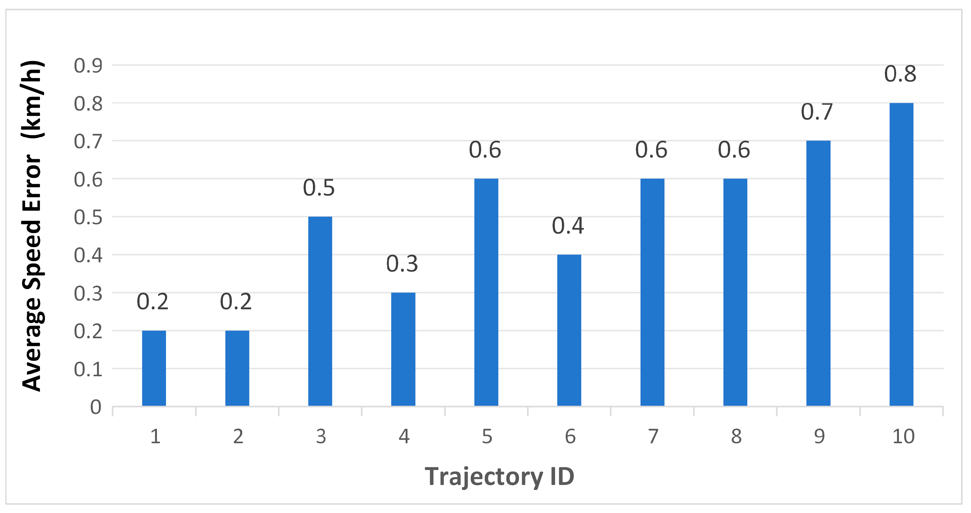
Trajectory ID	Duration (min)	Points	Fitted K	Synchronous Euclidean Distance (m)	Average Speed Error (km/h)
1	40	51	400	2.5	0.2
2	69	96	966	2.3	0.2
3	105	126	969	2.8	0.5
4	112	116	1311	3.3	0.3
5	179	240	1182	3.7	0.6
6	183	190	1903	3.8	0.4
7	225	300	1211	4.4	0.6
8	272	320	2000	4.2	0.6
9	308	310	1600	4.6	0.7
10	326	333	2011	4.5	0.8

shows the duration and points of each trajectory line. Figure 9 shows four trajectory lines (numbered a, b, c, and d) among them.

Based on the model and algorithm described above, the trajectory lines are fitted according to the following steps. The specific process is as follows:

• Supplementary feature points: Monitor the trajectory line according to the process of adding the key feature points shown in Figure 4, calculate the time and speed according to Formula (6) at the place where they need to be added, and generate new nodes and insert them into the trajectory line, so as to obtain the modified trajectory line containing the newly inserted nodes.
• Obtain the number of terms K in the Fourier expansion: Substitute the duration and points of the original discrete trajectory data into Formula (10) as input parameters to obtain the number of Fourier expansion terms K suitable for the duration and number of points.
• Obtain the amplitude array of harmonic components: Taking time as the independent variable, expand the original trajectory data within a given time span to K terms based on Formula (5) to obtain an amplitude array of harmonic components containing position and velocity information.
• Fitted trajectory points: Select an arbitrary time point (this time point must be within the time duration of the original trajectory), and together with the amplitude array, substitute this into Formula (4) for inverse Fourier transform to obtain the fitted position and velocity at the selected time point.

4.2. Result Analysis

After analyzing the selected trajectory data according to the fitting steps, the fitting K value, point fitting average deviation, and speed average deviation of 10 trajectory lines are finally obtained, which correspond to columns 4, 5, and 6 of Table 5, respectively. It is found that the deviation range of the synchronous Euclidean distance of 10 trajectory lines is within [2.3, 4.6] m, as shown in Figure 10, while the average error of fitting speed is in the range of [0.2, 0.8] m/s, as shown in Figure 11. According to the calculation with a scale of 1:40 k, the corresponding actual distance tolerance is 40 m. The point offset is significantly lower than the limit value. For speed fitting, the fitting error threshold is set to 1/10 of the original speed. The average range of the original velocity is within [12.3, 24.8] m/s, so the velocity fitting error threshold should be less than 1.2 m/s in theory. This shows that the actual velocity error is far below the theoretical error threshold. These quantitative calculation results show that the trajectory points and trajectory lines obtained by fitting fully meet the needs of visualization.

Figure 12 shows the comparison diagram of the offset before and after the fitting of the two trajectory lines (a) and (c) in Figure 9. From the local enlarged drawing, it can be seen that the fitting trajectory line is generally well fitted with the original trajectory line, maintaining the geometric accuracy of the original trajectory line. Most of the fitting trajectory points overlap with the original trajectory points, and a small proportion of them have a small offset, but they are all within the threshold range.

5. Comparison Between Fourier Fitting and Bézier Fitting of Trajectory Data

The Bézier curve is mainly used to describe smooth curves and is a mathematical curve widely used in computer graphics, animation, font design, and other fields. As a fitting method, the Bézier curve has multiple orders of expression. This article adopts the commonly used third-order Bézier curve expression [23], and its model is as follows:

$$B\left(t\right)=P_0{\left(1-t\right)}^3+P_1{\left(1-t\right)}^{2}t+P_2{\left(1-t\right)}^{2}t+P_3{t}^3$$

(11)

Among them, B$\left(t\right)=(X\left(t\right),Y\left(t\right))$. $t$ is a parameter whose value is the ratio of the duration from the starting point to the sampling point on the trajectory line to the total duration from the starting point to the endpoint. The value range of $t$ is [0, 1]. $P_0$, $P_1,$ $P_2$, and $P_3$ are the four control points of the Bézier curve, where $P_1$ and $P_2$ are the control points to be determined and the coordinates of $P_0$,$P_1{,P}_2$, and $P_3$ are $($X0, Y0$)$,$($X1, Y1$)$, $($X2, Y2$)$, and $($X3, Y3$)$, respectively. Under the condition of a scale of 1:40 K and using the same number of parameters, Fourier and Bézier fitting operations were performed on the four trajectory lines shown in Figure 9, and then the Fourier fitting curve, Bézier fitting curve, and original curve were superimposed for comparative analysis.

Table 6. A comparison of Fourier and Bézier fitting accuracy with the same number of parameters.

Trajectory ID	Fitting Algorithm	Number of Parameters Involved in Fitting
		400	600	800	1000	1200	1400
		Synchronous Euclidean Distance (m)
a	Fourier	58.1	24.4	19.1	5.6	2.7	1.8
	Bézier	46.1	47.4	78.1	102.9	120.9	140.8
b	Fourier	82.6	42.0	32.5	9.7	4.6	3.1
	Bézier	72.5	72.5	88.1	130.3	134.2	138.1
c	Fourier	106.2	50.6	39.6	11.5	5.4	3.4
	Bézier	48.8	49.1	84.5	113.6	130.6	143.5
d	Fourier	103.9	47.5	40.7	12.0	5.8	3.6
	Bézier	52.4	54.7	87.0	120.6	123.2	129.2

lists the fitting accuracy results of these two algorithms on four trajectory lines. Figure 13 compares and displays the two fitting effects of trajectory line d.

Table 6 shows that as the number of fitting parameters gradually increases from 400 to 1400, the synchronous Euclidean distance deviation range of Fourier fitting for trajectory lines a, b, c, and d decreases from the range of [58.1, 106.2] m to the range of [1.8, 3.6] m, with a significant decrease in deviation values and a significant improvement in fitting accuracy. The situation of Bézier fitting is exactly the opposite, with the synchronous Euclidean distance deviation range increasing from an interval of [46.1, 72.5] m to an interval of [129.2, 143.5] m, with a significant increase in deviation values and a significant decrease in fitting accuracy. As shown in Figure 13, the overall comparison and local magnification of the two fitted trajectory lines of trajectory line d with the original trajectory line indicates that the Fourier fitting curve highly overlaps with the original curve, basically reproducing the characteristics of the original curve, and the fitting effect is good. However, the Bézier fitting curve deviates significantly from the original curve both globally and locally, resulting in poor fitting performance.

Bézier fitting curves consist of multiple segmented curves [24], requiring separate functions to be stored in different intervals, which increases maintenance difficulty and query complexity. Under random sampling time points, searching for the fitted position value requires a full-line search, which is cumbersome and time-consuming. In contrast, the Fourier model uses a single periodic function to comprehensively describe the trajectory, simplifying storage and queries, allowing for direct acquisition of the fitted position value for any given sampling time point.

In terms of expressing the instantaneous speed of floating vehicles, the Fourier model demonstrates significant advantages. The Fourier function expresses both speed and position within the time interval, while the Bézier model is limited to position representation.

Table 7. The difference between the Fourier method and the Bézier method in modeling position and velocity.

Features	Fourier Method	Bézier Method
Modeling Object	Location and speed information	Only location information
Description Method	Frequency domain representation and periodic function	Control points and basis functions
Speed Modeling Capability	Capable of modeling speed changes	Cannot directly model speed
Location Modeling Capability	Suitable for describing periodic changes in location information, capable of capturing frequency components	More suitable for describing local position changes and boundary conditions
Application Scenarios	Signal processing, audio synthesis	Graphic interpolation, animation path
Computing Efficiency	Can efficiently process large-scale data	Computational complexity, especially in high-dimensional situations, makes parameter selection difficult and sensitive to boundary conditions
Robustness	Has good robustness to periodic noise data	Performs well for smooth changing physical phenomena, but is sensitive to noise
Flexibility	Can adapt to multiple frequency components, but performs poorly on nonperiodic signals	Specially designed for specific geometric shapes with limited flexibility

compares the Fourier and Bézier methods across multiple dimensions [25,26,27], with results showing that the Fourier method has a clear advantage in modeling position and speed, particularly in handling complex dynamic signals, offering higher accuracy and robustness. The Fourier model’s capability to analyze the frequency domain makes it widely applicable in signal processing, image, and audio analysis, while the Bézier method appears inadequate in dynamic signal modeling and complex path processing. Therefore, the Fourier method is generally preferred, especially in scenarios requiring high accuracy and dynamic response.

6. Discussion and Summary

Floating car trajectory data, characterized by their temporal, spatial, and diverse nature, have become a crucial foundation for transportation planning and travel demand forecasting. In recent years, the integration of trajectory data with emerging technologies has become increasingly close. Autonomous vehicles leverage large volumes of trajectory data to train algorithms, intelligent transportation systems monitor traffic conditions in real-time, and shared mobility platforms rely on user trajectories to optimize vehicle dispatching. Additionally, vehicle-to-everything (V2X) technology enables real-time data sharing between vehicles and infrastructure, while trajectory data generated in drone delivery operations aid in optimizing flight paths. However, floating car trajectories often exhibit irregular and dynamic changes, resulting in frequent stops and starts, which in turn generate numerous redundant points and jump points. Traditional methods struggle to accurately capture these patterns. While linear interpolation is widely used due to its simplicity and efficiency, it can lead to information loss under large sampling intervals, affecting the true characteristics of trajectories. Bézier curves and polynomial regression are suitable for handling simple trajectories, whereas spline and polynomial methods can address more complex local features. However, these methods are prone to noise interference in complex trajectory data, leading to poor fitting results and ineffective handling of redundant and jump points. Machine learning methods adapt to different data characteristics but suffer from poor interpretability due to their “black box” nature. Fourier methods excel in handling periodic data, enabling effective frequency domain analysis, with spectral analysis offering better interpretability and robustness against noisy data. By adjusting the number of terms in the Fourier series, one can flexibly meet different precision requirements. Furthermore, Fourier methods can convert discrete trajectory points into continuous curves, thereby enhancing the usability and analytical accuracy of trajectory data.

Although the Fourier model exhibits favorable characteristics in trajectory data analysis, the time consumed may significantly increase when dealing with long time series, large-scale data, and complex trajectories, thereby affecting the efficiency of practical applications. Therefore, it is necessary to explore more efficient algorithms, such as parallel computing or machine learning techniques, to accelerate the fitting process of Fourier series. Although Fourier models can improve fitting accuracy, it is still necessary to pay attention to the potential adverse effects of trajectory data duration, number of trajectory points, and their complexity on model performance. Adaptive adjustment mechanisms should be developed to dynamically regulate the number of Fourier expansion terms based on data characteristics, achieving optimal fitting results under different scenarios. Future research should focus on developing new metrics to quantify the shape information of geographic features, elucidating the relationship between shape information and spatial scale, and reasonably selecting the number of trajectory data points at different scales. Additionally, floating car trajectory data is often combined with other data sources (e.g., traffic flow, meteorological information, etc.), and how to effectively integrate multi-source data to enhance comprehensive analytical capabilities remains an important research topic. Future efforts should explore multi-modal data fusion methods, leveraging machine learning and deep learning techniques to extract valuable information from multiple data sources, thereby improving the accuracy of travel demand prediction and the scientific nature of traffic planning.

A floating car trajectory analysis method based on road network structure and Fourier series fitting demonstrates significant advantages in handling irregular and dynamically changing trajectory data. Compared to traditional analysis methods, this technique excels in addressing information gaps and data noise while also achieving notable improvements in precision and continuity. However, future research must focus on key challenges such as computational efficiency, fitting accuracy, quantification of geometric features, and integration of multi-source data to facilitate the widespread application of this method in intelligent transportation systems and travel demand forecasting. These studies will provide more reliable and precise data support for transportation decision-making.

References

- Zhu, Q.; Fu, X. The Review of Visual Analysis Methods of Multi-modal Spatio-temporal Big Data. Acta Geod. Cartogr. Sin. 2017, 46, 1672–1677. [Google Scholar]
- Draper, N.; Smith, H. Applied Regression Analysis, 3rd ed.; John Wiley & Sons: New York, NY, USA, 1998; pp. 15–96. [Google Scholar]
- Powell, M. Approximation Theory and Methods; Cambridge University Press: New York, NY, USA, 1981; pp. 33–41. [Google Scholar]
- De Boor, C. A Practical Guide to Splines; Springer: New York, NY, USA, 1978; pp. 2–15. [Google Scholar]
- Loader, C. Local Regression and Likelihood; Springer: New York, NY, USA, 1999; pp. 15–76. [Google Scholar]
- Smola, A.J.; Schölkopf, B. A tutorial on support vector regression. Stat. Comput. 2004, 14, 199–222. [Google Scholar] [CrossRef]
- Journel, A.; Huijbregts, C. Mining Geostatistics; Academic Press: London, UK, 1978; pp. 25–130. [Google Scholar]
- Anselin, L. Local indicators of spatial association—LISA. Geogr. Anal. 1995, 27, 93–115. [Google Scholar] [CrossRef]
- Jolliffe, I.T. Principal component analysis: A beginner’s guide—I. Introduction and application. Weather 1990, 45, 375–382. [Google Scholar] [CrossRef]
- Anselin, L. Spatial Econometrics: Methods and Models; Springer Science & Business Media Dordrecht: Berlin, Germany, 1988; pp. 16–115. [Google Scholar]
- Wu, H.H. Study of Mathematical Model for Fitting S shape Distributed Data. Geomat. Inf. Sci. Wuhan Univ. 2009, 4, 474–478. [Google Scholar]
- Douglas, D.H.; Peucker, T.K. Algorithms for the reduction of the number of points required to represent a digitized line or its caricature. Cartogr. Int. J. Geogr. Inf. Geovisualization 1973, 10, 112–122. [Google Scholar] [CrossRef]
- Li, Z.L.; Openshaw, S. Algorithms for automated line generalization based on a natural principle of objective generalization. Int. J. Geogr. Inf. Syst. 1992, 6, 373–389. [Google Scholar] [CrossRef]
- Bi, J.; Zhu, Y.; Cheng, Y. A Comprehensive Map Matching Algorithm Based on Curve Fitting and Network Topology. J. Transp. Inf. Saf. 2014, 32, 127–131. [Google Scholar]
- Yang, M.; Chen, Y.Y.; Jin, C.; Cheng, Q. A Method of Speed-preserving Trajectory Simplification. Acta Geod. Cartogr. Sin. 2017, 46, 2016–2023. [Google Scholar]
- Wu, J.G.; Liu, M.; Wei, G.; Liu, L.F. An Improved Trajectory Data Compression Algorithm of Sliding Window. Comput. Technol. Dev. 2015, 25, 47–51. [Google Scholar]
- Ai, T.H.; Shuai, Y.; Li, J.Z. A Spatial Query Based on Shape Similarity Cognition. Acta Geod. Cartogr. Sin. 2009, 38, 356–362. [Google Scholar]
- Shuai, Y.; Ai, T.H.; Shuai, H.Y.; Ni, L. Polygonal Inquiry Based on Shape Template Matching. Geomat. Inf. Sci. Wuhan Univ. 2008, 33, 1267–1270. [Google Scholar]
- Liu, P.C.; Ai, T.H. Applications of Shape Recognition in Map Generalization. Acta Geod. Cartogr. Sin. 2012, 41, 316. [Google Scholar]
- Liu, P.C.; Ai, T.H.; Bi, X. Multi-scale Representation Model for Contour Based on Fourier Series. Geomat. Inf. Sci. Wuhan Univ. 2013, 38, 221–224. [Google Scholar]
- Liu, P.C.; Xiao, T.Y.; Xiao, J.; Ai, T.H. A multi-scale representation Model of Polyline Based on Head/Tail Breaks. Int. J. Geogr. Inf. Sci. 2020, 34, 2275–2295. [Google Scholar] [CrossRef]
- Xiang, L.G.; Gong, J.Y.; Wu, T.; Li, W.H. Spatio-Temporal Trajectory Relationships Based on Stop/Move Abstraction. Geomat. Inf. Sci. Wuhan Univ. 2014, 39, 956–962. [Google Scholar]
- Li, J.C.; Zhao, D.B. An Investigation on Image Compression Using the Trigonometric Bézier Curve with a Shape Parame ter. Math. Probl. Eng. 2013. [Google Scholar] [CrossRef]
- Sarfraz, M.; Asim, M.R.; Masood, A. Capturing outlines using cubic Bezier curves. In Proceedings of the 2004 International Conference on Information and Communication Technologies, Bangkok, Thailand, 3–5 November 2004; IEEE: Damascus, Syria, 2004; pp. 539–540. [Google Scholar]
- Liu, P.C.; Ma, H.R.; Zou, Y.; Shao, Z.Q. Autoencoder neural network method for curve data compression. Acta Geod. Cartogr. Sin. 2024, 53, 1634–1643. [Google Scholar]
- Heckbert, P. Fourier transforms and the fast Fourier transform (FFT) algorithm. Comput. Graph. 1995, 2, 15–463. [Google Scholar]
- Khan, K. Generalized Bézier Curves and Their Applications in Computer Aided Geometric Design. Ph.D. Dissertation, Jawaharlal Nehru University New Delhi, New Delhi, India, 15 July 2018. [Google Scholar]