GeoFAN: Point Pattern Recognition in Spatial Vector Data

Abstract

The recognition of point patterns in spatial vector data has important applications in geographic mapping and formation recognition. However, the application of traditional methods to spatial vector data faces two difficulties. Firstly, these data are low signal-to-noise ratio data in which the point patterns are mixed with a large number of normal point clusters; thus, it is difficult to recognize point patterns from these unstructured data using traditional clustering or machine learning methods. Secondly, the lack of edge connectivity relationships in spatial vector data directly hinders the application of graph models. Few studies have systematically solved the above difficulties. In this article, we propose a geometric feature attention scheme to overcome the above challenges. We also present an implementation of the scheme based on the graph method, termed GeoFAN, to extract and classify point patterns simultaneously in spatial vector data. Firstly, the raw data are transformed into a graph structure consisting of adjacency and attribute matrices. Secondly, a geometric feature attention module is proposed to enhance the feature representation of point patterns. Finally, the recognition results of all points are output via GeoFAN. The macro precision, recall, and $F_1$ score of five simulated point pattern types with different attributes and point numbers are 92.8%, 90.3%, and 91.5%, respectively, and GeoFAN is trained with simulated data to recognize real location-based point patterns successfully. The proposed GeoFAN showed superior performance and generalization ability in point pattern recognition.

1. Introduction

Point pattern recognition in spatial vector point data refers to the automatic recognition of interested point clusters with spatial distribution characteristics, including artificial elements such as building clusters, aircraft and ship formations, and natural elements such as island clusters and river systems. In geographic mapping, point pattern recognition enhances the description of regional geographic features by mining the principal components in space, thus reflecting important geographic features [1,2]. In formation recognition, point pattern recognition discovers battle formations among a large number of points, thus enhancing regional situational awareness and helping safeguard regional rights and interests [3,4,5].

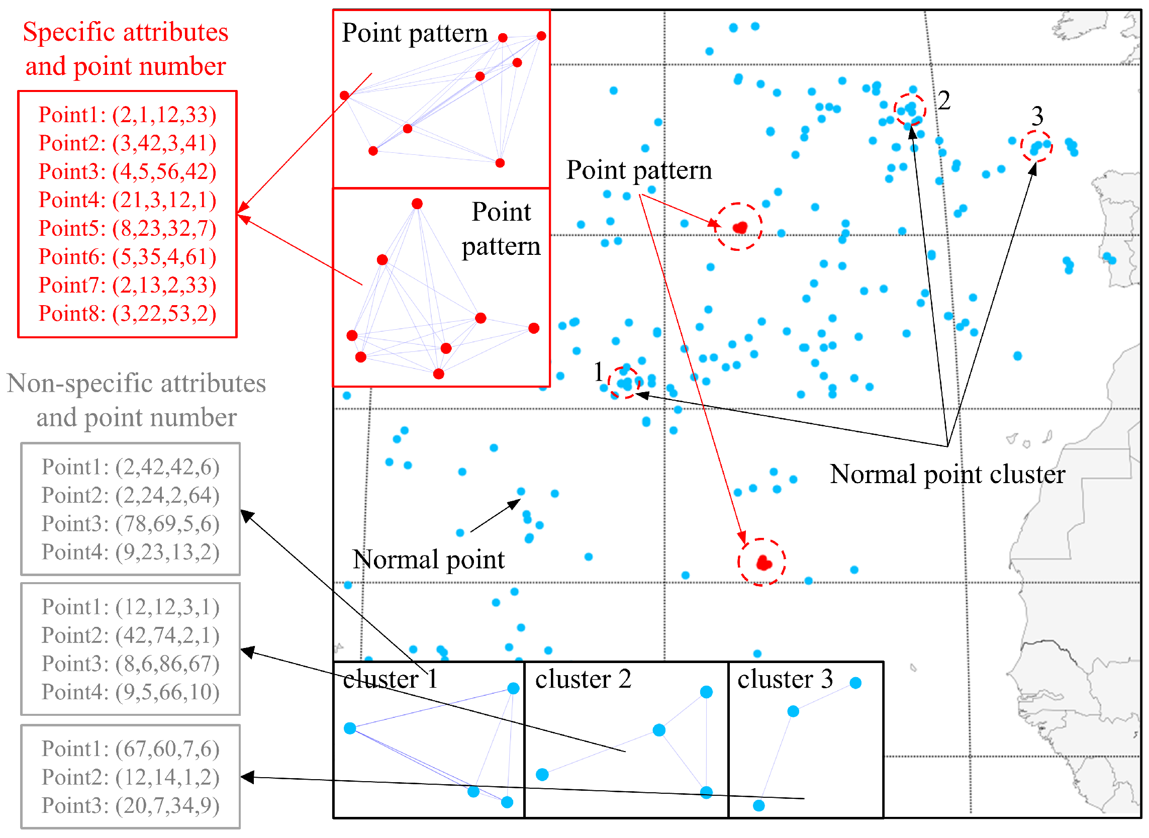
Due to the complexity and specificity of spatial vector data, the current point pattern recognition process is usually extracted first and then classified, which is difficult to complete at one time. The complexity is that these data have low signal-to-noise ratio (SNR), uneven spatial distribution [6,7], and point pattern diversity [8], as shown in Figure 1. The point patterns are mixed with normal points and normal point clusters, which can easily lead to misclassification by traditional clustering or machine learning methods. The specificity is that the distribution of points in spatial vector data has complex non-Euclidean features, and it is difficult to model its attribute and spatial correlation directly by traditional methods. In comparison, the graph-based method expresses the coupling between attributes and space explicitly through the adjacency and attribute matrices, which is a direct and efficient way to represent the spatial vector data. However, spatial vector data contain only point locations without edge relationships [9]; it is necessary to construct the adjacency matrix artificially [10]. The geometric features of the data are as important as the point attributes [11], which, together, constitute the fingerprint of the point pattern. Although the distance threshold parameter can be used to determine neighbors, it results in the initial distance weights of all neighboring nodes being equalized (e.g., binarized 0/1 connections) if only this aggregation condition is used, thus losing the geometric features that are implied by the actual distance differences. In addition, the choice of the threshold parameter presents subjective difficulties. If the threshold is chosen too large, it leads to the aggregation of false targets, and if the threshold is chosen too small, it leads to disconnection within the point pattern. Techniques such as inverse distance weighting and radial basis functions can assign different weights to neighboring points. However, existing research lacks models based on inverse distance weighting or radial basis functions in the integration of point pattern extraction and classification applications.

In earlier studies, point pattern extraction was achieved by designing multiple spatial constraints to delineate point clusters progressively. Basaraner et al. delineate building clusters by strong geospatial separation of elements such as roads, rivers, etc. [12]. However, methods that simply rely on other elements to achieve clustering struggle to obtain more detailed results, and elements used for delineation are often lacking in practical situations. Point clustering methods have been introduced to point pattern extraction for their simplicity [13]. These methods combine the points that satisfy the conditions into new clusters through homogeneity constraints, mostly derived from classical point clustering algorithms, including the K-Means algorithm [14], the DBSCAN algorithm [15], etc. In [16], a Gaussian kernel-based DBSCAN method is introduced to extract ship formations under different clutter ratios efficiently. Cetinkaya et al. compared the effectiveness of four algorithms for grouping buildings, of which DBSCAN performs better in grouping buildings in urban blocks with different distributions [17]. Graph theory has also been applied to point clustering. Yan et al. used multidimensional features of buildings as node attributes, input the spectral domain graph convolutional neural network to predict the center location coordinates of clusters, and used the K-Means method to cluster the buildings [18]. Point pattern recognition methods based on clustering algorithms can simply and quickly extract the point pattern with aggregated distribution. However, they need to set the artificial parameter, which increases application difficulty, and is prone to false extraction when the SNR is low and there are normal point clusters. Other extraction methods, such as neighborhood graph-based methods (e.g., Delaunay Triangulation (DT), Nearest Neighbor Graph (NNG), Minimum Spanning Tree (MST), etc.), are overly dependent on expert experience and difficult to generalize [19,20,21,22].

To classify the extracted point patterns, template matching-based methods were developed [23,24]. They classify point patterns by comparing them with standard templates. In [25], a Hough transform-based method for classifying ship formations is introduced. It detects formation shapes such as straight lines formed by ships through the Hough transform and then compares them with templates to realize ship formation recognition. Cheng et al. processed the binary coded mapping using the convolutional Radon transform and compared formations with three standard templates, classifying “Y”, “T”, and “I” ship formations with different offsets [26]. The logic of the template-based method is simple. However, template matching methods will fail if the point pattern is partially obscured or slightly deviates from the template.

Machine learning methods make point pattern classification intelligent. He et al. proposed a depthwise separable convolutional neural network (DSCNN) to classify ship formations with different point detection errors [16]. Lin et al. proposed the Long Short-Term Memory (LSTM)-based algorithm for aircraft formation classification [27]. Liang et al. designed a formation coding method and combined it with a support vector machine (SVM) to construct a formation recognition model with 0.955 recognition accuracy [28]. A CNN-based aircraft formation recognition method is later proposed, with an improved recognition accuracy of 0.965 [29]. He et al. classified the clustered building patterns using the random forest algorithm and further partitioned the building clusters with no recognized patterns based on the graph partitioning method [30]. Machine learning has received much attention since it can automatically mine data for features. However, spatial vector data have unstructured properties; thus, traditional machine learning methods struggle to capture complex structural information from them.

Traditional methods that simply concatenate point attributes and spatial coordinates limit the ability to deeply integrate heterogeneous information, such as spatial proximity and semantic features. In comparison, graph neural networks (GNNs) can jointly process spatial positions and attribute features by constructing spatial proximity networks. Lin et al. introduced a recognition algorithm based on a graph neural network and the LSTM network to recognize ship formations [31]. Yan et al. classified regular and irregular building patterns using a graph convolutional neural network [32]. Scholars extend the applications of GNN by transforming some scenarios into point pattern recognition problems. In [33], a model that combines the Shape Context (SC) descriptor and a graph convolutional neural network (GCNN) is proposed to classify the interchange patterns. Yu et al. modeled river systems as graph structures and proposed a river system pattern recognition algorithm based on a spectral domain graph convolutional neural network to classify river systems [34]. GNN has significant advantages when working with non-Euclidean data. It requires an adjacency matrix as input. However, since spatial vector data contain only point locations without edge information, GNN cannot be directly applied. Although it is possible to construct the adjacency matrix by setting the aggregation condition, the geometric features of the graph may be lost, and the aggregation condition is cumbersome to set up. Inverse distance weighting and radial basis functions can assign different weights to neighboring points without setting an aggregation condition. However, existing research lacks relevant models directly applied to integrated point pattern extraction–classification scenarios.

Table 1. Advantages and disadvantages of different methods in spatial vector point pattern recognition.

Approaches		Advantages	Disadvantages
Point pattern extraction	Segmentation elements	Utilizes natural/artificial elements for pattern separation with intuitive logic.	Highly dependent on auxiliary geographic elements.
	Clustering	Simple and efficient for large-scale data; effective for explicit spatial aggregation patterns.	Require manual parameter tuning; vulnerable to noise/normal clusters in low-SNR scenarios.
	Neighborhood graph	Pattern separation through spatial proximity in the absence of segmentation elements.	Dependent on expert experience; difficult to generalize.
Point pattern classification	Template matching	Simple matching logic; high accuracy for standardized point pattern classification.	Partially obscured or small deviation from the template may result in a match failure.
	Traditional machine learning	Automatically learn the features in the sample that have been extracted to achieve the extraction of the unknown point pattern.	Difficulty in capturing spatial correlation of unstructured data.
	Graph neural network	Explicit spatial-attribute coupling via graph structures; handles non-Euclidean data.	Cannot be applied directly in space vector data due to lack of adjacency matrices.

summarizes the strengths and weaknesses of existing methods in spatial vector point pattern recognition. The traditional point pattern extraction methods based on clustering algorithms face the difficulty of artificial parameter adjustment and low-SNR scenario application. Point pattern classification methods based on template matching and traditional machine learning are difficult to apply in complex scenarios. Graph methods cannot be applied directly due to the lack of edge information. In this article, we propose a graph structure of spatial vector data and a GEOmetric Feature Attention Network (GeoFAN) for point pattern recognition in spatial vector data.

Our main contributions are as follows:

1.

A graph conversion method for raw spatial vector data is proposed to represent the spatial distribution and attributes of all points. The distance between points is calculated as weighted adjacency matrices. The point characteristics are used as attribute matrices to realize the graph conversion, which fully expresses the geometric feature of the raw data. Complete and accurate data conversion is the basis of point pattern recognition.

2.

A geometric feature attention scheme is proposed to enhance the features of point patterns. The scheme can embed the graph geometric features in the attention coefficients and achieve the global weighted aggregation, which avoids setting up the aggregation conditions and solves the problem that the graph neural network cannot be directly applied to spatial vector data. As the geometric features of the spatial vector data are fully utilized, the differences between patterned points and normal points and between different point patterns are increased, which solves the difficulty of the low-SNR scenario application.

3.

A GeoFAN method is proposed to recognize point patterns in low-SNR spatial vector data. It solves the difficulty that extraction and classification cannot be done simultaneously, and it is a general and effective method to recognize point patterns in spatial vector data without setting any artificial parameters. The method is tested and evaluated by simulated point patterns and real location-based point patterns with different patterned point spacing, domain area range (no other points exist within this range of a point pattern), and point pattern types. The test results show that GeoFAN has superior recognition performance and generalization ability in point pattern recognition scenarios.

The rest of the article is organized as follows. Section 2 describes the materials and methods. Section 3 presents the experimental results. Section 4 discusses the findings and future work. Section 5 concludes the article.

2. Materials and Methods

In this section, we study the graph conversion of spatial vector data and the point pattern recognition method. Spatial vector data consists of points’ latitude, longitude, and attributes. By converting raw spatial vector data into a graph structure consisting of adjacency matrices and attribute matrices, the spatial distribution characteristics and point attributes can be extracted to express the raw spatial vector data effectively. Then, we propose a GeoFAN point pattern recognition method. The inputs are the adjacency and attribute matrices of the graph data, and the outputs are the point classification results numbered by point pattern types. We outline the structure of GeoFAN and describe in detail the point pattern recognition procedure.

2.1. Spatial Vector Data Graph Conversion

2.1.1. Raw Spatial Vector Data

Typically, observation instruments are located far from the targets to obtain spatial vector data from a wide area. Therefore, the effect of elevation can be ignored, and the observation area forms a two-dimensional plane.

An example of raw spatial vector data is shown in Figure 1. The data can be decomposed as follows:

1.

Point set: $\mathbf{V}\in {\mathbb{R}}^{n\times 1}$

2.

Latitude and longitude set: $\mathbf{P}\in {\mathbb{R}}^{n\times 2}$. The latitude and longitude in radians of the ith point are denoted as ${\mathbf{p}}_i=({\phi }_i,{\lambda }_i)$

3.

Attribute set: $\mathbf{X}\in {\mathbb{R}}^{n\times d}$. The attributes of the ith point are denoted as ${\mathbf{x}}_i=(x_{i1},x_{i2},\cdots ,x_{id})$

2.1.2. Graph Conversion

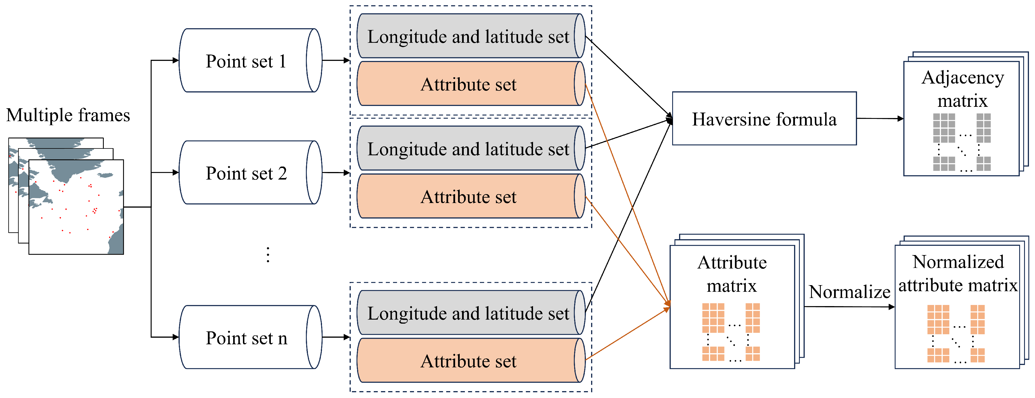
A complete graph includes the adjacency matrix $\mathbf{A}$ and the attribute matrix $\mathbf{X}$. In this section, we construct the adjacency matrix of the spatial vector data by the relative distance between points and the attribute matrix by the characteristics of all points. The conversion procedure is shown in Figure 2.

In spatial vector data, the points consist of normal and patterned points. Patterned points tend to be more aggregated and characterized by relative spatial proximity; thus, pairs of points with smaller spatial distances are more likely to be associated. To obtain spatial distance information, we calculate the relative spatial distance between points by latitude and longitude. If the data do not have latitude and longitude information, other methods are used to calculate the relative spatial distance.

The haversine formula is an effective method for calculating distances based on the difference in latitude and longitude between two points on the Earth, which is widely used in geographic information systems. The haversine formula for calculating the distance between two points is as follows:

$$a_{ij}=2Rarcsin\left(\sqrt{H\left(\mathrm{\Delta }\phi \right)+cos\left({\phi }_i\right)cos\left({\phi }_j\right)H\left(\mathrm{\Delta }\lambda \right)}\right)$$

(1)

$$H\left(\theta \right)={sin}^2\left({\displaystyle \frac{\theta }{2}}\right)$$

(2)

$$\mathrm{\Delta }\phi ={\phi }_j-{\phi }_i$$

(3)

$$\mathrm{\Delta }\lambda ={\lambda }_j-{\lambda }_i$$

(4)

where H is the haversine function. $a_{ij}$ is the spatial distance between the ith point and the jth point. R is the radius of the Earth.

The distance-weighted adjacency matrix $\mathbf{A}$ can be obtained by calculating the haversine formula.

The point characteristics obtained from the spatial vector data contain multiple parameters. We assumed that the points in the raw spatial vector data contain three parameters, such as length, width, and height. Since the instrument has observation errors and points’ parameters may be time-varying, each parameter has maximum, minimum, and average values. The attribute matrix can be constructed as $\mathbf{X}\in {\mathbb{R}}^{n\times 9}$, and its row vector ${\mathbf{x}}_i$ is the attribute vector of the ith point:

$$\begin{array}{c}\hfill {\mathbf{x}}_i=(x_{i1},x_{i2},x_{i3},x_{i4},x_{i5},x_{i6},x_{i7},x_{i8},x_{i9})\end{array}$$

(5)

where $x_{i1}$, $x_{i2}$, and $x_{i3}$ are the maximum, average, and minimum values of the 1st parameter of the ith point, respectively. $x_{i4}$, $x_{i5}$, and $x_{i6}$ are the maximum, average, and minimum values of the 2nd parameter of the ith point, respectively. $x_{i7}$, $x_{i8}$, and $x_{i9}$ are the maximum, average, and minimum values of the 3rd parameter of the ith point, respectively.

To make different attributes have the same weight, we normalize the columns of the attribute matrix to obtain the normalized attribute matrix $\overline{\mathbf{X}}$:

$$m_j=\underset{i}{max}{x}_{ij}$$

(6)

$${\overline{x}}_{ij}={\displaystyle \frac{x_{ij}}{m_j}}$$

(7)

where $m_j$ is the maximum value of the jth column of the attribute matrix $\mathbf{X}$. ${\overline{x}}_{ij}$ is the element of the ith row and the jth column of the normalized attribute matrix $\overline{\mathbf{X}}$.

2.2. Recognize Point Pattern via GeoFAN

2.2.1. Geometric Feature Attention Module

The graph neural network is an effective method for processing spatial vector data. With the development of graph neural networks, a variety of models, such as the graph convolutional network (GCN), graph autoencoder (GAE), graph generative network (GGN), graph recurrent network (GRN), and graph attention network (GAT), have appeared. These models can be adapted to multiple types of tasks at the node, edge, and graph levels.

Spatial vector data have the following characteristics. There are far more normal points in a frame than point patterns. Normal points are unevenly distributed, and some have stronger aggregation characteristics than point patterns. The strong similarity of different point patterns makes them difficult to distinguish. The above issues make point pattern recognition more challenging. Attention mechanisms can effectively face the above challenges, and they have been widely used in deep neural networks. They can enhance the model’s extraction performance of key features from the data and improve its expressive ability by adaptively assigning weights to different neighbors, thus achieving more accurate recognition results.

We calculate the correlation coefficient of the point pairs from the attributes of the points. The correlation matrix $\mathbf{E}$ can be represented as

$$e_{ij}=\sigma ({\mathbf{x}}_i,{\mathbf{x}}_j)$$

(8)

where $e_{ij}$ is the element of the ith row and the jth column of the correlation matrix $\mathbf{E}$. ${\mathbf{x}}_i$ is the attribute vector of the ith point. ${\mathbf{x}}_j$ is the attribute vector of the jth point. $\sigma (·)$ is a function that calculates the correlation of two points.

We choose a single fully connected layer to represent $\sigma (·)$. The correlation coefficient can be represented as

$$e_{ij}=\mathrm{LeakyRelu}\left([{\mathbf{x}}_i\mathbf{W}\parallel {\mathbf{x}}_j\mathbf{W}]{\mathbf{u}}^T\right)$$

(9)

where ‖ is a column-splicing operation. $\mathbf{W}\in {\mathbb{R}}^{d\times d_1}$ is the downscale conversion matrix of the point attribute of the trainable fully connected layer. $\mathbf{u}\in {\mathbb{R}}^{2d_1}$ is the weight vector of the layer. We select the activation function with reference to [35], the activation function is LeakyReLU (negative slope is 0.2), thereby introducing a nonlinear capability to the network.

The correlation coefficients are calculated between all points, including the coefficient of each point with itself. According to Equation (9), the correlation matrix $\mathbf{E}$ can be obtained by inputting the point attributes.

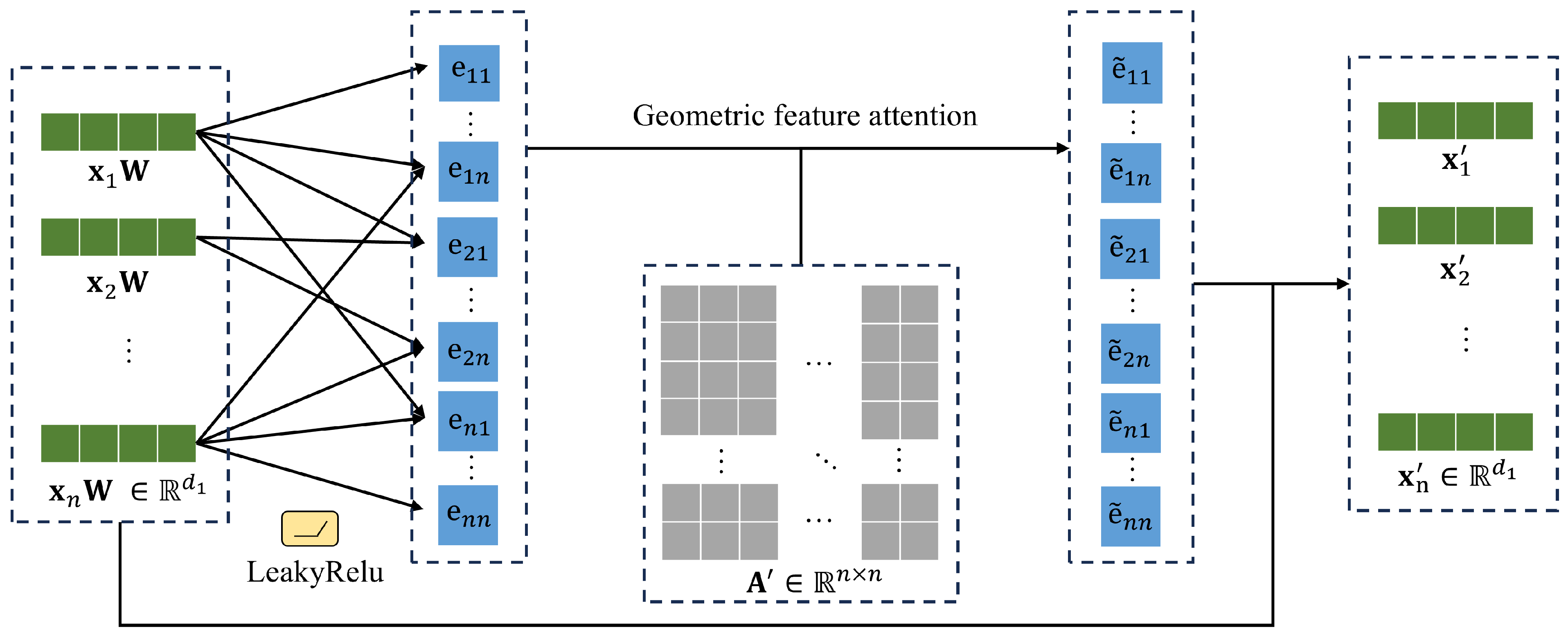
To enhance the features of point patterns, a geometric feature graph attention (GeoFA) mechanism is proposed, as shown in Figure 3. Taking the inverse of all elements in the adjacency matrix $\mathbf{A}$ and multiplying them with the corresponding elements in the correlation matrix $\mathbf{E}$ to obtain the geometric feature attention matrix $\tilde{\mathbf{E}}$,

$$a_{ij}^{\prime }=1/a_{ij}$$

(10)

$${\tilde{e}}_{ij}=a_{ij}^{\prime }{e}_{ij}$$

(11)

where ${\tilde{e}}_{ij}$ is the element of the ith row and the jth column of the geometric feature attention matrix $\tilde{\mathbf{E}}$.

The geometric feature attention module enables points with closer spatial distances to have greater weights, resulting in relatively greater attention coefficients, enhancing the difference between patterned and normal points. After calculating the geometric feature attention coefficients, the aggregation operation is realized, and the new attribute vector of point $v_i$ can be output:

$${\mathbf{x}}_i^{\prime }=\sum _{j=1}^n{\tilde{e}}_{ij}{\mathbf{x}}_j\mathbf{W}$$

(12)

The above describes the single-head geometric feature attention module.

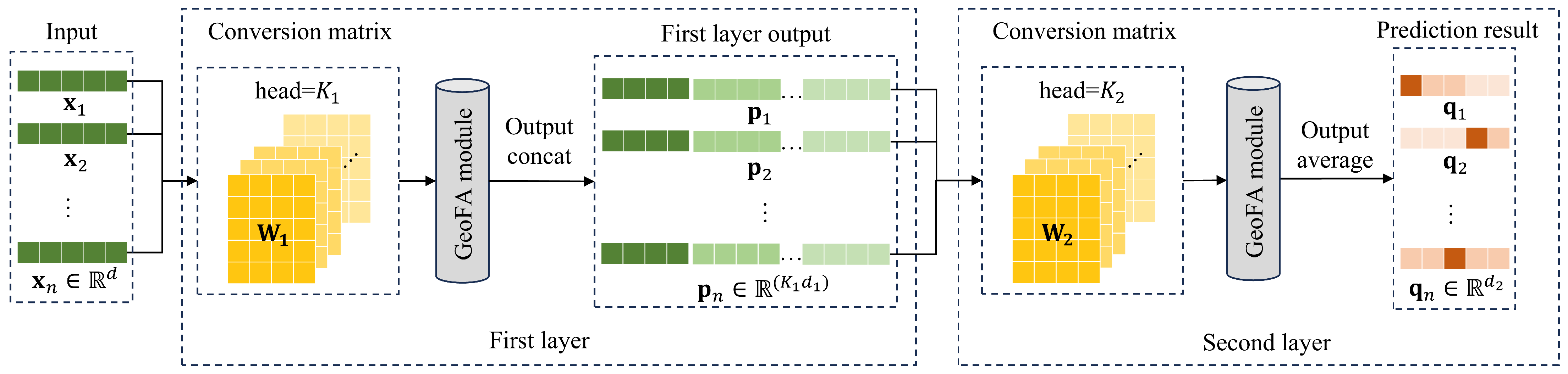
2.2.2. Structure of GeoFAN

To further enhance the expressive power of the attention layer, a multi-head attention mechanism is introduced. K mutually independent attention modules are invoked, and the output of each module is then spliced together. A graph attention network layer can be represented as

$${\mathbf{x}}_i^{\prime \left(k\right)}=\sum _{j=1}^n{\tilde{e}}_{ij}^{\left(k\right)}{\mathbf{x}}_j{\mathbf{W}}^{\left(k\right)}$$

(13)

where ${\tilde{e}}_{ij}^{\left(k\right)}$ is the geometric feature attention coefficient calculated by the kth GeoFA module between the ith and the jth point. ${\mathbf{W}}^{\left(k\right)}$ is the conversion matrix of the point attributes of the kth GeoFA module.

By adding multiple independent attention modules, the model can allocate attention to multiple relevant features between the center point and neighboring points, which enhances the model’s learning ability. The structure of the proposed GeoFAN method is shown in Figure 4. We used two multi-head graph attention layers to map the attribute network in low dimensions. The output of each GeoFA module in the first layer is obtained by splicing, and the output of each GeoFA module in the second layer is averaged to obtain the prediction results. The first layer output ${\mathbf{p}}_i$ and the second layer output ${\mathbf{q}}_i$ of the ith point are represented as follows:

$${\mathbf{p}}_i={\left|\right|}_{k=1}^{K_1}\sum _{j=1}^n{\tilde{e}}_{i{j}_1}^{\left(k\right)}{\mathbf{x}}_j{\mathbf{W}}_1^{\left(k\right)}$$

(14)

$${\tilde{e}}_{i{j}_1}^{\left(k\right)}={\displaystyle \frac{1}{a_{ij}}}\mathrm{LeakyRelu}\left(\right[{\mathbf{x}}_i{\mathbf{W}}_1^{\left(k\right)}\left|\right|{\mathbf{x}}_j{\mathbf{W}}_1^{\left(k\right)}\left]{\mathbf{u}}_1^T\right)$$

(15)

$${\mathbf{q}}_i={\displaystyle \frac{1}{K_2}}\sum _{k=1}^{K_2}\sum _{j=1}^n{\tilde{e}}_{i{j}_2}^{\left(k\right)}{\mathbf{p}}_j{\mathbf{W}}_2^{\left(k\right)}$$

(16)

$${\tilde{e}}_{i{j}_2}^{\left(k\right)}={\displaystyle \frac{1}{a_{ij}}}\mathrm{LeakyRelu}\left(\right[{\mathbf{p}}_i{\mathbf{W}}_2^{\left(k\right)}\left|\right|{\mathbf{p}}_j{\mathbf{W}}_2^{\left(k\right)}\left]{\mathbf{u}}_2^T\right)$$

(17)

where ${\mathbf{W}}_1^{\left(k\right)}\in {\mathbb{R}}^{d\times d_1}$ is the point attribute conversion matrix of the first layer of GeoFAN, used to map the input attribute matrix $\mathbf{X}$ from d-dimensional to $d_1$-dimensional. The attribute vector of the ith point output by the first layer is ${\mathbf{p}}_i\in {\mathbb{R}}^{\left(K_1{d}_1\right)}$. ${\mathbf{W}}_2^{\left(k\right)}\in {\mathbb{R}}^{\left(K_1{d}_1\right)\times d_2}$ is the point attribute conversion matrix of the second layer of GeoFAN. The attribute vector of the ith point output by the second layer is ${\mathbf{q}}_i\in {\mathbb{R}}^{d_2}$.

The GeoFAN outputs the probability that each point belongs to each type; thus, its column dimension is equal to the number of point types. After taking the type with the largest probability as the recognition result of each point, point pattern recognition is realized.

2.3. Experimental Data and Environment

To validate the effectiveness of our proposed method, we performed qualitative and quantitative assessments of point pattern recognition effects. We constructed a formation recognition scenario. The experiment datasets in the article are synthetic datasets of 242 frames to simulate the satellite observation scenarios of ships at sea, the coordinates of ships in the synthetic datasets are extracted from the global satellite Automatic Identification System (AIS) data in 2016 to simulate the real spatial distribution of the ships, the study area covers the global major shipping lanes and sea areas, and the attributes are artificially generated, which are not directly mapped to the real physical parameters, focusing on verifying the model’s ability to mine point patterns with arbitrary features. The average point number of each frame is 264. Each point has specific attributes, realizing the construction of the spatial vector datasets.

The point attributes contain three main types of parameters: $x_1$, $x_2$, and $x_3$. In practical scenarios, such as electromagnetic satellite signal detection, the target attributes contain the maximum, minimum, and average values of the signal during the observation time, with the maximum/minimum reflecting the fluctuating range of the signal attribute, and the average reflecting the signal attribute under its steady-state operation, which together define the fingerprint of the target. However, due to the sparsity of the actual data and the lack of a priori knowledge of the target, the true average value distribution is difficult to predict. To simulate the randomness of average values in real scenarios and ensure the generalization ability of the model under limited data, we selected nine parameters: $x_{1\max }$, $x_{1\mathrm{ave}}$, $x_{1\min }$, $x_{2\max }$, $x_{2\mathrm{ave}}$, $x_{2\min }$, $x_{3\max }$, $x_{3\mathrm{ave}}$, and $x_{3\min }$. The statistical parameters we set for all the points are shown in Figure 5. The average values of three parameters are randomly generated were between the maximum and minimum values to cover all possible average values in real scenarios.

There are a large number of normal points and only 0–3 point patterns in a single frame in the datasets, resulting in an average SNR lower than 5%. To make the model learn more point pattern features, data expansion is needed to increase the richness of the training datasets. Different numbers of point patterns were added to each frame, expanding the 242 datasets to 1000, significantly increasing the training data for learning. The training and test datasets were divided in a 9:1 ratio. Please note that the point patterns added to the datasets were only used for simulated analysis. In the real location-based point pattern recognition scenario, the datasets are not expanded.

The training was performed with Python 3.9. We trained our model using PyTorch 1.9.0 on NVIDIA GeForce RTX 2060. Since the patterned points in the datasets were fewer than normal points, the learning rate was too high to recognize all points as normal points, and too low to converge too slowly. We set the initial learning rate to 0.003, and after every 1 epoch, the learning rate was reduced to 0.997. The attention heads of both geometric feature attention layers were set to 8. The training process was stopped when the loss was no longer decreasing to prevent overfitting. In our datasets where there were more negative samples and fewer positive samples, we used three metrics to accurately and comprehensively evaluate the recognition effect of the GeoFAN method: macro accuracy, macro recall, and macro $F_1$ score:

$$MacroP={\displaystyle \frac{1}{m}}\sum _{i=1}^m{P}_i$$

(18)

$$MacroR={\displaystyle \frac{1}{m}}\sum _{i=1}^m{R}_i$$

(19)

$$Macro{F}_1={\displaystyle \frac{1}{m}}\sum _{i=1}^m{F}_{1i}$$

(20)

$$F_{1i}={\displaystyle \frac{2\times P_i\times R_i}{P_i+R_i}}$$

(21)

where m denotes the classes of points. $P_i$ denotes the precision of the ith label. $R_i$ denotes the recall of the ith label. $F_{1i}$ denotes the $F_1$ score of the ith label. Macro-metrics can give the same weight to positive and negative samples, thus effectively evaluating the model’s recognition performance.

3. Results

In this section, we test the recognition performance of GeoFAN using synthetic datasets. The effects of patterned point spacing, domain area range, and point pattern types on the recognition performance are analyzed, respectively, and we designed experiments to compare GeoFAN with other algorithms. The effectiveness of GeoFAN in point pattern recognition is verified by applying the method to real location-based points.

3.1. Performance Under Various Patterned Point Spacing

To analyze the model’s recognition effect under different patterned point spacing, we expanded the datasets by adding point patterns with different point spacing to the original point background.

Firstly, we set the condition that the maximum patterned point spacing is smaller than 100 km, then randomly selected a point cluster from the synthetic datasets that satisfies the condition as a point pattern, and used its point number and the attributes of each point as the fingerprint of this point pattern type. Multiple point pattern types could be generated according to the same method. Then, we obtained the latitude and longitude range of point distribution in each frame, randomly generated the center points of point patterns within this range, and generated the patterned points near each center point. By controlling the maximum spacing of patterned points, we created point patterns with different patterned point spacing. The following constraints were used to control the patterned point spacing:

$$d_{\max }\le L_{\lim }$$

(22)

where $d_{\max }$ represents the maximum distance between points in a point pattern. $L_{\lim }$ represents the constraint distance.

We used the original datasets as background and added patterned points with a maximum spacing of 20 km, 40 km, 60 km, 80 km, and 100 km as five different recognition scenarios. The 242 datasets were expanded to 1000 in each scenario. The point pattern type was 1. The attributes of the generated point patterns are shown in

Table 2. Attributes of each point in the point pattern.

Point Index	${\mathit{x}}_1$		${\mathit{x}}_2$		${\mathit{x}}_3$
	Max	Min	Max	Min	Max	Min
1	86.29	86.20	16.68	16.61	1.12	1.08
2	51.72	46.52	29.62	16.38	6.58	1.52
3	45.23	44.39	48.61	13.62	6.51	1.02
4	82.02	81.99	28.27	25.38	1.20	1.09
5	44.92	44.30	26.67	9.50	9.74	0.96
6	51.42	46.52	17.30	8.92	4.33	3.06
7	43.54	43.39	50.74	13.04	6.61	6.06
8	13.67	13.41	23.69	16.94	32.54	31.50

. Point index 1–8 indicates that this specific point pattern contains exactly 8 points. The number of point patterns in each frame is 0–6. The domain area range is 50 km. $x_{1\mathrm{ave}}$, $x_{2\mathrm{ave}}$, and $x_{3\mathrm{ave}}$ are randomized between the minimum and maximum values.

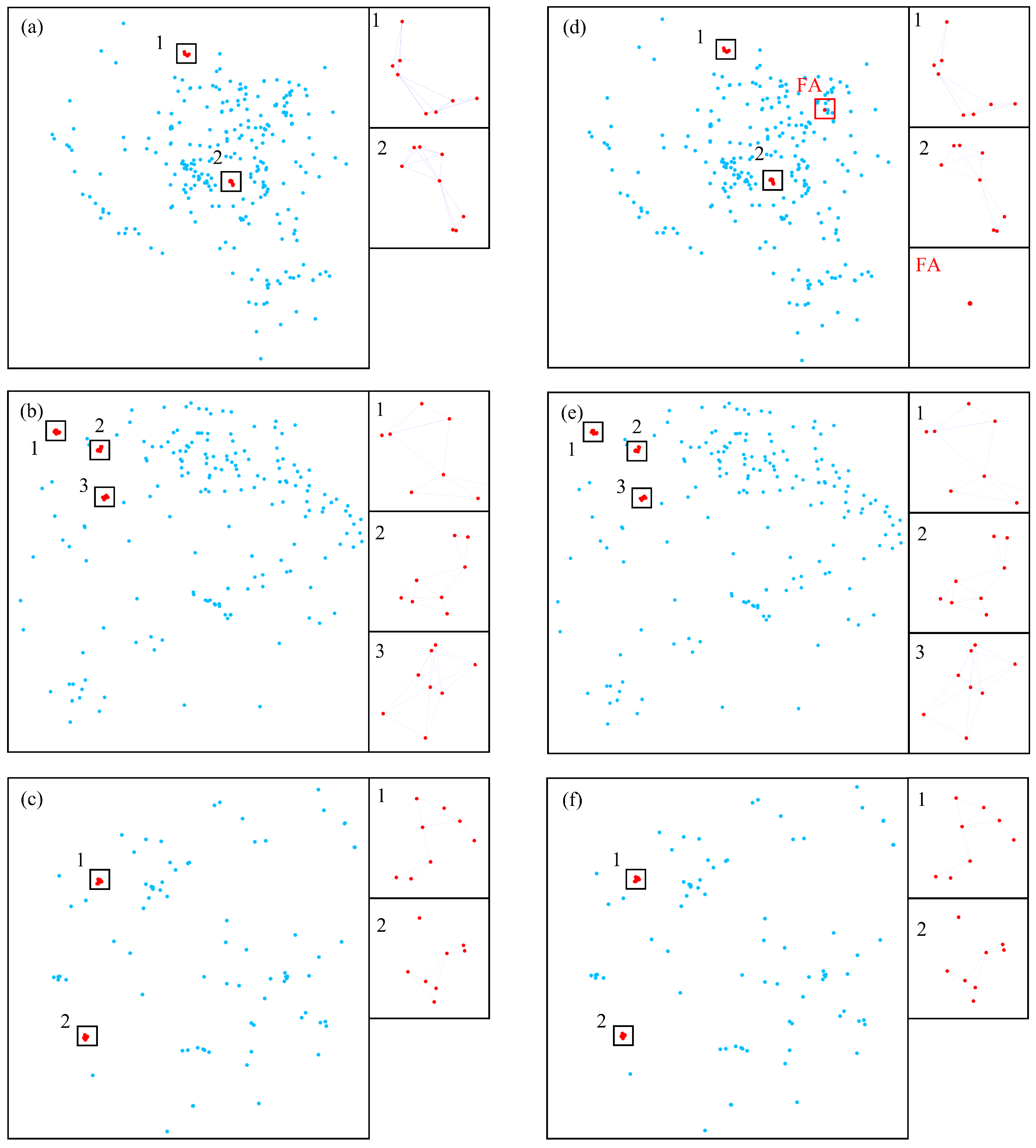
The recognition results of three frames of the maximum spacing of 100 km are shown in Figure 6. Figure 6a–c show the ground truth of three frames. Figure 6d–f show the recognition results of the three frames. From the results, it can be seen that there are a few false alarms in Figure 6d. Figure 6e,f show that the recognition results of the second and third frames are consistent with the ground truth, which shows that GeoFAN has good recognition ability for point patterns with a maximum patterned point spacing of up to 100 km.

The precision, recall, and $F_1$ score results are shown in

Table 3. Precision, recall, and $F_1$ score (%) of different maximum patterned point spacings.

Point Type	20 km			40 km			60 km			80 km			100 km
	$\mathit{P}$	$\mathit{R}$	${\mathit{F}}_{\mathbf{1}}$	$\mathit{P}$	$\mathit{R}$	${\mathit{F}}_{\mathbf{1}}$	$\mathit{P}$	$\mathit{R}$	${\mathit{F}}_{\mathbf{1}}$	$\mathit{P}$	$\mathit{R}$	${\mathit{F}}_{\mathbf{1}}$	$\mathit{P}$	$\mathit{R}$	${\mathit{F}}_{\mathbf{1}}$
Normal	99.84	99.81	99.83	99.55	99.74	99.65	99.68	99.37	99.53	99.25	99.53	99.39	98.87	99.45	99.21
Patterned	97.79	98.18	97.99	96.83	94.67	95.74	93.04	96.42	94.70	95.01	92.31	93.64	93.86	88.93	91.33
Macro	98.82	99.00	98.91	98.19	97.20	97.69	96.36	97.89	97.11	97.13	95.92	96.52	96.41	94.19	95.27

. It shows that the proposed GeoFAN performs better in recognizing point patterns with smaller point spacing than with larger point spacing. When the maximum patterned point spacing is small, the attention coefficients of patterned points will be larger than those of normal points after being weighted by the distance, increasing the difference of their updated attribute vectors. When the maximum patterned point spacing is large, the attention coefficient between points in point patterns decreases, thus the patterned points and normal points have strong similarity in updated attribute vectors, making it difficult for the model to differentiate between normal points and patterned points, thus the recognition effect of the model decreases.

3.2. Performance Under Various Domain Area Ranges

In geographic mapping and formation recognition, point patterns usually exhibit spatial independence in spatial vector data, i.e., they are spatially distant from other points, and this distance is referred to as the domain area range. Within the domain area range of point patterns, it can be assumed that there are no other points. In the original point background, we added point patterns with different domain area ranges of 100 km, 400 km, 700 km, and 1000 km as four different recognition scenarios. The 242 datasets were expanded to 1000 in each scenario. The point pattern attributes are the same as in Table 2. The maximum patterned point spacing was 100 km. The point pattern type was 1. The number of point patterns in each frame was 0–6.

The recognition results are shown in

Table 4. Precision, recall, and $F_1$ score (%) of different domain area ranges.

Point Type	100 km			400 km			700 km			1000 km
	$\mathit{P}$	$\mathit{R}$	${\mathit{F}}_{\mathbf{1}}$	$\mathit{P}$	$\mathit{R}$	${\mathit{F}}_{\mathbf{1}}$	$\mathit{P}$	$\mathit{R}$	${\mathit{F}}_{\mathbf{1}}$	$\mathit{P}$	$\mathit{R}$	${\mathit{F}}_{\mathbf{1}}$
Normal	99.06	99.36	99.21	98.98	99.47	99.23	99.01	99.50	99.25	99.42	99.61	99.52
Patterned	92.92	89.85	91.36	94.38	89.58	91.92	95.58	91.50	93.50	96.28	94.53	95.40
Macro	95.99	94.61	95.28	96.68	94.53	95.57	97.29	95.50	96.38	97.85	97.07	97.46

. The test results show that the GeoFAN method better recognizes point patterns with a larger domain area range than those with a smaller domain area range. When the domain area range is small, the normal points spatially close to the patterned points have large attention coefficients, which increases the difficulty of model recognition, resulting in the normal points being misclassified as patterned points. When the domain area range is larger, the number of normal points near the patterned points are reduced, including some “normal point clusters” with aggregation characteristics (see Figure 1), which increases the SNR of the datasets and the difference between the attention coefficients of the patterned points and the normal points. Therefore, the patterned points’ recognition accuracy, recall, and $F_1$ score are improved.

3.3. Performance Comparison with Clustering Algorithm

We specifically added comparison experiments on the classical DBSCAN clustering algorithm and GeoFAN, since only a single point pattern type is involved in Section 3.1 and Section 3.2 (essentially, the detection of spatially aggregated clusters). To verify the key role of attributes in pattern recognition, the experiments were designed in two typical scenarios: scenario A (maximum patterned point spacing of 100 km, domain area range of 50 km) and scenario B (maximum patterned point spacing of 100 km, domain area range of 100 km), which maintain a correspondence with the experimental conditions of Section 3.1 and Section 3.2. Considering the sensitivity of the DBSCAN algorithm to parameter settings, we used parameter optimization seeking on the entire dataset to confirm optimal parameters and perform point pattern extraction with these parameters.

Table 5. Performance comparison with DBSCAN on point pattern extraction.

Point Type		DBSCAN			Ours
		$\mathit{P}$	$\mathit{R}$	${\mathit{F}}_{\mathbf{1}}$	$\mathit{P}$	$\mathit{R}$	${\mathit{F}}_{\mathbf{1}}$
Maximum patterned point spacing of 100 km	Normal	96.52	99.03	97.76	98.87	99.45	99.21
	Patterned	70.23	89.64	78.76	93.86	88.93	91.33
	Macro	83.38	94.34	88.26	96.41	94.19	95.27
Domain area range of 100 km	Normal	96.62	99.23	97.90	99.06	99.36	99.21
	Patterned	71.20	91.74	80.18	92.92	89.85	91.36
	Macro	83.91	95.49	89.04	95.99	94.61	95.28

shows the performance comparison results of the two algorithms in the two scenarios.

The experimental results show that GeoFAN achieves macro $F_1$ scores of 95.27% and 95.28% in the two test scenarios, which are higher than those of 88.26% and 89.04% for DBSCAN. The main reason is that DBSCAN only relies on spatial features for extraction, and is prone to misjudge normal point clusters with aggregation characteristics as patterned points in low-SNR scenarios, which is reflected in its low precision. In comparison, GeoFAN achieves the synergistic processing of spatial proximity and attributes through the geometric feature attention mechanism, which effectively constructs the joint spatial-attribute fingerprints of the point patterns, mitigating the misclassification of normal point clusters. It is worth noting that the weak advantage of DBSCAN in the recall index reveals the difference between the two algorithms: DBSCAN captures more normal point clusters with dense distribution, and has fewer misses compared to GeoFAN. Since the point patterns in the training datasets have fewer point pattern samples compared to normal points, there is a category imbalance; thus, GeoFAN may omit some patterned points.

In practice, the performance of DBSCAN relies on manual parameter tuning and only enables pattern extraction, not classification. GeoFAN not only circumvents the artificial parameter tuning problem through the end-to-end learning paradigm, but also realizes the integrated extraction–classification processing, which is fully verified in the following experiments with various pattern types.

3.4. Performance Under Various Point Pattern Types

The definition of point pattern type includes both point number characteristics and attribute characteristics, and two point patterns are considered to be of different types when they differ in either of these two characteristics. In the original point background, multiple types of point patterns were added to verify the ability of GeoFAN. The point pattern types for the four scenarios were 2, 3, 4, and 5, respectively. The 242 datasets were expanded to 1000 in each scenario. The attributes of the first type are listed in Table 2, and the attributes of the remaining four types of point patterns are shown in

Table 6. Attributes of each point in the second type of point pattern.

Point Index	${\mathit{x}}_1$		${\mathit{x}}_2$		${\mathit{x}}_3$
	Max	Min	Max	Min	Max	Min
1	42.42	42.27	29.27	21.47	1.58	1.52
2	79.70	79.61	77.13	76.94	2.38	2.25
3	80.19	80.01	47.69	47.64	2.22	2.20
4	49.20	49.13	22.88	20.91	14.63	14.53
5	15.49	15.35	67.69	65.36	2.89	0.72
6	82.79	82.66	8.56	8.08	599.8	9.36

,

Table 7. Attributes of each point in the third type of point pattern.

Point Index	${\mathit{x}}_1$		${\mathit{x}}_2$		${\mathit{x}}_3$
	Max	Min	Max	Min	Max	Min
1	83.81	83.80	124.99	124.91	12.41	11.85
2	81.22	81.11	125.03	124.92	0.27	0.21
3	83.89	83.81	125.06	124.81	0.53	0.24
4	41.67	41.44	21.46	16.40	1.46	0.27
5	45.71	45.67	35.77	31.20	1.14	1.08

,

Table 8. Attributes of each point in the fourth type of point pattern.

Point Index	${\mathit{x}}_1$		${\mathit{x}}_2$		${\mathit{x}}_3$
	Max	Min	Max	Min	Max	Min
1	54.06	38.94	20.08	19.94	1.36	1.18
2	49.61	47.40	59.62	8.02	3.52	1.61
3	45.14	44.22	192.37	16.10	3.33	0.92
4	13.69	13.53	23.62	16.99	31.95	31.77
5	16.40	16.29	182.27	18.00	0.61	0.51
6	51.51	46.49	12.99	8.08	6.68	1.22
7	83.75	83.63	17.51	15.70	0.41	0.30
8	82.02	81.97	28.03	25.10	1.53	1.04
9	52.46	51.71	31.96	9.83	3.46	3.39

and

Table 9. Attributes of each point in the fifth type of point pattern.

Point Index	${\mathit{x}}_1$		${\mathit{x}}_2$		${\mathit{x}}_3$
	Max	Min	Max	Min	Max	Min
1	85.18	83.67	17.63	15.74	0.61	0.25
2	82.02	81.98	28.51	24.83	1.27	1.10
3	45.05	44.33	53.19	14.90	6.44	0.84
4	51.66	46.57	12.23	7.11	3.47	1.38
5	13.57	13.47	23.60	17.41	31.97	31.84
6	52.39	51.74	18.39	5.90	3.46	3.28

. The maximum patterned point spacing was 60 km. The domain area range was 50 km. In the four scenarios, the numbers of point patterns in each frame were 0–12, 0–18, 0–24, and 0–30, respectively, to ensure the balance of point pattern number of each type in different scenarios.

The recognition results are shown in

Table 10. Precision, recall, and $F_1$ score (%) of different point pattern types.

Point Type	2 Types			3 Types			4 Types			5 Types
	$\mathit{P}$	$\mathit{R}$	${\mathit{F}}_{\mathbf{1}}$	$\mathit{P}$	$\mathit{R}$	${\mathit{F}}_{\mathbf{1}}$	$\mathit{P}$	$\mathit{R}$	${\mathit{F}}_{\mathbf{1}}$	$\mathit{P}$	$\mathit{R}$	${\mathit{F}}_{\mathbf{1}}$
Normal	99.29	99.43	99.36	98.93	98.80	98.86	98.00	99.16	98.58	98.14	99.21	98.67
1st Pattern	94.70	93.04	93.86	90.58	98.28	94.27	93.10	90.07	91.56	86.22	88.10	87.15
2nd Pattern	98.67	98.91	98.79	98.91	97.56	98.23	98.24	98.62	98.43	96.57	96.22	96.40
3rd Pattern	-	-	-	93.79	85.67	89.55	95.09	85.70	90.15	96.07	87.41	91.53
4th Pattern	-	-	-	-	-	-	96.85	93.37	95.08	95.53	95.94	95.73
5th Pattern	-	-	-	-	-	-	-	-	-	84.34	74.91	79.35
Macro	97.55	97.13	97.34	95.55	95.08	95.23	96.26	93.38	94.76	92.81	90.30	91.47

. When the point pattern types increase from 2 to 4, the precision, recall, and $F_1$ scores of different types do not change significantly. However, when adding the fifth type, the recognition effect of the first and fifth types decrease, while the recognition effect of the other types is not affected much. This is because the newly added type has a very strong similarity to the first type. Point indexes 1, 2, 3, 5, and 6 of the fifth type are similar to point indexes 1, 4, 3, 8, and 6 of the first type. With such a strong similarity, it is difficult to distinguish between the two point pattern types. Nevertheless, the GeoFAN model still captures the minor attribute differences and point number differences between the two types, with $F_1$ scores of 87.15% and 79.35% for the two point pattern types, respectively, verifying the robustness and effectiveness of GeoFAN in point pattern recognition. The recognition results illustrate that the number of types does not significantly affect the recognition results, while similar point patterns will.

In the scenario of five point pattern types, we compared the recognition performance of the graph convolutional network (GCN), 1-neighbor graph attention network (1N-GAT), and 2-neighbor graph attention network (2N-GAT) with our proposed GeoFAN. Due to the lack of adjacency information in the raw spatial vector data, GAT could not be directly applied to our scenarios and required the artificial construction of adjacency matrices. We improved GAT to 1N-GAT and 2N-GAT. 1N-GAT and 2N-GAT represent the graph attention networks aggregating one and two nearest neighbor points, respectively. 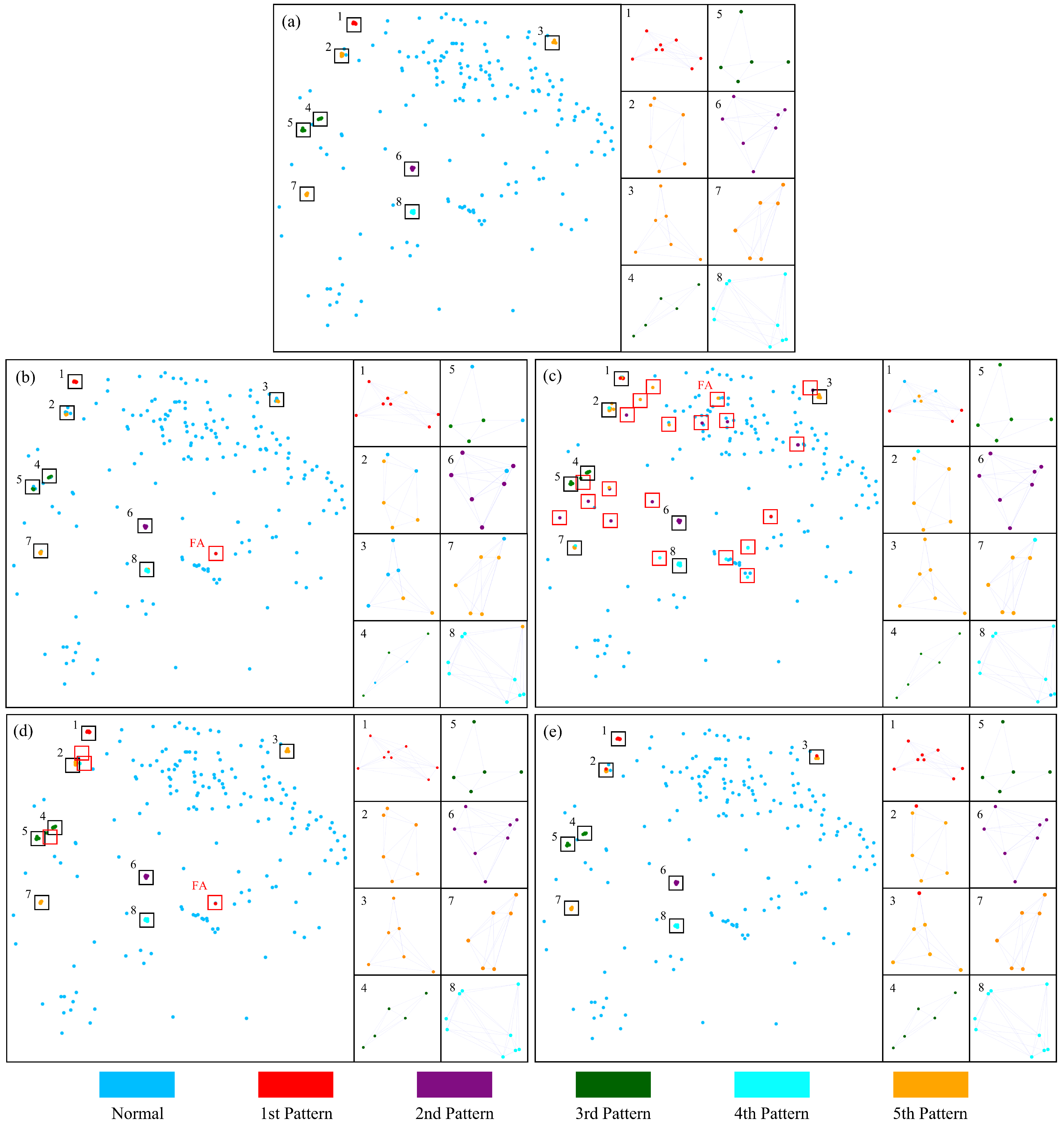Figure 7 demonstrates a frame of recognition results of GCN, 1N-GAT, 2N-GAT, and GeoFAN. Figure 7a is the ground truth of this frame. As shown in Figure 7b, there are more misclassifications and omissions in the GCN recognition result, which may be caused by the difficulty of GCN in capturing neighboring features. 1N-GAT may cause normal points to be misclassified as patterned points because it only aggregates one nearest neighbor of each point, and many false alarms (FAs) can be seen in Figure 7c. In Figure 7d, 2N-GAT aggregates two nearest neighbors and achieves a better result than 1N-GAT, and still, FAs exist. It shows that increasing the number of aggregated nearest neighbors can reduce FAs. However, the number of aggregated neighbors can’t exceed point number in a single point pattern, otherwise the normal points will be aggregated incorrectly. Due to the variable point number in a point pattern, it is difficult to determine the number of neighbors that need to be aggregated in practical applications. In Figure 7e, although the GeoFAN recognizes a few points of the fifth type as the first type due to the similar attributes, there is no false alarm in the recognition result.

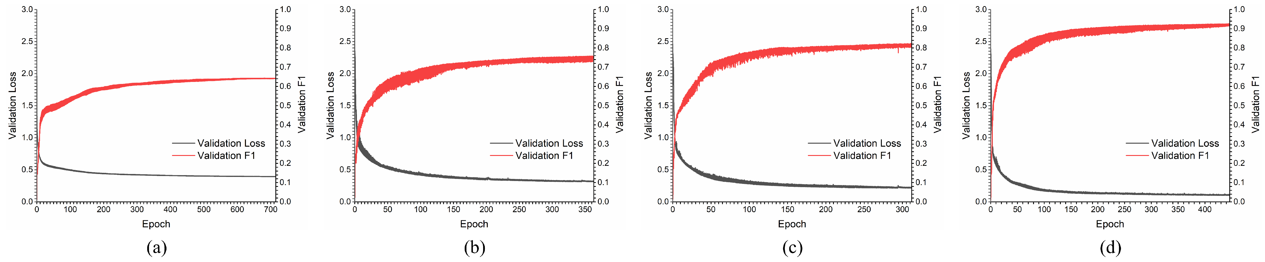
Figure 8 shows the training processes of the four algorithms in the scenario of five types, which are stopped when the losses do not decrease further. As seen from the training processes, our proposed GeoFAN model finally converges with a higher $F_1$ score of 0.915 than GCN 0.631, 1N-GAT 0.738, and 2N-GAT 0.786, and with a smaller loss value than the other three algorithms, which illustrates that the GeoFAN outperforms the GCN, 1N-GAT, and 2N-GAT in point pattern recognition. A comparison of the recognition performance of the four algorithms is shown in

Table 11. Comparison of the effectiveness of four algorithms in recognizing five point pattern types.

Point Type	GCN			1N-GAT			2N-GAT			Ours
	$\mathit{P}$	$\mathit{R}$	${\mathit{F}}_{\mathbf{1}}$	$\mathit{P}$	$\mathit{R}$	${\mathit{F}}_{\mathbf{1}}$	$\mathit{P}$	$\mathit{R}$	${\mathit{F}}_{\mathbf{1}}$	$\mathit{P}$	$\mathit{R}$	${\mathit{F}}_{\mathbf{1}}$
Normal	92.70	97.22	94.91	93.72	96.86	95.26	95.68	97.32	96.49	98.14	99.21	98.67
1st Pattern	64.71	57.23	60.74	61.92	68.98	65.26	66.00	72.22	68.97	86.22	88.10	87.15
2nd Pattern	74.41	67.23	70.64	86.02	76.37	80.91	89.66	87.47	88.55	96.57	96.22	96.40
3rd Pattern	79.18	51.95	62.74	91.91	77.29	83.97	88.28	86.12	87.19	96.07	87.41	91.53
4th Pattern	70.01	58.19	63.55	69.73	58.43	63.58	82.07	70.40	75.79	95.53	95.94	95.73
5th Pattern	40.66	18.98	25.88	58.64	49.55	53.71	58.48	50.84	54.39	84.34	74.91	79.35
Macro	70.28	58.47	63.08	76.99	71.25	73.78	80.03	77.40	78.56	92.81	90.30	91.47

, which indicates that GeoFAN performs better than other algorithms on all metrics for five types of point patterns.

The following may be the reason why the performance of other methods is limited. GCN is less flexible since the inter-node attribute correlation is not considered during the aggregation process, making it difficult to extract the correlation strength between the central node and its neighboring nodes in point patterns. 1N-GAT and 2N-GAT achieve better results than GCN by aggregating one and two nearest neighbor points around each point. However, due to the uneven distribution of points in point patterns, selecting too few points in the aggregation may lead to inter-disconnection. Although this can be mitigated by increasing the neighbor number used for aggregation, the point numbers of point patterns are variable; thus, the selection of the neighbor number used for aggregation is a great difficulty. In comparison, GeoFAN not only achieved better results, but also does not need to set artificial parameters, which is a practical and high-performance point pattern recognizer.

3.5. Performance Under Real Location-Based Point Patterns

The GeoFAN model has achieved excellent recognition performance in simulated point patterns. In practice, there may be a lack of training datasets of some point patterns, resulting in the model being unable to learn these point pattern types directly. Therefore, we use the GeoFAN model trained on simulated data to recognize the real location-based point patterns. This application can help recognize point patterns with sparse training datasets and predefine the unknown point patterns to be recognized.

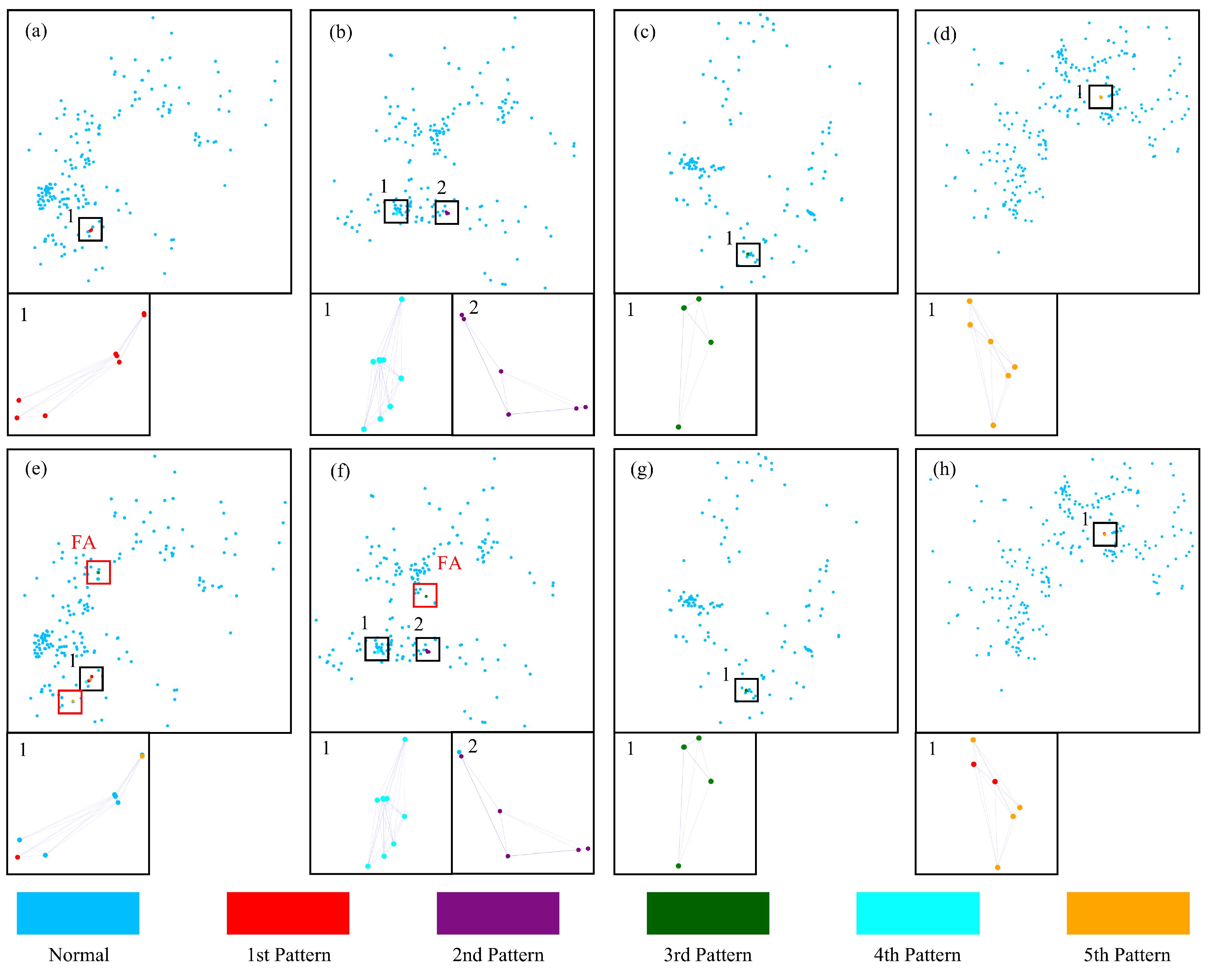
The method was applied to five different types of point patterns. Figure 9a–d show the ground truth of the five point pattern types in four frames. Figure 9e–h show the GeoFAN’s recognition results of the five point pattern types. From the recognition results, it can be seen that GeoFAN can accurately recognize the third and fourth types, as shown in Figure 9f,g. In Figure 9f, there is a slight misjudgment for the second type. Figure 9e,h show that recognition errors occur in the results of the first type and the fifth type. The recognition accuracies of the first and fifth types are affected by the similarity of their attributes, leading to crosstalk. Despite the crosstalk in the recognition results, the first and fifth types are not recognized as the other types. It illustrates that when two point patterns are very similar, correctly distinguishing between the two real point patterns using simulated data remains a huge challenge. Nevertheless, the GeoFAN still succeeds in separating the first type and the fifth type from the others and accurately recognizes some points on both types. The recognition results show that the GeoFAN model can be trained with simulated data to recognize real location-based point patterns, which is of high value in practical situations where there is a lack of point pattern datasets. GeoFAN recognizes multiple types of real location-based point patterns from a large number of points, which reaffirms the excellent performance of GeoFAN in low-SNR point pattern recognition scenarios.

4. Discussion

The GeoFAN framework proposed in this study effectively solves the dual challenges of low SNR and missing edge information, realizing point pattern recognition from spatial vector data through the fusion of the geometric feature attention mechanism and graph neural network. The method can realize simultaneous extraction and classification of point patterns without manual parameter tuning, which significantly improves the recognition accuracy of cluster structures (e.g., building and island clusters) in geographic mapping, and provides fast situational awareness for formation recognition (e.g., ship and aircraft formations). Its performance of successfully migrating to real location-based scenarios after training based on simulated data verifies the strong generalization ability of the model in scenarios where annotated data are scarce or expensive to acquire. This result provides a new paradigm for the automated analysis of complex spatial vector data, which is especially applicable to field that needs to mine weakly correlated patterns from massive, noisy data.

The joint spatial-attribute modeling mechanism designed in this study is similar to the idea of Tobler’s First Law, which is to increase the relevance of targets through their proximity. The inverse distance weighting first achieves the quantitative modeling of spatial proximity, effectively preserving spatial features’ continuity and integrity. Then, the geometric attention mechanism deeply integrates the spatial proximity and attribute correlation. This spatial-attribute coupled modeling mechanism shows advantages in the experiments, with the macro $F_1$ scores improving by 17.69% and 12.91% compared with 1N-GAT and 2N-GAT based on lossy spatial features and attributes, respectively, and the macro $F_1$ score improving by 6.24% compared with the DBSCAN based on spatial features. The core innovation is that GeoFAN not only retains the spatial features completely through inverse distance weighting, but also constructs a joint fingerprint of spatial proximity and attribute, which not only improves the effect compared to 1N-GAT, 2N-GAT, and DBSCAN, but also eliminates the need for manual parameter tuning and achieves the integration of extraction and classification.

The computational complexity of GeoFAN mainly involves two links. The feature mapping link maps all the node features from d-dimensional to $d_1$-dimensional, with a computational complexity of $O(n\times d\times d_1)$. The computation of attention link maps the $2d_1$ vectors of the paired points to the real numbers, and there are n points in a graph; thus, its computational complexity is $O(n^2\times d_1)$. The computational complexity of single-head GeoFAN is $O(n\times d\times d_1+n^2\times d_1)$. In our experiments, the average number of points in a single frame is about 264, and the model training and inference times are within an acceptable range at this scale. However, we observe increased video memory footprint and computation time when working with larger datasets ($n>264$). To address this problem, the following optimization strategies can be adopted: (1) A sparse attention mechanism. Constrain the global attention computation to the local neighborhood through K-nearest neighbor filtering, which reduces the complexity to $O\left(nK\right)$. (2) Hierarchical processing methods. Filter regions through density-awareness, then compute in the candidate regions. The above methods can significantly improve the computational efficiency while maintaining the performance of the model.

While GeoFAN performs well in point pattern recognition scenarios, distinguishing subtle distinctions among highly similar point patterns presents an opportunity for further refinement. In the future, a hybrid architecture combining attention and contrastive learning can be explored to strengthen the inter-class feature difference. In addition, it is necessary to integrate multimodal data to improve the performance of the point pattern recognition model. Finally, an incremental learning process can be introduced to realize the learning and recognition of unknown point patterns.

5. Conclusions

This article focuses on the problem of spatial vector point pattern recognition, proposing a graph conversion method for converting points based on latitude and longitude coordinates into a graph structure and a GeoFAN recognition model for point pattern recognition. The raw spatial vector data are converted into a graph structure through the inter-point distance and attributes, which are used as the input of the GeoFAN model. A geometric feature attention mechanism is proposed to enhance the inter-correlation of point patterns, and finally, the GeoFAN model effectively and accurately recognizes point patterns from the low-SNR spatial vector data. The experimental results show that GeoFAN can recognize the point patterns with five different types with a macro $F_1$ score of 91.47%, and it can recognize the real location-based point patterns by the model trained on the simulated data. In military scenarios, GeoFAN can identify high-threat battle formations based on satellite observation of ship positioning and attribute data, providing key decision-making support for battlefield situational awareness; in urban planning scenarios, GeoFAN can automatically identify building cluster patterns with specific spatial distribution and functional/structural characteristics, providing a basis for urban functional zoning and spatial structure optimization.

In subsequent work, we plan to introduce contrastive learning strategies to improve GeoFAN to recognize more similar point patterns, then include more types of point patterns for model training. Further, developing an incremental learning framework to enable continuous recognition of emerging point patterns will fill a critical technology gap in real-time spatial vector data analysis.