Article

Synergistic Mechanisms Between Elderly Oriented Community Activity Space Morphology and Microclimate Performance: An Integrated Learning and Multi-Objective Optimization Approach

by
Fang Wen
,
Lu Zhang
,
Ling Jiang
,
Rui Tang
and
Bo Zhang
*
School of Architecture and Art, North China University of Technology, Beijing 100144, China
*
Author to whom correspondence should be addressed.
These authors contributed equally to this article and should be regarded as co-first authors.
ISPRS Int. J. Geo-Inf. 2025, 14(6), 211; https://doi.org/10.3390/ijgi14060211
Submission received: 5 April 2025 / Revised: 11 May 2025 / Accepted: 20 May 2025 / Published: 28 May 2025

Abstract

:
This study collected site and spatial morphological data from 63 typical aging community activity spaces and extracted 12 spatial types through statistical analysis. A parametric modeling tool was used to generate spatial models. Based on clearly defined design variables and constraints, the NSGA-II multi-objective optimization algorithm was applied to minimize summer thermal discomfort, maximize winter thermal comfort, and maximize annual average sunlight duration, resulting in 342 Pareto optimal solutions. The study first explored the linear relationships between spatial morphology and environmental performance using the Spearman method. It then integrated ensemble learning and the interpretable machine learning model SHAP to reveal nonlinear relationships and boundary effects. The results of the two methods complemented and reinforced each other. Based on a comparison of these two approaches, morphological indicators showing significant differences were selected for attribution and sensitivity analyses, clarifying the mechanisms by which spatial morphological parameters influence environmental performance and identifying their critical thresholds. Key findings include the following: (1) the UTCI-S exhibits significant negative linear correlations with the open space ratio (OSR) and spatial crowding density (SCD); the UTCI-W shows negative linear correlations with canopy coverage (CVH) and wind speed (WS); and a positive linear correlation exists between the sky view factor (SVF) and AV.SH. (2) Boundary effects and threshold intervals of critical morphological parameters were identified as follows. The open space ratio should be controlled to 10–15%, the shrub–tree layer coverage to 0.013–0.0165%, and the average building height to 3.1–3.8 m. (3) Spatial layout principles demonstrate that placing fully enclosed spaces (E-2) and semi-enclosed spaces (S-1/S-3) on the northern side, as well as semi-enclosed spaces (S-1/S-2) and circulation spaces (C-3) on the southern side, significantly enhance microclimatic performance. These findings provide quantitative guidelines for community space design in cold regions and offer data support for creating outdoor environments that meet the comfort needs of the elderly.

1. Introduction

As one of the fastest-aging countries in the world, China’s population of those aged 65 and above now accounts for 14.9% of its total [1]. With advancing age, older adults typically experience a decline in physical fitness and a reduction in their range of activities. As such, their outdoor spaces serve as the primary venues for daily activities [2], although their mobility is often limited to short distances. Common outdoor activity spaces include streets, parks, and plazas [3], typically located near residential areas [4], with activity frequency decreasing as the distance increases [3,4]. As a result, most activities take place in community squares or nearby parks. A comfortable outdoor environment can significantly increase the frequency and duration of outdoor activities, fostering social interactions and recreational engagement [5]. This, in turn, enhances mental well-being, alleviates loneliness [6,7], and may even reduce the risk of cognitive decline and Alzheimer’s disease [7,8,9].
Against this backdrop, the search for ways to enhance outdoor spatial quality to improve the outdoor activity experience of older adults has become a pressing research focus [10,11,12,13,14]. The World Health Organization (WHO), in its Global Report on Aging and Health, has explicitly emphasized that a well-designed outdoor environment is essential for the health and well-being of older adults [15]. Consequently, increasing research efforts are being directed toward elderly friendly environmental comfort, with growing evidence suggesting that improving outdoor environmental performance can significantly enhance the physical and mental well-being of older adults [11,12,13]. Such improvements not only contribute to a higher quality of life but also promote social engagement and overall happiness.
Although recent studies have made progress in understanding outdoor solar and thermal performance, there remains a notable gap in applying these findings to optimize the living environments of older adults. Aging weakens thermoregulation [16] and reduces skin sensitivity to heat stimuli [17], making older adults more vulnerable to fluctuations in solar and thermal conditions. Studies indicate that extreme summer temperatures significantly increase heat stress risks [18], and insufficient winter sunlight can trigger seasonal affective disorders [19]. Behavioral research has shown that older adults spend an average of 3.5 h outdoors daily [20], yet their activity spaces are often constrained by deficiencies in urban form and design. For instance, high floor area ratios may lead to excessive shadowed areas [21], and suboptimal building orientations can result in localized overheating [15]. Furthermore, existing urban design standards are largely based on generalized thermal comfort models that lack fine-tuned morphological guidelines tailored to the needs of older adults [22].
Therefore, it is essential to quantify and optimize outdoor sunlight exposure and thermal conditions through a performance-driven design approach. This study proposes a new research framework that focuses on enhancing outdoor sunlight availability and thermal comfort by optimizing spatial form. Compared to the traditional passive model of “design first, evaluate later”, the proposed framework incorporates environmental performance indicators at the early design stage, effectively avoiding the disconnect between design and evaluation. This approach also helps reduce resource waste and renovation costs caused by later-stage modifications, thereby contributing to the creation of more comfortable and healthier outdoor environments for the elderly.

2. Literature Review

2.1. Elderly Individuals and Outdoor Environmental Performance

Ever since the quality of outdoor activity spaces for the elderly has become a critical issue in the development of healthy cities [23], thermal comfort has increasingly been emphasized in the related literature [16,17,20,24]. Studies have shown that elderly individuals are 1.8 times more sensitive to microclimatic changes than younger adults, and their thermal comfort threshold narrows to the physiologically equivalent temperature (PET) range of 18–30 °C [24].
Additionally, due to a 40% reduction in sweat gland density and a 25% decrease in skin blood flow, elderly individuals face a significantly higher risk of heat stress. When the mean radiant temperature (Tmrt) exceeds 45 °C, the incidence of cardiovascular diseases increases by a factor of 1.9 [16]. Furthermore, the decline in mobility under hot and humid conditions exhibits nonlinear characteristics. For every 1 °C increase in temperature, walking speed decreases by 7.3% [25]. Extreme cold and heat events also pose varying degrees of adverse health impacts on the elderly [26]. A study of 25,467 cases of out-of-hospital cardiac arrest (OHCA) in Hong Kong found that for every 1 °C decrease in average temperature, OHCA cases increased by up to 5.6% across all age groups [27]. Another study, which analyzed daily outpatient visits in Dongguan, alongside weather variables, revealed that approximately 8.4% of respiratory diseases among elderly individuals were attributable to non-optimal temperatures [28].
Beyond thermal comfort, natural light also plays a vital role in the physical and mental well-being of the elderly. One study that focused on informal settlements in Kabul, Afghanistan, found a strong correlation between natural light exposure and improved sleep quality, particularly among elderly individuals and residents with lower educational backgrounds. The study also highlighted that insufficient exposure to natural light could lead to psychological distress and social instability [29]. Another study found that adequate sunlight exposure was significantly associated with shorter hospital stays and reduced pain medication use among elderly patients. Moreover, individuals positioned near windows or in sunlit areas demonstrated better mood and cognitive task performance [30]. A separate study of the emotional responses of elderly individuals under different lighting conditions also found that longer sunlight exposure was linked to more frequent positive emotions, whereas darker, colder, and more humid environments increased drowsiness [31]. In addition, a study conducted in a long-term care facility in Boston assessed vitamin D levels among elderly Caucasian residents, concluding that sunlight exposure had a significant impact on vitamin D levels, particularly for those with greater mobility [32]. The aforementioned studies provide extensive evidence that both thermal comfort and sunlight exposure are crucial to the health and well-being of the elderly.

2.2. How Spatial Morphology Influences Environmental Performance

A growing body of research highlights the significant impact of building morphology on environmental performance, particularly in aspects such as solar radiation [33], human thermal comfort [34], and natural lighting [35]. These studies primarily focus on building form [33,35] and urban morphology on different scales [34]. For instance, one study has employed computational fluid dynamics (CFD) to analyze the relationship between six public building forms, extracted from real urban environments and urban ventilation. The results indicate that public buildings with an 8 m setback from the street edge demonstrated the best performance due to their high ventilation capacity (total advantage rate = 66.7%) and greater building density [21]. Another study examined temperature variations in street canyons during cold and hot seasons and found a strong correlation between thermal comfort and the geometric characteristics of urban morphology in Moroccan cities. The findings suggest that traditional streets provide greater thermal comfort in summer compared to modern streets [36]. A limited number of studies have explored the influence of spatial morphology at different scales, and these have often focused on only a single morphological parameter. For example, one study investigated the threshold effect of vegetation coverage on thermal mitigation and found that when the composite tree–shrub coverage reached 31.5%, the PET decreased by up to 5.8 °C. However, beyond this threshold, the marginal benefit declined sharply [21]. Additionally, research conducted in Shenzhen highlighted the significant impact of the sky view factor (SVF) on outdoor pedestrian daylight exposure [37]. Recent studies also indicate that urban morphology can directly influence urban ventilation and pollutant dispersion [38]. Although many studies have examined the relationship between building-scale or urban-scale morphology and environmental performance, studies focused on the relationship between spatial scale and environmental performance remain scarce.
With the rapid advancement of computer-aided technologies, researchers can now leverage parametric design platforms to generate and evaluate a large number of architectural schemes [35,38]. These platforms, when combined with advanced optimization engines, enable the optimization of design solutions based on specific objectives [39]. Depending on the number of optimization objectives, current research can be classified into single-objective optimization and multi-objective optimization (MOO). Single-objective optimization focuses on optimizing a single design goal, making it relatively straightforward. For example, one study optimized outdoor comfort by adjusting block layouts [40]. In contrast, multi-objective optimization (MOO) is more complex, as it involves balancing trade-offs between multiple conflicting objectives. Significant progress has been made in MOO algorithms, with research primarily focusing on their application [39,40,41,42,43], method selection [44,45], and decision-support tools [45,46,47,48]. Modern optimization algorithms have now been widely adopted in MOO as well, including genetic algorithms (GA) [40,41] and particle swarm optimization (PSO) [44].
For instance, one study applied the Harmony Search Algorithm to design low-emission and energy-efficient residential buildings, optimizing building envelope parameters to minimize both life-cycle costs and CO₂ emissions [48]. Another study proposed a nondominated sorting particle swarm optimization (NSPSO) algorithm and integrated the Kriging method to optimize HVAC system design for typical office buildings. This approach significantly reduced the computational time without compromising solution accuracy [44].

2.3. Data Attribution and Sensitivity Analysis Methods

Both data attribution and sensitivity analysis are essential for uncovering the mechanisms that underlie data interactions. Numerous studies have employed various analytical methods to investigate the linear correlations between urban morphology and environmental performance. Traditional linear regression, a technique based on the least squares method, fits multiple observations to a straight line by minimizing the sum of squared residuals [49], and this method has been widely applied across various disciplines, including economics [50], geography [51], medicine [52], and architecture [53], throughout the 20th century.
For instance, one study utilized a multiple linear regression (MLR) model to analyze field data and explored the relationship between built environment variables and thermal comfort indices in high-temperature regions [54]. However, an excessive focus on linear relationships often fails to capture the complexity of urban spatial morphology, particularly the intricate nonlinear relationships and boundary effects among variables. With the advancement of machine learning and ensemble learning techniques, researchers have increasingly recognized that these algorithms can extract knowledge from large-scale datasets and identify subtle, unintuitive interactions that traditional linear methods may overlook, and the advantages of boosting algorithms for such tasks have been widely validated [55,56,57,58,59].
Currently, commonly used machine learning algorithms for predicting key performance indicators of urban block morphology include artificial neural networks (ANNs) [55], support vector machines (SVMs) [56], Random Forests (RF) [57], and XGBoost [58]. These algorithms have repeatedly demonstrated their effectiveness in modeling the complex nonlinear relationships between input features and target variables in building energy and environmental performance predictions. Support vector regression (SVR), a variant of SVMs, has gained attention for its robustness in handling nonlinear regression problems and noisy data. SVR operates by identifying an optimal hyperplane in a high-dimensional feature space to minimize prediction errors, allowing it to model the relationships between urban morphology parameters and performance indicators accurately, even in the presence of noise [59]. However, SVR relies on the selection of an appropriate kernel function, is computationally intensive, and lacks interpretability, making it difficult for it to quantify the marginal contributions of variables [60].
The RF method, an ensemble learning method, improves model stability and generalization by aggregating the predictions of multiple decision trees trained on bootstrapped samples and effectively captures the complex interactions among morphological features [61]. Furthermore, the SHAP (SHapley Additive exPlanations) model, based on Shapley values [62], enhances interpretability by quantifying the contribution of each feature to the prediction’s outcome. Therefore, this study adopts the Random Forest (RF) machine learning model combined with the SHAP interpretability framework to investigate the nonlinear relationships between spatial morphology and environmental performance. This framework offers the following three key advantages:
(1)
It mitigates biases in RF’s variable importance evaluation, as RF’s native importance assessment may be skewed toward high-cardinality features [61]. SHAP provides a more balanced attribution analysis [62].
(2)
It enhances the interpretability of sensitivity analysis. RF efficiently models environmental performance data, but SHAP explains the specific contributions of different variables to environmental performance indicators, aiding in data attribution.
(3)
It provides strong visualization capabilities. By integrating individual conditional expectation (ICE) plots and partial dependence plots (PDPs), the framework reveals complex nonlinear relationships among variables [57].

2.4. Research Objectives and Significance

As described in Section 2.1, Section 2.2, Section 2.3, the daily activity radius of the elderly population shows a clear trend of contraction, with their behaviors mainly concentrated in community activity spaces surrounding their residential areas. Existing studies have further demonstrated a significant correlation between environmental performance factors—such as thermal comfort and sunlight conditions—and the health and well-being of older adults.
However, there are still several limitations in the current body of research. First, most studies rely on simplified linear analysis methods, such as multiple linear regression or logistic regression, which are insufficient to capture the complex, nonlinear coupling relationships between spatial morphology and environmental performance observed in real urban settings. Second, environmental performance assessments are often conducted after the design stage, leading to a disconnect between design and evaluation, as well as limiting the influence of performance considerations on early design decisions. In contrast, this study proposes a performance-driven optimization approach that integrates the environmental comfort needs of the elderly into the early stages of design. This approach facilitates a “design–evaluation–optimization” process, reducing design deviation and minimizing resource waste and renovation costs caused by late-stage modifications.
Finally, there is a lack of systematic research on performance-driven design for age-friendly public spaces in cold regions, particularly in high-density, aging urban environments such as Beijing.
To address these issues, this study set the following research objectives:
(1)
Develop an integrated framework for spatial morphology generation and multi-objective optimization, as well as apply it to community activity space design in cold regions;
(2)
Introduce ensemble learning and interpretable machine learning methods to uncover the key mechanisms linking spatial morphology and environmental performance through data attribution techniques;
(3)
Translate research outcomes into actionable design strategies that support early-stage planning and help designers effectively adjust spatial morphology, vegetation configurations, and other key parameters to achieve an optimal balance between thermal comfort and sunlight performance.
The innovations of this study are reflected in the following aspects:
First, it establishes a performance-driven design framework that incorporates the comfort needs of the elderly from the early design stage, as well as employs multi-objective optimization algorithms to achieve refined extraction and coordinated control of spatial morphology parameters.
Second, it integrates ensemble learning and interpretable machine learning techniques to conduct attribution and sensitivity analyses of key variables, thereby systematically revealing the coupled effects of morphology parameters on thermal and solar performance.
This methodology provides a novel theoretical and technical foundation for the scientific and precise design of outdoor spaces for the elderly in cold regions.

3. Research Methodology

3.1. Research Framework

Figure 1 illustrates the multi-platform collaborative environmental performance optimization framework developed in this study. The core objective of this framework is to achieve the coordinated optimization of light and thermal performance in age-friendly outdoor activity spaces and to analyze the morphology–environment coupling mechanisms by integrating field data-driven modeling, parametric generation algorithms, and machine learning-based attribution analysis. This framework consists of the following key processes.
In the first—the data collection and sampling stage—an extensive field survey is conducted to collect information on spatial components and their morphological characteristics. Based on these data, an idealized site model and simplified real-world spatial typologies are proposed.
In the second stage, a dynamic parametric spatial model is constructed using Grasshopper [63]. This model incorporates three primary dimensions—spatial morphology, green infrastructure, and site facilities—that include a total of 16 adjustable design parameters. By adhering to predefined constraints, this model supports the generation of thousands of parameterized design variations. Three key optimization objectives are established, as follows: minimization of summer thermal discomfort, maximization of winter thermal comfort, and maximization of annual average sunlight exposure time.
In the third—the performance simulation stage—a multi-physics coupling simulation platform is developed using the Dragonfly [64], Ladybug [65], and Butterfly [66] plugins. Dragonfly is used to refine the microclimate data, ensuring more accurate climate information. Ladybug processes EPW meteorological data and simulates sunlight exposure time. The integration of Ladybug and Butterfly enables a UTCI (Universal Thermal Climate Index) simulation, where Butterfly acts as an interface for BlueCFD-core 2017-1 [67], a computational fluid dynamics (CFD) solver, to provide the wind environment data necessary for UTCI calculations. Each design variation generated in the previous step undergoes a separate performance simulation.
In the fourth—the optimization stage—simulation data are processed using Wallacei X [68], where the NSGA-II algorithm performs crossover and mutation operations to generate offspring solutions. This iterative process continues with a fitness evaluation until a converged Pareto front solution set is obtained. The results are then transferred to the TT Toolbox [69], which records the parameter space and calculates the spatial morphology parameters of the optimal solutions, ultimately constructing a dataset that links morphology parameters with corresponding environmental performance indicators.
Finally, the resulting dataset is processed using Python [70] to establish RF (Random Forest) and SHAP (Shapley Additive Explanations) models for data attribution and sensitivity analysis, thereby uncovering the mechanisms that influence the relationship between morphology and environmental performance. This framework innovatively integrates parametric design, ensemble learning-based data attribution, and evolutionary algorithm optimization into a unified workflow. By enabling seamless data flow across multiple platforms, it establishes a comprehensive, data-driven design methodology for environmental performance optimization.

3.2. Study Area

The study area is Beijing, China. In terms of population structure, the aging ratio in the urban core area exceeds 27%, consistently ranking among the highest in the country [71]. The highly concentrated residential patterns of the elderly population make community-level outdoor activity spaces the primary setting for their daily activities, necessitating environmental performance optimization to enhance age-friendliness.
The distinct continental monsoon climate of the region leads to pronounced thermal environment challenges in both winter and summer. The cold winter airflows and hot, humid summer conditions create dual challenges for thermal comfort regulation in outdoor spaces. More importantly, the high-intensity development model has resulted in a densely built urban environment, exacerbating the decline of solar access and the deterioration of the local microclimate at the neighborhood scale. Achieving a balance between solar and thermal environmental performance within the high-density urban fabric has, thus, become a critical issue in spatial design.
The spatial distribution of the 63 surveyed outdoor activity spaces is shown in Figure 2. The survey scope includes spatial scale, spatial components (vegetation, built structures, site facilities, etc.), morphological data of each element (height, canopy width, length, etc.), and typological data of each element.

3.3. Variable Setting

3.3.1. Morphology Selection and Design Variable Setting

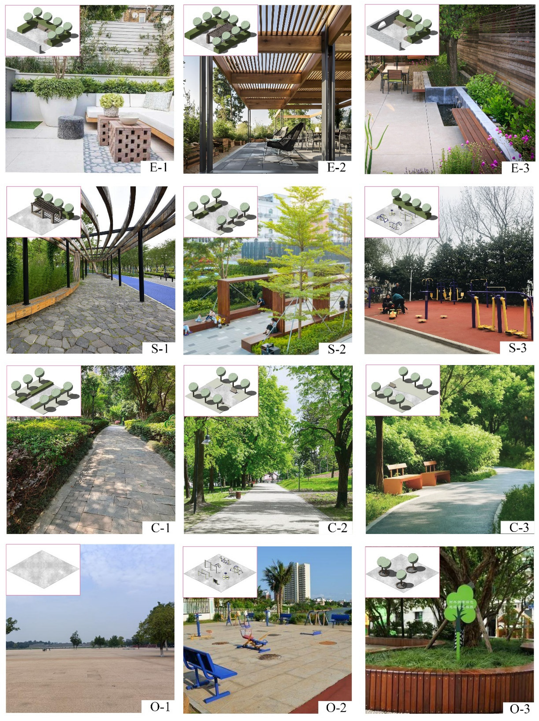
After performing a statistical analysis on the survey data, 12 types of spatial configurations were extracted and classified into the following four main categories based on previous research: closed (E-1, E-2, and E-3), semi-closed (S-1, S-2, and S-3), open (O-1, O-2, and O-3), and traffic spaces (C-1, C-2, and C-3) [72,73,74], as shown in Figure 3.
Following this, parametric modeling and constraint settings were established. Table 1 illustrates the variable system constructed through the parametric platform, which covers the following three dimensions: spatial morphology, green landscape, and site facilities. This system provides coordinated control across these elements, based on the statistical analysis of the survey data. Furthermore, the baseline model and variable range constraints were set in accordance with the guidelines in Human Dimensions of Chinese Adults [75], Technical Requirements for Sport Facilities in City Communities [76], and Code for the Design of Urban Green Space [77]. The baseline model reflects the surrounding environment and site conditions of the generated models.
Since sunlight and thermal conditions are influenced by the surrounding environment, the surrounding area was reconstructed using field survey data. A site model within a 150 m radius was established, with a focus on replicating the characteristics of high-density residential areas in Beijing, including their three-dimensional morphology and road systems. Secondary factors such as vegetation shading and artificial heat sources outside the space were neglected. As this study only focuses on the relationship between spatial morphology and environmental performance, the latent heat exchange effects and transpiration effects of plants were not considered.
The climate data layer was obtained from EnergyPlus25.1.0, using the EPW hourly meteorological file from the Beijing meteorological station (ID: 545110). These data were then corrected through Dragonfly to ensure that the simulated climate data closely aligned with real-world conditions.

3.3.2. Spatial Generation Condition Constraints and Generation Form Indicator Definitions

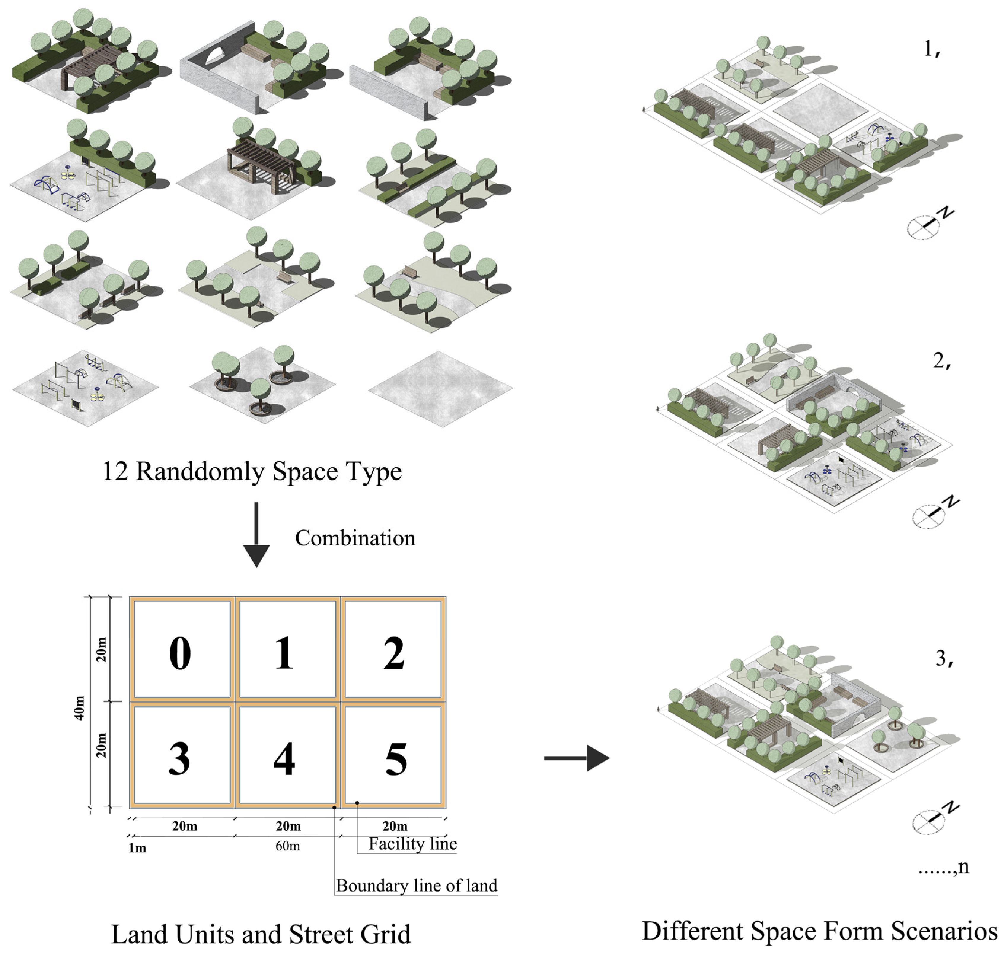
We construct a community activity space generation model using a parametric platform, as shown in Figure 4. First, 12 typical community activity space prototypes are extracted from real-world community environments and parametrically recombined to form an ideal activity space. The Grasshopper parametric platform is used to build a two-tier generation system. At the macro level, a block morphology parametric model is established based on the site environment parameters listed in Table 1. At the micro level, the standard block (60 m × 60 m) is divided into six 20 m × 20 m land units (numbered 0–5), and each unit generates an 18 m × 18 m developable space base using a double offset algorithm. The NSGA-II multi-objective optimization algorithm is then used to perform intelligent optimization of space combinations. This algorithm dynamically adjusts design variables based on performance simulation feedback to explore the optimal space configuration. It is important to note that there are 612 theoretical possibilities for the space type combinations of the six units, and the performance of each space type will undergo nonlinear changes with adjustments to the parameter thresholds in Table 1. The final generated three-dimensional model can achieve the Pareto optimal solution for space efficiency and functional adaptability through performance simulation iterations.
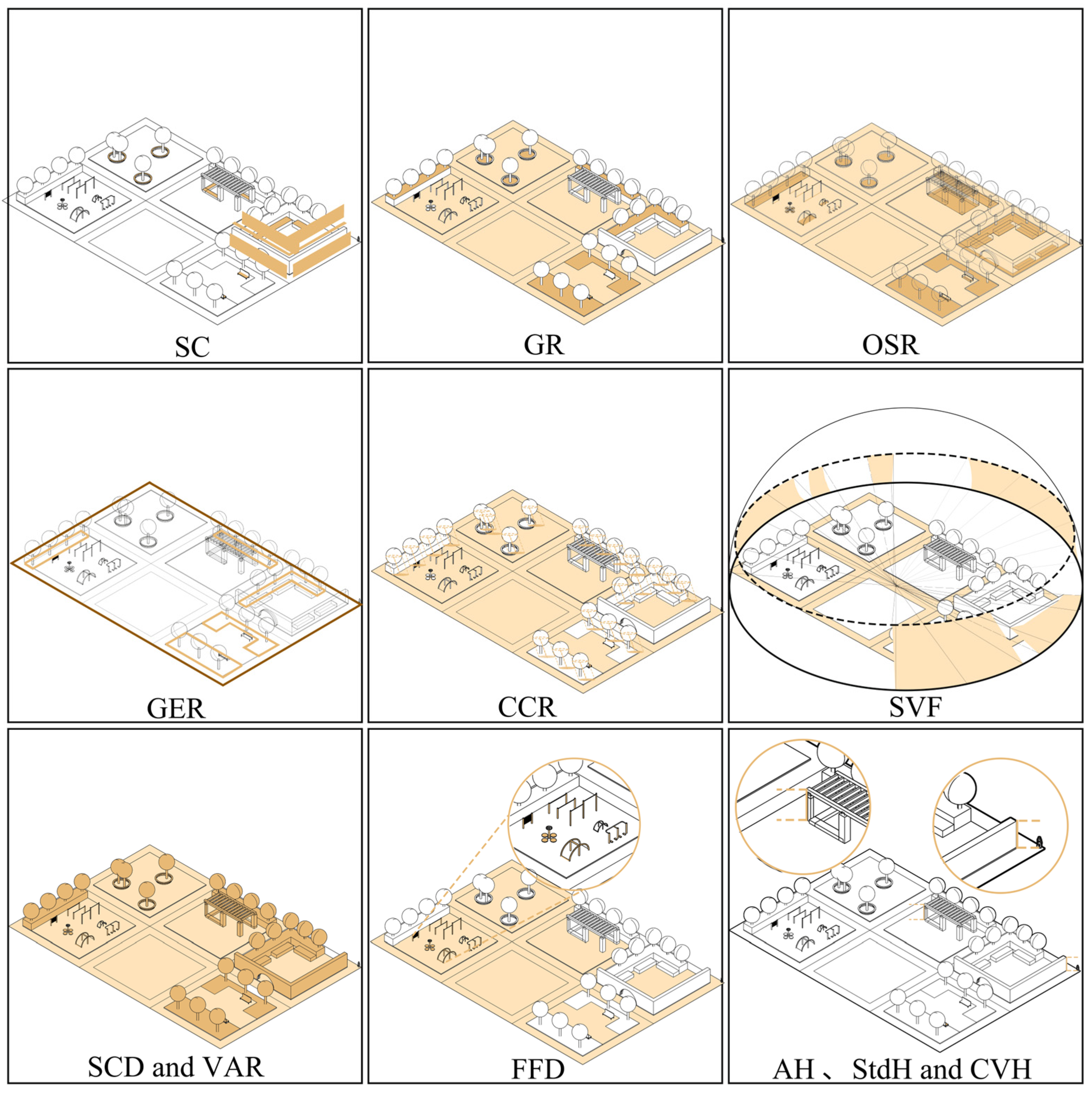
We quantify and analyze the parametric-generated activity spaces by constructing a three-dimensional morphological index system and selecting 12 shape indicators from three dimensions, as follows: space composition, green landscape, and site facilities (as shown in Table 1). The specific definitions of each indicator and their environmental relevance are given below.
(1)
Space composition indicators:
  • Average structure height (AH) and structure height standard deviation (StdH): AH represents the average height of structures within the space, reflecting the overall level of vertical variation. StdH indicates the dispersion of structure heights, reflecting the morphological diversity in the vertical dimension;
  • Spatial volume density (VAR): the ratio of structure volume to site area, used to assess the efficiency of three-dimensional space utilization;
  • Spatial crowding density (SCD): The ratio of structure volume to the product of maximum building height and site area. A higher value typically corresponds to increased shading, which may affect the site’s sunlight exposure;
  • Spatial form coefficient (SC): The ratio of the external surface area of structures (excluding ground contact surfaces) to their volume, used to reflect the complexity of the spatial form. A higher coefficient is often associated with increased interaction of environmental factors, such as wind fields and thermal radiation;
  • Open space ratio (OSR): Defined in this study as the proportion of open space without tree canopies, facilities, and structure. Higher OSR values are conducive to enhancing space ventilation and heat dissipation capabilities;
  • Coefficient of variation in spatial elevation (CVH): The ratio of the standard deviation to the mean of the structure elevations, used to quantify the richness of vertical layering in the space, which affects the formation of local microclimates;
  • Sky view factor (SVF): The proportion of visible sky from ground observation points. This parameter is significantly related to thermal comfort and has been widely used in urban thermal environment studies.
(2)
Green landscape indicators:
  • Green enclosure ratio (GER): The ratio of the length of plant–enclosed edges to the site perimeter, used to quantify the enclosing effect of vegetation, which directly affects the shading efficiency and radiation reflection;
  • Greening rate (GR): The proportion of plant-covered area to the total site area;
  • Tree canopy coverage ratio (CCR): The ratio of the total vertical projection area of all tree canopies to the site area. Given how the seasonal variation in the tree canopy size affects thermal radiation and sunlight adjustment, we set the winter canopy width to be 5–15% of the summer canopy width to explore the optimal scale of the canopy coverage.
(3)
Facility composition indicators:
  • Site facility density (FFD): The number of facilities (seats and fitness equipment) per unit area, which reflects the spatial distribution intensity of artificial elements. Through this step of quantifying spatial form, a quantitative foundation is established for the subsequent exploration of the influence mechanisms between spatial form and environmental performance. The above 12 indicators are calculated in batches using the Colibri tool in the TTtoolbox after the design schemes are generated, with the output formatted as a dataset. In the following sections of this study, this dataset is referred to as “morphological indicators.” The specific calculation formulas are shown in Table 2, and a visualization of these indicators is presented in Figure 5.
Table 2. Calculation of the morphological indicators.
DimensionIndicator SymbolFormulaNumber
AH (m) A H = i = 1 n h i × n n (1)
StdH (m) S t d H = 1 n ( h i h ¯ ) 2 (2)
CVH (m) C V H = S t d H h ¯ (3)
Spatial CompositionVAR (m) V A R = i = 1 n V o l u m e i S T (4)
SCD S C D = i = 1 n V o l u m e i H m a x S T (5)
Green CompositionSC S C = i = 1 n C i i = 1 n h i f i (6)
OSR (%) O S R = S T i = 1 n f i i = 1 n f i (7)
SVF S V F = 1 i = 1 n s i n 2 β i ( a i 360 ° ) (8)
GER (m) G E R = i = 1 n P i P s (9)
GR (m) G R = i = 1 n S G S T (10)
CCR (m) C C R = i = 1 n π r 2 S T (11)
Facility CompositionFFD F F D = i = 1 n N F S T (12)
hi denotes the height of all structures within the space;  h ¯ denotes the average height of the structures within the space; Hmax denotes the maximum height of structures within the space; volume i denotes the volume of the structures within the space; ST denotes the site area; NF denotes the number of fitness facilities; f i represents the base area of the structure; C i indicates the surface area of the structure excluding the base area; P i denotes the plant enclosure perimeter; P s represents the site perimeter; and S G signifies the total plant area within each site.

3.4. Performance Simulation and MOO

After completing the spatial morphology generation, subsequent steps involved simulating the outdoor environmental performance of the generated models. This section details the evaluation metrics and specific simulation parameters.

3.4.1. Evaluation Metrics

The Universal Thermal Climate Index (UTCI) is a comprehensive indicator used to assess human thermal comfort in outdoor environments. It integrates key meteorological parameters that affect human thermophysiological responses, including air temperature, mean radiant temperature, humidity, and wind speed [78]. Studies have shown a significant correlation between the UTCI values and elderly individuals’ thermal perception [79]. Typically, the UTCI ranges from −50 °C to +40 °C, effectively reflecting thermal comfort levels under various thermal stress conditions.
For elderly people, a UTCI range of −10 °C to +30 °C is generally considered thermally comfortable [80]. Within this range, they tend to feel relatively at ease. However, exceeding this range may cause different degrees of physiological stress. For instance, with every 10 °C decrease in the UTCI, the skin temperature of elderly individuals may drop by approximately 1.2 to 1.7 °C [81]. When the UTCI falls below −10 °C, each additional 1 °C decrease significantly increases the risk of cold-related stress responses [82]. Conversely, when the UTCI exceeds 32 °C, the risk of sudden illness in elderly individuals rises by about 10–20%; when it exceeds 38 °C, the mortality risk may increase by 25–30% [83].
Therefore, the optimal UTCI range for elderly comfort should be maintained between −10 °C and +35 °C. In this study, the UTCI was calculated at a pedestrian height of 1.5 m within urban blocks. The average UTCI value was used to reflect the overall thermal perception of elderly individuals in the study area’s outdoor environment. This index has a clear correlation with human thermal sensation [79], providing a scientific basis for thermal comfort assessments tailored to the needs of the elderly. The mathematical expression is as follows:
U T C I = T a m b + f ( T a m b , T M R T , U w i n d , P v a p o u r )
where T a m b is the ambient temperature, T M R T is the mean radiant temperature, U w i n d is the wind velocity, and P v a p o u r is the vapor pressure [84].
Sunlight hours, as a key metric for evaluating the accessibility of solar energy in outdoor spaces, specifically refer to the cumulative time during which a given area receives direct solar radiation within a defined period. In studies of urban built environments, analyzing the distribution characteristics of solar exposure can reveal the spatial restructuring effects of building layouts on light environments, providing quantitative evidence for optimizing urban morphology. Taking high-density urban areas as an example, the solar accessibility of public spaces directly affects the frequency of residents’ outdoor activities, the solar penetration rate in residential areas shows significant correlations with building energy consumption, and the solar exposure patterns in green spaces are closely tied to the carbon sequestration efficiency of ecosystems. Research demonstrates that each additional hour of effective sunshine duration in winter increases the willingness of elderly populations to engage in outdoor activities by 23% and reduces building heating demand by approximately 15% [27]. The mathematical expression for average sunlight hours is as follows:
A V . S H = T h D a y

3.4.2. Performance Simulation Parameters

Phase One: This step relies on the Urban Weather Generator (UWG) tool integrated within the Dragonfly plugin. UWG is a modeling tool specifically designed to assess urban climate impacts, and its core function is to dynamically adjust original weather data to generate microclimate data that better reflects the morphological characteristics of the study area. This enhances the accuracy of UTCI simulations and overcomes the limitations of traditional Typical Meteorological Year data at the urban scale. During this process, the EnergyPlus25.1.0 software provides standardized EPW weather data as a fundamental input for the UWG model. UWG then combines this data with three-dimensional urban morphology to dynamically adjust parameters such as urban canopy temperature and humidity, generating microclimate data with higher spatial and temporal resolution. Finally, these microclimate data are integrated into the UTCI and solar radiation calculation modules. This multi-scale fusion method has been empirically validated [85], significantly improving the accuracy and temporal continuity of thermal comfort simulations.
Phase Two: A three-dimensional numerical wind tunnel model was established based on the BlueCFD-Core fluid dynamics simulation platform. First, the refined microclimate data and wind environment parameters for the Beijing area from the first phase were imported into the wind tunnel calculation module to construct a numerical wind tunnel that conforms to the characteristics of Beijing’s urban canopy. The computational domain adopts a standard rectangular layout, as follows: the lateral and longitudinal boundary spacing was set to 5 Hspace (where Hspace is the maximum height of the generated model), and the downstream extension length was set to 10 Hspace to develop turbulence to the most realistic extent possible. Considering the characteristics of Beijing’s high-density built-up areas, the ground roughness length was set to 0.5, and the atmospheric boundary layer thickness was adjusted to 450 m. The top and lateral boundaries use symmetric boundary conditions, setting the velocity component parallel to the flow direction to zero. Specific parameters are listed in Table 3. Finally, the steady-state flow field data were output to the UTCI calculation module.
Phase Three: This phase focuses on the calculation of the mean radiant temperature (Tmrt), achieved through the Ladybug environmental analysis platform. After importing the original meteorological data from the first phase into the Tmrt calculation module, a monitoring point array with human exposure characteristics was established within the community activity space. This 4 × 8 grid monitoring system was deployed at a height of 1.5 m, focusing on analyzing the solar radiation received at each monitoring point, the dynamic changes in shading from surrounding buildings and vegetation, and the spatial geometric relationships, quantifying the thermal effects of radiation on the microclimate. All radiation calculation processes were completed using the Ladybug plugin. Additionally, since the study focuses on the correlation between spatial morphology and environmental performance, the effects of plant transpiration cooling and reflection were not considered.
Final Phase: A comprehensive UTCI evaluation was conducted, selecting typical climate periods in Beijing, including extreme heat weeks in summer and extreme cold weeks in winter, as simulation scenarios. The steady-state wind field data, dry-bulb temperature, relative humidity, and Tmrt parameters obtained from the previous steps were integrated into the UTCI calculation engine of Ladybug. Through a multi-parameter coupling algorithm, the spatial and temporal distributions of urban thermal comfort were analyzed. This integrated workflow effectively achieves the systematic conversion from basic meteorological data to thermal comfort indicators.
The simulation of sunlight hours (AV.SH) in this study was conducted using the Ladybug environmental analysis platform, and a calculation model was established by analyzing the spatiotemporal coupling relationship between the site’s geographical coordinates and the Sun’s trajectory. The specific implementation process includes the following technical points.
First, a solar trajectory algorithm model was constructed based on the site’s latitude and longitude coordinates, dynamically calculating the hourly solar altitude and azimuth angles during the simulation period. Second, the entire year was selected as the baseline period, and calibrated microclimate parameters were used to construct a two-dimensional calculation grid for the activity space. Through a sensitivity analysis, a 2 m grid resolution was determined, balancing computational efficiency and spatial resolution requirements while ensuring the reliability of radiation flux calculations. Finally, using Ladybug’s built-in radiation transfer algorithm, the cumulative sunshine hours at each grid node on a typical day were calculated, and the spatial distribution characteristics of the 4 × 8 monitoring point array were extracted. This established a quantitative evaluation system for the sunshine performance in the activity space based on the mean sunshine hours. Specific parameter settings are listed in Table 3.

3.4.3. Multi-Objective Genetic Optimization (MOGO)

Multi-objective genetic optimization (MOGO) efficiently searches the potential distribution of variable combinations to achieve the synergistic optimization of evaluation indicators. In multi-objective collaborative optimization problems, such as those involving the improvement of environmental performance with multiple interdependent indicators, the results output by the algorithm are typically presented as a nondominated solution set. The individuals within this solution set cannot be improved in one objective without causing degradation in other objectives. The resulting Pareto Front visually represents the trade-off relationships between the various objectives [86]. Its mathematical formulation is as follows:
M i n f x = f 1 x , f 2 x , f n x T S . t . g i ( x ) = ( 0 , i = 1,2 , h , x R )
Here, f i (1 ≤ i ≤ k) represents the objective functions, and g i are the constraint conditions needed to solve for the set of optimal solutions under k objective functions under h constraint conditions.
We rely on Wallcei X (a multi-objective optimization plugin based on the NSGA-II algorithm) to implement multi-objective genetic optimization. The core advantage of this plugin lies in its visual interactive interface and dynamic analysis module, which significantly enhance the interpretability of the optimization results. The NSGA-II algorithm, known for its high computational efficiency [87], ability to maintain the diversity of the Pareto solution set, and strong convergence to low-dimensional problems [62], provides theoretical support for complex multi-objective trade-off analysis. To initiate the multi-objective genetic optimization, design variables with specific ranges and intervals are defined as input data based on the parameters in Table 1. The mathematical expressions for the optimization objectives can be described as (5)–(6).
M i n f U T C I S = i = 1 n = 10 g i ( x 1 , x 2 , , x k )
M a x f U T C I W = i = 1 n = 10 g i ( x 1 , x 2 , , x k )
M a x f A V . S H = i = 1 n = 10 g i ( x 1 , x 2 , , x k )
where M a x f D F , M a x f U D I , a n d   M i n f E U I represent the three performance objectives, x 1 , x 2 , , x n represent k dimensional design variables, and the design variables are the ones shown in Table 1 of this study. g i ( x ) represents the constraint functions.
In the Wallacei platform, the optimization direction for the UTCI-S and SH (maximization) conflicts with the default minimization mode of the plugin. To resolve this, we use a reverse mapping strategy to convert both objectives negatively (i.e., the objective values are inverted), making them compatible with the algorithm’s built-in optimization logic. The specific parameter settings for the NSGA-II algorithm are shown in Table 4.

3.5. Integrated Learning Model and Spearman Correlation Analysis

After implementing the above MOO, a dataset was obtained with which to mine the mechanisms of influence in two parts. One is the morphological indicators calculated in batches, and the other is the three performance indicators simulated based on the changes in design parameters.
Based on the dataset generated from the MOO (morphological parameters and dynamic response performance indicators), we then used Spearman rank correlation analysis to analyze the nonlinear effect pathways of spatial morphology on outdoor environmental performance. This nonparametric statistical method quantifies the strength of monotonic associations between variables within the range of [−1, 1]. |ρ| → 1 represents a strong correlation, where positive values indicate synergistic effects, and negative values indicate antagonistic effects. This, ultimately, constructs a sensitivity ranking framework for key morphological factors, providing a quantitative basis for form control oriented toward light comfort.
Furthermore, given the high complexity of environmental performance, it often does not exhibit ideal linear relationships. Therefore, integrated learning algorithms, such as the RF model and the explainable machine learning algorithm SHAP, were introduced for data attribution. RF is an ensemble learning method that improves model stability and generalization by combining multiple decision trees. By aggregating the prediction results of trees trained on bootstrapped samples, it can effectively capture complex interactions between morphological features. The SHAP model, based on Shapley values, provides interpretability for each prediction value and measures the contribution of each feature to the prediction result.
Finally, based on the spatial morphological indicators extracted from both integrated learning and Spearman methods that exhibit differences, individual conditional expectation (ICE) and partial dependence plot (PDP) are plotted. The ICE plot displays a line for each instance, where the principle is to keep the values of other features constant and only change the target feature value. This helps to analyze the functional relationship between the feature variable and the model prediction result, such as whether it is linear, monotonic, or part of a more complex relationship. The PDP plot shows the marginal effect of a feature on the machine learning model’s prediction result, which can be interpreted as the averaged effect of ICE.

4. Results and Discussion

4.1. MOO Results

This study involved a total of 183 h of iteration that generated 3000 feasible solutions and 353 optimal solutions. After removing 11 duplicate solutions, 342 solutions were identified as Pareto. As shown in Figure 5, these solutions are unevenly distributed in the solution space, indicating different emphases in terms of the three optimization objectives. The four figures display the relationships between the UTCI-S, UTCI-W, and AV.SH. As shown in Figure 6b–d, the best and worst solutions for each optimization objective are selected. Figure 6a is a three-dimensional scatter plot of the three variables, where the X-axis represents the UTCI-S, ranging from approximately 30.5 °C to 33.7 °C, with lower values indicating better summer thermal comfort. The Y-axis represents the UTCI-W, ranging from −8.75 °C to 6.75 °C, with higher values indicating better winter thermal comfort. The Z-axis represents AV.SH, ranging from 4 to 8 h. The scatter plot is loosely distributed, suggesting no obvious linear correlation between these three variables. When the UTCI-S is around 32 °C, the corresponding AV.SH and UTCI-W values cover a wide range in a variety of combinations.
Figure 6c shows a certain pattern between the UTCI-S and AV.SH. As UTCI-S increases, AV.SH trends upward, indicating that longer daylight hours lead to worse summer thermal comfort (the higher the index, the worse is the thermal comfort). Similarly, Figure 6b,d show the relationships between the UTCI-S and AV.SH with the UTCI-W. The scatter plots reveal no clear linear patterns, here, suggesting no direct or simple correlation between these two variables and the UTCI-W, indicating that winter thermal comfort is not highly sensitive to daylight exposure.
In summary, although a certain linear relationship was observed between the UTCI-S and AV.SH, the relationships between the AV.SH, UTCI-S, and UTCI-W are nonlinear. This means that with respect to architectural design, solutions in the “nondominated solutions” region should be prioritized in order to balance year-round thermal comfort and daylight exposure. Additionally, the relationships between these three variables are complex, and the specific mechanisms that affect them deserve further, in-depth discussion.
A systematic comparison of the feasible and Pareto solutions in terms of thermal comfort and daylight performance was conducted using box plots (Figure 7) and reveals significant differences between the two sets of solutions in terms of environmental performance indicators. Regarding the summer outdoor thermal comfort (UTCI-S) (Figure 7a), the median of the feasible solutions is 32.5, with a range (31–33.65) approximately 21.7% broader than that of the Pareto solutions (30.8–33.38). Notably, the Pareto solutions not only reduce the upper thermal comfort threshold by 0.27 units but also narrow the interquartile range compared to the feasible solutions, indicating better thermal environment stability. The winter thermal comfort (UTCI-W) comparison (Figure 7b) shows that the feasible solutions are mainly distributed in the −8 to −7.9 range, but 12.6% of the data points are outliers below the lower threshold. In contrast, the Pareto solutions have a more concentrated distribution with fewer outliers, indicating superior stability. The AV.SH analysis (Figure 7c) shows that although the feasible solutions have a broader range (3.5–7), their coefficient of variation reaches 0.28, significantly higher than the 0.15 for the Pareto solutions. The Pareto solutions shift the effective daylight range upward (five–eight), making the median value six, with no outliers. Overall, the Pareto solutions demonstrate better central tendencies and distribution characteristics across various environmental parameters, further validating the effectiveness of the MOO algorithm in balancing environmental performance conflicts.

4.2. Algorithm Preferences and Spatial Layout Patterns

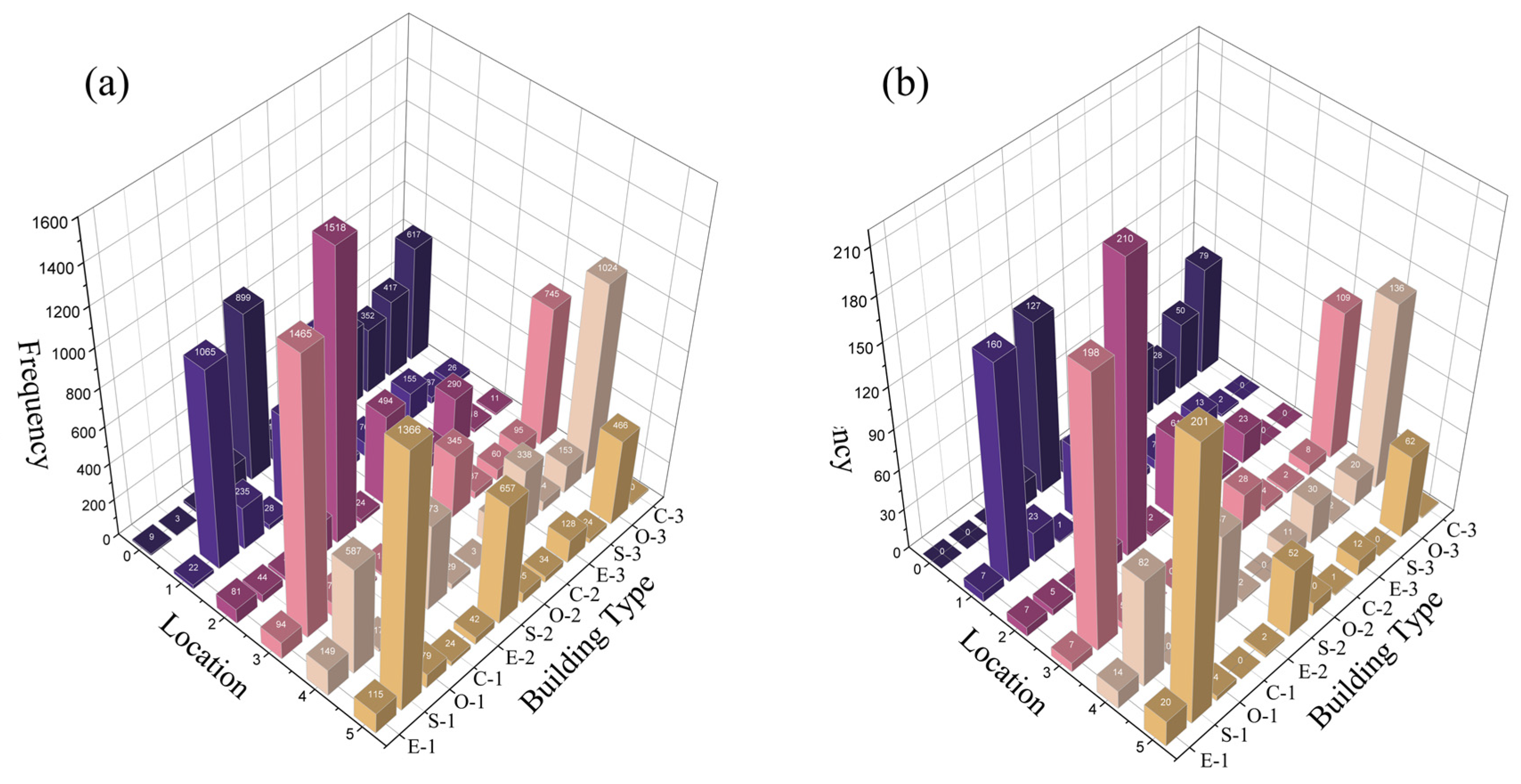
Figure 8a shows the distribution frequency of spatial types on each plot for the feasible solutions. Throughout the optimization process, the spatial types S-1, E-2, S-2, and C-3 appear most frequently, and C-1 and C-2 occur the least. Furthermore, the algorithm tends to place fully enclosed spaces (E-2) and semi-enclosed spaces (S-1 and S-3) on the northern side of the site (plots 0, 1, and 2). In contrast, the southern plots mainly consist of semi-enclosed (S-1 and S-2) and traffic spaces (C-3). The entire site shows a layout characteristic of higher ground in the north and lower ground in the south as well, with higher surrounding areas and a lower central area. The overall layout of the activity space exhibits a high–north and low–south orientation.
Figure 8b further displays the layout characteristics of the Pareto solutions. Similar to the conclusions regarding Figure 8a, S-1, E-2, S-2, and C-3 are selected most frequently by the algorithm, indicating that these types perform better. The entire site still exhibits a high–north, low–south layout, with higher surrounding areas and a lower central area. However, the proportion of S-3 decreases in the western land units, suggesting that S-3 does poorly in terms of environmental performance.

4.3. Exploring the Mechanisms by Which Spatial Morphology Impacts Environmental Performance

4.3.1. Spearman Correlation Analysis

In Section 4.2, we identified a certain relationship between the performance variables, in that summer thermal comfort is sensitive to sunlight, and winter thermal comfort is not. Based on previous studies, we hypothesize that winter thermal comfort is more sensitive to wind. To test this hypothesis, we included simulated wind speed data, labeled as WS, in the modeling process to explore the interrelationships between the variables. Specifically, the Spearman correlation coefficient was used to measure the relationships among the variables, and the statistical results are shown in Figure 9.
These results indicate that the UTCI-S has a significant positive correlation with OSR (0.57) and significant negative correlations with VAR (−0.59), SCD (−0.54), and CCR (−0.61). The UTCI-W shows significant positive correlations with SCD (0.54), CVH (0.64), and SVF (0.51), as well as a weak positive correlation with GER (0.44). It also has a significant negative correlation with wind speed (−0.91). The AV.SH shows significant positive correlations with AH (0.61) and CVH (0.53), a significant negative correlation with CCR (−0.71), and a negative correlation with StdH (−0.43). Additionally, the AV.SH has a significant positive correlation with the UTCI-S, which is similar to the results in Section 4.2.
The above suggests that the spatial morphologies in winter and summer have significant impacts on the outdoor average UTCI. In summer, the thermal environment is more sensitive to sunlight. A higher VAR (space volume density) and SCD (space congestion density) imply taller and denser buildings with higher space utilization, resulting in more continuous shadow areas and reduced solar radiation entering the space. This directly reduces solar radiation absorption on the ground and walls, thereby reducing heat accumulation in the space. Furthermore, a higher CCR (canopy coverage ratio) further reduces direct solar radiation through three-dimensional shading (e.g., colonnades and arcades), and a denser building layout may decrease air flow, preventing heat from dissipating. Moreover, a higher OSR (open space ratio), if lacking effective shading, may allow direct solar radiation to penetrate, causing surface materials to absorb and release heat, significantly raising UTCI-S. In contrast, winter thermal comfort is less sensitive to solar radiation and more significantly influenced by wind speed. Higher space utilization, taller and denser buildings, larger vegetation enclosure (GER), and richer vertical space layers (CVH) all contribute to reducing heat loss. These factors create barriers within the space, effectively reducing wind speed and, thus, decreasing convective heat loss. Additionally, lower air movement in winter helps retain heat and improve thermal comfort.
In addition, the increase in average building height (AH) expands the shadow range of tall buildings, reducing the amount of direct sunlight that enters the space. However, a higher CVH (vertical space diversity) can partially counterbalance this effect. A higher CCR (canopy coverage ratio) can block direct sunlight and reduce the duration of ground sunlight, especially when tree crowns are dense in summer. A larger building height standard deviation (StdH) may cause overlapping shadows as well, forming localized “sunlight blind spots”.

4.3.2. Random Forest and SHAP Interpretable Model Analysis

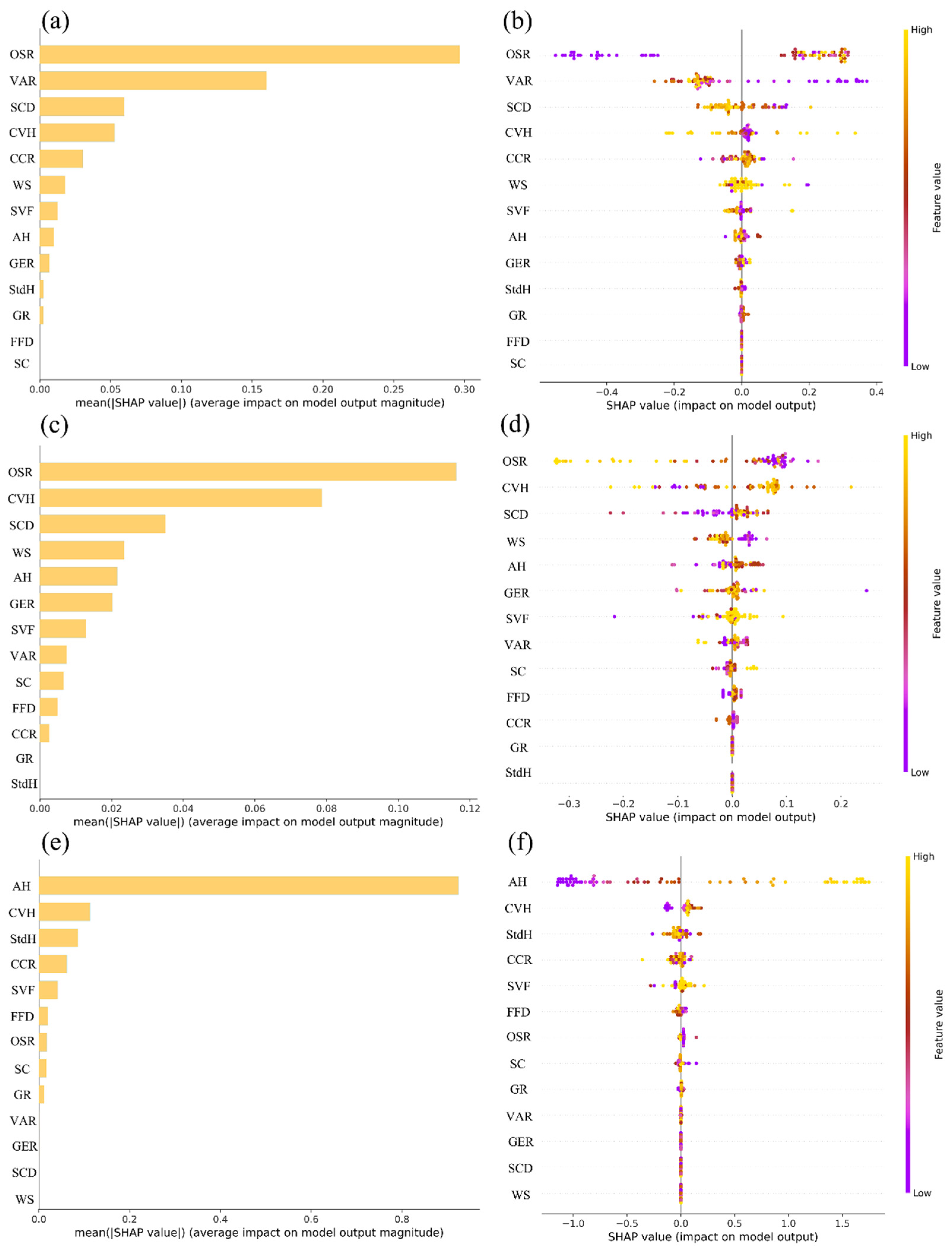
We employed Spearman correlation analysis and SHAP (Shapley additive explanations) based on the RF method to explore the impact of spatial form indicators on environmental performance (UTCI-S, UTCI-W, and AV.SH). For the best-tuned model, we performed interpretability analysis by first outputting the global feature importance ranking of the model. We then generated SHAP bar plots (Figure 10a,c,e) and summary plots (Figure 10b,d,f) for each model. In Figure 10a,c,e, the SHAP values represent the contribution of each variable to the model’s prediction. Each bar represents a variable, and the height of the bar is the absolute average of the SHAP values for all samples, indicating the magnitude of the influence of that feature on the predicted value. The bars are sorted in descending order of importance. In Figure 10b,d,f, the order of variables is consistent with that in the bar plots, where each point represents a sample. The color of the points, ranging from yellow to other colors, indicates the strength of the influence on the model. Points near SHAP = 0 are used to observe whether the variable has a positive or negative correlation with the model.
By comparing the results of the two methods, we can see that they reveal significant differences in the importance ranking of variables and the relationships between them. In Figure 10a,b, the influence of each variable on UTCI-S is ranked as OSR (+), VAR (−), SCD (−), CVH (−), and CCR (+). The OSR, VAR, and SCD are identified as important variables in both methods. However, the CCR, which shows a negative correlation (−0.61) in the Spearman correlation, is positively correlated in the RF + SHAP results. This suggests that the role of canopy coverage may exhibit nonlinear characteristics. Under certain conditions, tree shading may lower space temperatures, but in specific layouts, it may lead to heat accumulation, thus affecting the UTCI-S. CVH is not recognized in the Spearman correlation but is considered an important negative variable in the RF + SHAP results. This indicates that the Spearman method may miss certain nonlinear relationships and that XGBoost is able to capture more complex mechanisms.
Figure 10c,d show the order of the level of influence of the variables on the UTCI-W: OSR (−), CVH (−), SCD (+), WS (−), AH (+), GER (+), and SVF (+). As hypothesized, both methods emphasize the sensitivity of wind speed to the winter UTCI. The OSR and AH are captured in the ensemble learning results, and once again the Spearman analysis fails to capture this nonlinear relationship. Other variables are consistent across both methods.
In Figure 10e,f, the order of the level of influence of the variables on the AV.SH is as follows: AH (+), CVH (+), StdH (−), CCR (−), and SC (+). SVF shows a positive correlation in the machine learning method, but is not recognized in the Spearman method, suggesting that there again may be a nonlinear relationship between these variables and AV.SH. The remaining variables are consistent with the Spearman analysis. This consistent findings further support the Spearman model, but the differences in require further discussion.

4.3.3. Sensitivity Analysis and Interaction Between Variables

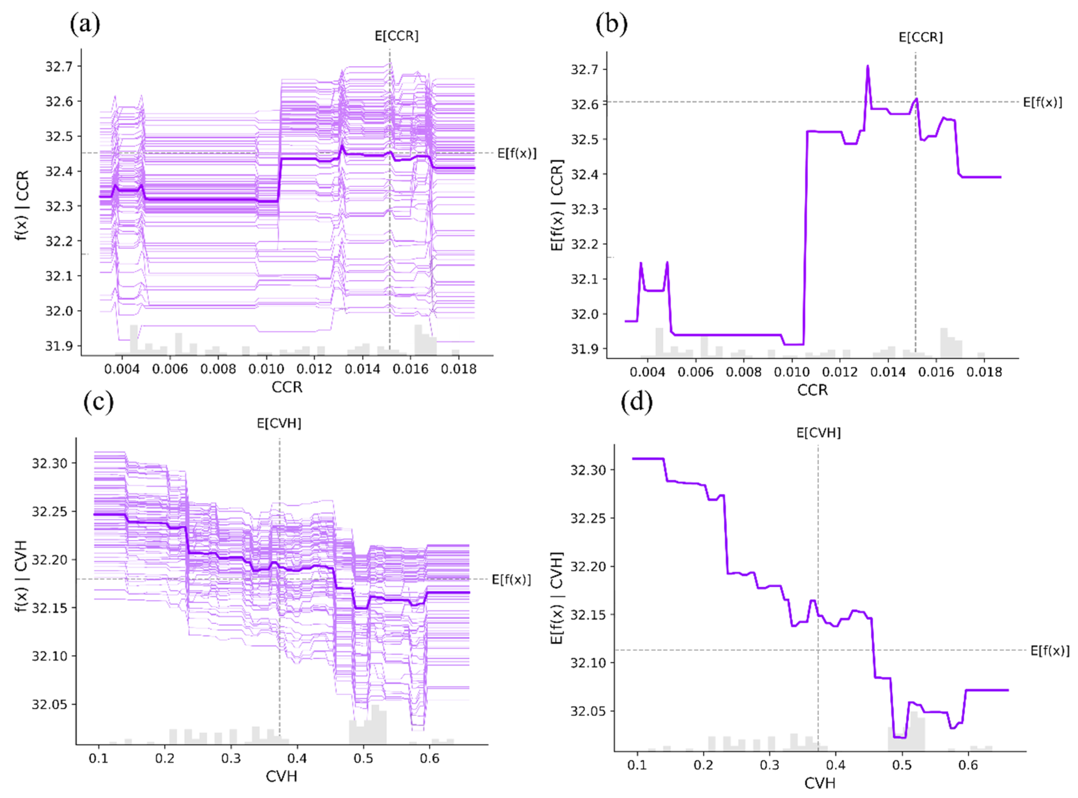
Figure 11a,c show the ICE (individual conditional expectation) plots for the CCR and CVH with respect to the UTCI-S, and Figure 11b,d present the PDP (Partial Dependence Plots) for the same variables. These results indicate that both CCR and CVH exhibit varying degrees of nonlinear relationships with the UTCI-S, accompanied by boundary effects. Specifically, for the CCR, the ICE plot shows that the UTCI-S values are not sensitive to changes in the CCR across all samples, with only a weak positive correlation. Additionally, the PDP plot reveals that for the average sample, the impact of the CCR on the UTCI-S is unstable when the CCR is less than 0.005. When the CCR ranges from 0.005 to 0.013, however, a positive correlation with the UTCI-S is observed, though values between 0.013 and 0.0165 exhibit a negative correlation. At the CCR = 0.0165, a critical point is reached. The discovery of this critical value holds practical significance for architects, as follows: when 0.013 < CCR < 0.0165, increasing the CCR can effectively reduce the summer UTCI.
For CVH, the entire sample shows a negative correlation with the UTCI-S. For the mean sample, this negative correlation persists, but two critical points appear when 0.6 > CVH > 0.15, where it continues to correlate negatively with the UTCI-S, even as the rest of the range remains unchanged. This suggests that when the CVH < 0.6, increasing vertical variation in space can effectively reduce thermal discomfort.
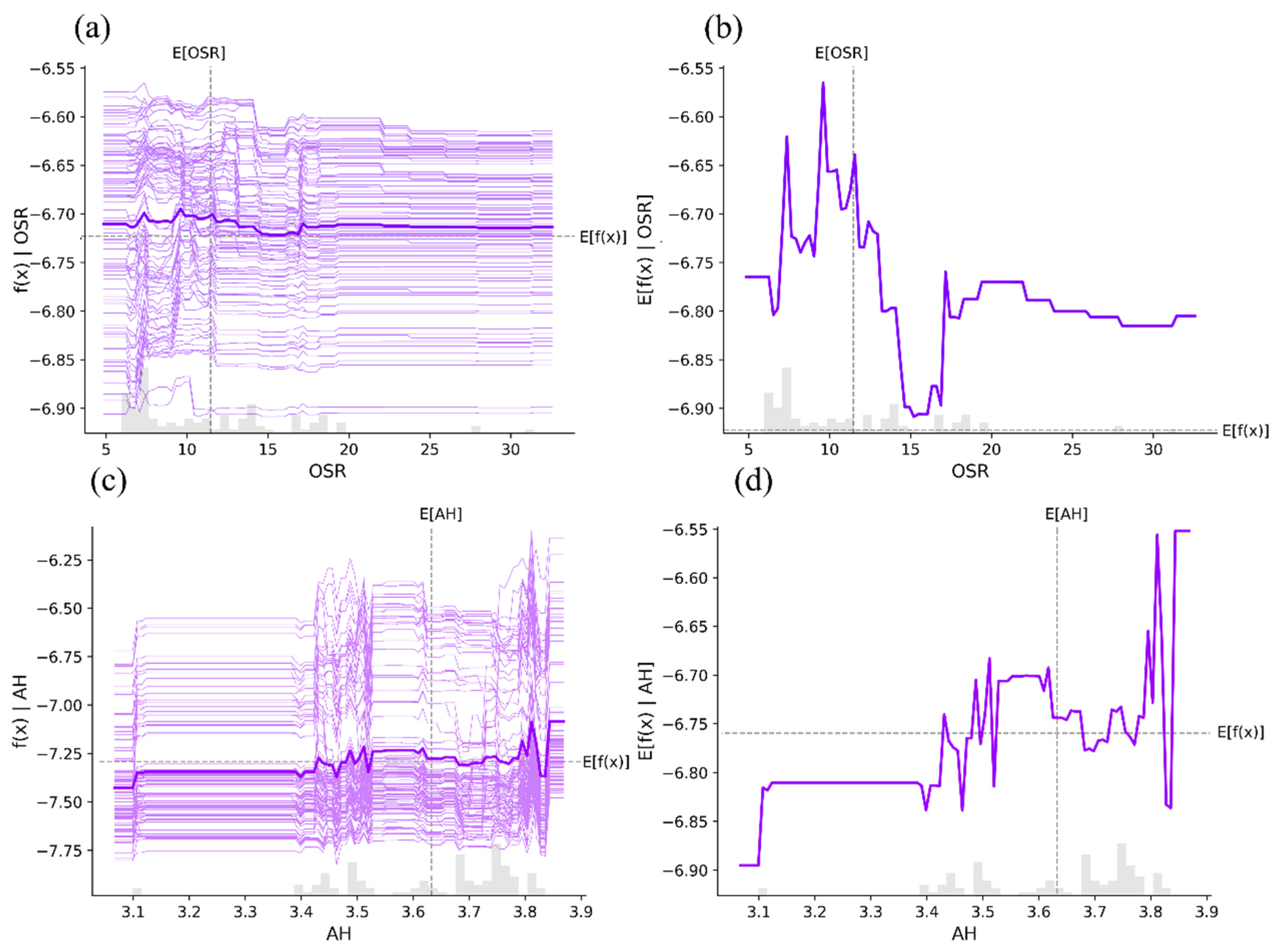
The relationship between the OSR and AH with respect to the UTCI-W is analyzed in Figure 12. These results show that the OSR and AH exhibit varying degrees of nonlinear correlations with the UTCI-W, accompanied by boundary effects. Specifically, for the OSR, Figure 12a reveals that the UTCI-W values across all samples were not sensitive to changes in the OSR, and Figure 11b indicates that for the average sample, when the OSR was less than 12, its impact on the UTCI-W was unstable. However, when the OSR was between 11 and 15, it shows a negative correlation with the UTCI-W, though between 15 and 17 a positive correlation is observed. After the OSR exceeded 20, the effect stabilized. This suggests that in spatial design, when 15 > OSR > 10, increasing the OSR can improve winter thermal comfort, whereas the OSR values greater than 15 inhibit winter thermal comfort.
For AH, Figure 12c shows a weak positive correlation between the AH and UTCI-W across all samples. Figure 12d further reveals that for the average sample, a positive correlation was observed between the AH values of 3.1 to 3.6 and 3.7 to 3.8, but a negative correlation was found between 3.6 and 3.7. When the AH exceeded 3.85, the UTCI-W no longer changed, however. This implies that in winter, increasing the height of buildings in the active space can effectively block winter winds, but when AH exceeds 3.9, this effect becomes negligible.
Figure 13 shows the relationship between the SCF and AV.SH. There is a noticeable nonlinear correlation between the SVF and UTCI-W. In Figure 13a, across all samples, the AV.SH shows a weak positive correlation with SVF. Figure 13b further reveals that for the average sample, when SVF was less than 0.6, there was a significant positive correlation with the AV.SH. However, when the SVF exceeded 0.6, after slight fluctuations the correlation stabilized, indicating that the AV.SH no longer changed with variations in the SVF. This suggests that in spatial design, simply increasing the SVF does not necessarily improve daylight within the space.

5. Conclusions

This study focused on optimizing the environmental comfort of outdoor public activity spaces in communities in Beijing. Data on the site and spatial morphology of 63 community activity spaces in Beijing were collected, and 12 spatial types were abstracted through statistical analysis. The design variables and constraints for the study were then determined, and parametric tools were used to generate ideal community spaces.
The NSGA-II multi-objective optimization algorithm was applied to minimize summer outdoor thermal comfort, maximize winter outdoor thermal comfort, and maximize the annual average daylight hours, which resulted in 342 Pareto optimal solutions. The linear relationship between spatial morphology and environmental performance was first explored using the Spearman method. Subsequently, a nonlinear relationship and boundary effects were revealed through the application of ensemble learning combined with the interpretable machine learning model SHAP. The results of these two approaches are complementary and mutually reinforcing. Based on the comparative results, morphological indicators showing significant differences between the two methods were selected for data attribution and sensitivity analysis. By isolating individual data points, the underlying causes of these differences were examined, and threshold effects in the relationship between spatial morphology and environmental performance were identified. The core findings of this chapter offer valuable practical guidance for architects in designing outdoor public spaces that meet the comfort needs of elderly populations.
(1)
Linear and Nonlinear Relationships:
  • UTCI-S is linearly related to OSR (+), VAR (−), SCD (−) and nonlinearly related to CVH (−), CCR (+);
  • UTCI-W is linearly related to CVH (−), SCD (+), WS (−), GER (+), SVF (+), and nonlinearly related to OSR (−), AH (+);
  • AV.SH is linearly related to AH (+), CVH (+), StdH (−), CCR (−), and SVF (+).
(2)
Boundary Effects:
The CCR and CVH exhibit significant boundary effects on the UTCI-S, AH on the UTCI-W, and SVF on the AV.SH. A critical threshold was observed at a CCR = 0.0165, which holds practical value for architectural design. When 0.013 < CCR < 0.0165, increasing the CCR can effectively reduce the summer UTCI. Similarly, when 0.15 < CVH < 0.6, enhancing vertical height variation within the space can help alleviate thermal discomfort in summer. For the OSR, values between 11 and 15 show a negative correlation with the UTCI-W; between 15 and 17, the correlation becomes positive; and beyond 20, it tends to stabilize. In addition, the UTCI-W remains unchanged when the AH > 3.85 m, suggesting that excessively increasing building height to block winter wind may become ineffective beyond this point.
(3)
Sensitivity to Light and Wind:
UTCI-S is more sensitive to light, and UTCI-W is more sensitive to wind.
(4)
Spatial Types and Layout:
There is a pattern for spatial types and layouts. Enclosed spaces (E-2) and semi-enclosed spaces (S-1, S-3) are optimally placed on the northern side of the site, and southern plots are primarily used for semi-enclosed (S-1, S-2) and traffic spaces (C-3), where their overall spatial performance is optimal.
Based on these findings, we propose the following design strategies.
(1)
Space Layout:
The northern side of community activity spaces should be arranged with enclosed or semi-enclosed spaces to reduce the impact of north winds on activity areas and to improve overall microclimate comfort. The southern side should comprise semi-enclosed and traffic spaces to enhance sunlight utilization.
(2)
Open Space Ratio:
The open space ratio should be controlled between 10–15% to balance winter and summer thermal comfort.
(3)
Tree and Shrub Coverage:
The tree and shrub coverage ratio should be controlled between 0.013 and 0.0165.
(4)
Vertical Space Variation:
The vertical space variation should be appropriately increased between 0.15 and 0.6.
(5)
Building Height:
The average building height (AH) should be between 3.1 and 3.6 m or 3.7 and 3.8 m.
Our research reveals the mechanisms by which different spatial morphological features affect environmental performance and provides scientific evidence that can guide the design of spatial forms. However, the study does have limitations. First, we only selected spaces in cold regions as samples, so the generalizability of the results needs to be further validated in different cities and climates. Second, although the study considered the geometric morphological characteristics of plants, it did not account for factors such as plant transpiration cooling and latent heat exchange.

Author Contributions

Fang Wen and Lu Zhang: Conceptualization, methodology, writing—review and editing, data curation, formal analysis, investigation, software, visualization, and writing—original draft; Ling Jiang and Rui Tang: methodology, writing—review and editing, data curation, formal analysis, investigation, software, visualization, and writing—original draft; Fang Wen and Bo Zhang: funding acquisition, project administration, supervision, and writing—review and editing. All authors have read and agreed to the published version of the manuscript.

Funding

The Youth Project of Humanities and Social Sciences Fund of the Ministry of Education (grant no. 21YJCZH174).

Informed Consent Statement

This study did not involve humans.

Data Availability Statement

Data will be made available upon request.

Acknowledgments

The authors thank to the student Wenqi Sun for his contribution to the literature collection of this article.

Conflicts of Interest

The authors declare no conflicts of interest.

Abbreviations

UTCIUniversal Thermal Climate Index
UTCI-SUniversal Thermal Climate Index—Summer
UTCI-WUniversal Thermal Climate Index—Winter
AV.SHThe Simulation Of Sunlight Hours
OSROpen Space Ratio
SCDSpace Congestion Density
CVHCanopy Coverage
WSWind Speed
SVFSky View Factor
WHOThe World Health Organization
TMRTTemperature
OHCAOut-Of-Hospital Cardiac Arrest
CFDComputational Fluid Dynamics
PETPhysiological Equivalent Temperature
SVRSupport Vector Regression
MOOMulti-Objective Optimization
GAsGenetic Algorithms
PSOParticle Swarm Optimization
NSPSONondominated Sorting Particle Swarm Optimization
MLRMultiple Linear Regression
ANNArtificial Neural Networks
RFRandom Forests
ICEIndividual Conditional Expectation
PDPPartial Dependence Plots
SHAPShapley Additive Explanations
AHAverage Building Height
STDHStandard Deviation
VARSpace Volume Density
SCSpatial Form Coefficient
GERGreen Enclosure Degree
GRGreening Rate
CCRCanopy Coverage Ratio
FFDSite Facility Density
TMYTypical Meteorological Year
UWGUrban Weather Generator
MOGOMulti-Objective Genetic Optimization

References

  1. National Bureau of Statistics. China Statistical Yearbook; China Statistics Press: Beijing, China, 2023.
  2. Sun, S.; Yu, Z.; An, S. Patterns of Physical and Mental Co-Occurring Developmental Health among Chinese Elderly: A Multidimensional Growth Mixture Model Analysis. SSM—Popul. Health 2024, 25, 101584. [Google Scholar] [CrossRef] [PubMed]
  3. Zhang, Y.; Kuang, J.; Xin, Z.; Fang, J.; Song, R.; Yang, Y.; Song, P.; Wang, Y.; Wang, J. Loneliness, Social Isolation, Depression and Anxiety among the Elderly in Shanghai: Findings from a Longitudinal Study. Arch. Gerontol. Geriatr. 2023, 110, 104980. [Google Scholar] [CrossRef] [PubMed]
  4. Ding, Z.; Zhang, X.; Yi, C. Study on Behavior Characteristics, Support and Influencing Factors of Physical Exercise of the Elderly in Urban China. Lanzhou Acad. J. 2020, 6, 174–187. [Google Scholar] [CrossRef]
  5. Yuan, K.S.; Wu, T.J. Environmental Stressors and Well-Being on Middle-Aged and Elderly People: The Mediating Role of Outdoor Leisure Behaviour and Place Attachment. Environ. Sci. Pollut. Res. 2021. [CrossRef]
  6. Petersen, J.; Austin, D.; Kaye, J.A.; Pavel, M.; Hayes, T.L. Unobtrusive In-Home Detection of Time Spent out-of-Home with Applications to Loneliness and Physical Activity. IEEE J. Biomed. Health Inform. 2014, 18, 1590–1596. [Google Scholar] [CrossRef]
  7. Cedervall, Y.; Torres, S.; Åberg, A.C. Maintaining Well-Being and Selfhood through Physical Activity: Experiences of People with Mild Alzheimer’s Disease. Aging Ment. Health 2015, 19, 679–688. [Google Scholar] [CrossRef]
  8. Zhu, D.; Liu, G.; Lv, Z.; Wen, S.; Bi, S.; Wang, W. Inverse Associations of Outdoor Activity and Vitamin D Intake with the Risk of Parkinson’s Disease. J. Zhejiang Univ. Sci. B 2014, 15, 923–927. [Google Scholar] [CrossRef]
  9. Suzuki, T.; Murase, S. Influence of Outdoor Activity and Indoor Activity on Cognition Decline: Use of an Infrared Sensor to Measure Activity. Telemed. E Health 2010, 16, 686–690. [Google Scholar] [CrossRef]
  10. Pleson, E.; Nieuwendyk, L.M.; Lee, K.K.; Chaddah, A.; Nykiforuk, C.I.J.; Schopflocher, D. Understanding Older Adults’ Usage of Community Green Spaces in Taipei, Taiwan. Int. J. Environ. Res. Public Health 2014, 11, 1444. [Google Scholar] [CrossRef]
  11. Chiesura, A. The Role of Urban Parks for the Sustainable City. Landscape Urban Plann. 2004, 68, 129–138. [Google Scholar] [CrossRef]
  12. Tang, T.; Zhou, X.; Zhang, Y.; Feng, X.; Liu, W.; Fang, Z.; Zheng, Z. Investigation into the Thermal Comfort and Physiological Adaptability of Outdoor Physical Training in College Students. Sci. Total Environ. 2022, 839, 155979. [Google Scholar] [CrossRef] [PubMed]
  13. Lau, K.K.-L.; Choi, C.Y. The Influence of Perceived Aesthetic and Acoustic Quality on Outdoor Thermal Comfort in Urban Environment. Build. Environ. 2021, 206, 108333. [Google Scholar] [CrossRef]
  14. Yin, Y.; Zhang, D.; Zhen, M.; Jing, W.; Luo, W.; Feng, W. Combined Effects of the Thermal-Acoustic Environment on Subjective Evaluations in Outdoor Public Spaces. Sustain. Cities Soc. 2022, 77, 103522. [Google Scholar] [CrossRef]
  15. World Health Organization. World Report on Ageing and Health; World Health Organization: Geneva, Switzerland, 2015; ISBN 978-92-4-156504-2. [Google Scholar]
  16. Ou, Y.; Wang, F.; Zhao, J.; Deng, Q. Risk of Heatstroke in Healthy Elderly during Heatwaves: A Thermoregulatory Modeling Study. Build. Environ. 2023, 237, 110324. [Google Scholar] [CrossRef]
  17. Wang, J.; Li, Q.; Zhu, G.; Kong, W.; Peng, H.; Wei, M. Recognition and Prediction of Elderly Thermal Sensation Based on Outdoor Facial Skin Temperature. Build. Environ. 2024, 253, 111326. [Google Scholar] [CrossRef]
  18. Ji, Y.; Feng, X.; Zhao, H.; Xu, X. Study on the Elderly’s Perception of Microclimate and Activity Time in Residential Communities. Build. Environ. 2024, 266, 112125. [Google Scholar] [CrossRef]
  19. Ma, X.; Song, L.; Hong, B.; Li, Y.; Li, Y. Relationships between EEG and Thermal Comfort of Elderly Adults in Outdoor Open Spaces. Build. Environ. 2023, 235, 110212. [Google Scholar] [CrossRef]
  20. Li, J.; Wang, J.; Niu, J. Elderly Residents’ Uses of Fragmented Outdoor Spaces in Public Housing Estates in Hong Kong—Decoding Causality and Heat-Risk Exposure. Build. Environ. 2023, 245, 110912. [Google Scholar] [CrossRef]
  21. Xu, F.; Gao, Z.; Zhang, J.; Hu, Y.; Ding, W. Influence of Typical Street-Side Public Building Morphologies on the Ventilation Performance of Streets and Squares. Build. Environ. 2022, 221, 109331. [Google Scholar] [CrossRef]
  22. Fei, F.; Wang, Y.; Wang, L.; Fukuda, H.; Yao, W. Influence of Greenery Configuration on Summer Thermal Environment of Outdoor Recreational Space in Elderly Care Centers. Build. Environ. 2023, 245, 110857. [Google Scholar] [CrossRef]
  23. Jiao, Y.; Yu, Y.; Yu, H.; Wang, F. The Impact of Thermal Environment of Transition Spaces in Elderly-Care Buildings on Thermal Adaptation and Thermal Behavior of the Elderly. Build. Environ. 2023, 228, 109871. [Google Scholar] [CrossRef]
  24. Wang, B.; Jiang, X.; Han, B.; Zhao, H. An Investigation of Outdoor Thermal Comfort Assessment for Elderly Individuals in a Field Study in Northeastern China. Buildings 2023, 13, 2458. [Google Scholar] [CrossRef]
  25. Wang, J.; Li, J.; Niu, J. Assessment of Multi-Factor Influences on Elderly Usage Patterns and Heat-Stress Exposure in Neighbourhood Public Outdoor Spaces. Build. Environ. 2025, 268, 112340. [Google Scholar] [CrossRef]
  26. Qiu, H.; Sun, S.; Tang, R.; Chan, K.-P.; Tian, L. Pneumonia Hospitalization Risk in the Elderly Attributable to Cold and Hot Temperatures in Hong Kong, China. Am. J. Epidemiol. 2016, 184, 570–578. [Google Scholar] [CrossRef]
  27. Low, C.T.; Lai, P.C.; Yeung, P.S.; Siu, A.Y.; Leung, K.T.; Wong, P.P.Y. Temperature and Age–Gender Effects on out-of-Hospital Cardiac Arrest Cases. Hong Kong J. Emerg. Med. 2018, 25, 102490791775130. [Google Scholar] [CrossRef]
  28. Zhao, Y.; Huang, Z.; Wang, S.; Hu, J.; Xiao, J.; Li, X.; Liu, T.; Zeng, W.; Guo, L.; Du, Q.; et al. Morbidity Burden of Respiratory Diseases Attributable to Ambient Temperature: A Case Study in a Subtropical City in China. Environ. Health 2019, 18, 89. [Google Scholar] [CrossRef]
  29. Hussainzad, E.A.; Gou, Z. Exploring the Impact of Demographic, Architectural, and Well-Being Factors on Health Outcomes in Informal Settlements: The Role of Daylight, Window Depth, and Building Orientation. Wellbeing Space Soc. 2025, 8, 100242. [Google Scholar] [CrossRef]
  30. Karaman Madan, Ö.; Chamilothori, K.; van Duijnhoven, J.; Aarts, M.P.J.; de Kort, Y.A.W. Restorative Effects of Daylight in Indoor Environments—A Systematic Literature Review. J. Environ. Psychol. 2024, 97, 102323. [Google Scholar] [CrossRef]
  31. Kööts, L.; Realo, A.; Allik, J. The Influence of the Weather on Affective Experience. J. Individ. Differ. 2011, 32, 74–84. [Google Scholar] [CrossRef]
  32. Webb, A.; Pilbeam, C.; Hanafin, N.; Holick, M. An Evaluation of the Relative Contributions of Exposure to Sunlight and of Diet to the Circulating Concentrations of 25-Hydroxyvitamin D in an Elderly Nursing Home Population in Boston. Am. J. Clin. Nutr. 1990, 51, 1075–1081. [Google Scholar] [CrossRef]
  33. Song, Y.; Duan, Q.; Feng, Y.; Zhang, E.; Wang, J.; Niu, S. Solar Infrared Radiation towards Building Energy Efficiency: Measurement, Data, and Modeling. Environ. Rev. 2020, 28, 457–465. [Google Scholar] [CrossRef]
  34. Wang, S.; Yi, Y.K.; Liu, N. Multi-Objective Optimization (MOO) for High-Rise Residential Buildings’ Layout Centered on Daylight, Visual, and Outdoor Thermal Metrics in China. Build. Environ. 2021, 205, 108263. [Google Scholar] [CrossRef]
  35. Fan, Z.; Liu, M.; Tang, S.; Zong, X. Multi-Objective Optimization for Gymnasium Layout in Early Design Stage: Based on Genetic Algorithm and Neural Network. Build. Environ. 2024, 258, 111577. [Google Scholar] [CrossRef]
  36. Li, J.; Niu, J.; Huang, T.; Mak, C.M. Dynamic Effects of Frequent Step Changes in Outdoor Microclimate Environments on Thermal Sensation and Dissatisfaction of Pedestrian during Summer. Sustain. Cities Soc. 2022, 79, 103670. [Google Scholar] [CrossRef]
  37. Qaoud, R.; Adel, B.; Sayad, B.; Alkama, D.; Attia, S. Assessing the Influence of Neighborhood Urban Form on Outdoor Thermal Conditions in the Hot Dry City of Biskra, Algeria. Ain Shams Eng. J. 2023, 14, 102525. [Google Scholar] [CrossRef]
  38. Suga, K.; Kato, S.; Hiyama, K. Structural Analysis of Pareto-Optimal Solution Sets for Multi-Objective Optimization: An Application to Outer Window Design Problems Using Multiple Objective Genetic Algorithms. Build. Environ. 2010, 45, 1144–1152. [Google Scholar] [CrossRef]
  39. Li, N.; Cheung, S.C.P.; Li, X.; Tu, J. Multi-Objective Optimization of HVAC System Using NSPSO and Kriging Algorithms—A Case Study. Build. Simul. 2017, 10, 769–781. [Google Scholar] [CrossRef]
  40. Zhan, X.; Zhang, W.; Chen, R.; Bai, Y.; Wang, J.; Deng, G. Non-Dominated Sorting Genetic Algorithm-II: A Multi-Objective Optimization Method for Building Renovations with Half-Life Cycle and Economic Costs. Build. Environ. 2025, 267, 112155. [Google Scholar] [CrossRef]
  41. Wang, Y.; Li, J.; Liu, W.; Dong, J.; Liu, J. Integrating NSGA-II and CFD for Enhanced Urban Airflow Prediction: Recalibration of Closure Coefficients for a Nonlinear Eddy Viscosity Model. Build. Environ. 2024, 259, 111627. [Google Scholar] [CrossRef]
  42. Wei, H.; Jiao, Y.; Wang, Z.; Wang, W.; Zhang, T. Optimal Retrofitting Scenarios of Multi-Objective Energy-Efficient Historic Building under Different National Goals Integrating Energy Simulation, Reduced Order Modelling and NSGA-II Algorithm. Build. Simul. 2024, 17, 933–954. [Google Scholar] [CrossRef]
  43. Fesanghary, M.; Asadi, S.; Geem, Z.W. Design of Low-Emission and Energy-Efficient Residential Buildings Using a Multi-Objective Optimization Algorithm. Build. Environ. 2012, 49, 245–250. [Google Scholar] [CrossRef]
  44. Lin, B.; Chen, H.; Liu, Y.; He, Q.; Li, Z. A Preference-Based Multi-Objective Building Performance Optimization Method for Early Design Stage. Build. Simul. 2021, 14, 477–494. [Google Scholar] [CrossRef]
  45. Wani, M.; Swain, A.; Ukil, A.; Ploder, M.; Koole, R. Optimizing the Overall Performance of Forced Extraction Systems: A Multi-Objective Framework. Build. Environ. 2022, 221, 109214. [Google Scholar] [CrossRef]
  46. Wu, C.; Pan, H.; Luo, Z.; Liu, C.; Huang, H. Multi-Objective Optimization of Residential Building Energy Consumption, Daylighting, and Thermal Comfort Based on BO-XGBoost-NSGA-II. Build. Environ. 2024, 254, 111386. [Google Scholar] [CrossRef]
  47. Li, X.; Lu, W.; Peng, Z.; Zhang, Y.; Huang, J. Generative Design of Walkable Urban Cool Spots Using a Novel Heuristic GAN×GAN Approach. Build. Environ. 2024, 266, 112027. [Google Scholar] [CrossRef]
  48. Reitberger, R.; Palm, N.; Palm, H.; Lang, W. Urban Systems Exploration: A Generic Process for Multi-Objective Urban Planning to Support Decision Making in Early Design Phases. Build. Environ. 2024, 254, 111360. [Google Scholar] [CrossRef]
  49. Chipman, J.S. Linear Restrictions, Rank Reduction, and Biased Estimation in Linear Regression. Linear Algebra Appl. 1999, 289, 55–74. [Google Scholar] [CrossRef]
  50. Yamamoto, Y.; Perron, P. Estimating and Testing Multiple Structural Changes in Linear Models Using Band Spectral Regressions. Econom. J. 2013, 16, 400–429. [Google Scholar] [CrossRef]
  51. Noi, P.; Degener, J.; Kappas, M. Comparison of Multiple Linear Regression, Cubist Regression, and Random Forest Algorithms to Estimate Daily Air Surface Temperature from Dynamic Combinations of MODIS LST Data. Remote Sens. 2017, 9, 398. [Google Scholar] [CrossRef]
  52. Azriel, D.; Brown, L.D.; Sklar, M.; Berk, R.; Buja, A.; Zhao, L. Semi-Supervised Linear Regression. J. Am. Stat. Assoc. 2022, 117, 2238–2251. [Google Scholar] [CrossRef]
  53. Wu, S.; Sun, J.-Q. Multi-Stage Regression Linear Parametric Models of Room Temperature in Office Buildings. Build. Environ. 2012, 56, 69–77. [Google Scholar] [CrossRef]
  54. Wang, B.; Cot, L.D.; Adolphe, L.; Geoffroy, S.; Sun, S. Cross Indicator Analysis between Wind Energy Potential and Urban Morphology. Renew. Energy 2017, 113, 989–1006. [Google Scholar] [CrossRef]
  55. Egrioglu, E.; Bas, E. A New Deep Neural Network for Forecasting: Deep Dendritic Artificial Neural Network. Artif. Intell. Rev. 2024, 57, 171. [Google Scholar] [CrossRef]
  56. Huang, W.; Liu, H.; Zhang, Y.; Mi, R.; Tong, C.; Xiao, W.; Shuai, B. Railway Dangerous Goods Transportation System Risk Identification: Comparisons among SVM, PSO-SVM, GA-SVM and GS-SVM. Appl. Soft Comput. 2021, 109, 107541. [Google Scholar] [CrossRef]
  57. Sun, J.; Zhong, G.; Huang, K.; Dong, J. Banzhaf Random Forests: Cooperative Game Theory Based Random Forests with Consistency. Neural Netw. 2018, 106, 20–29. [Google Scholar] [CrossRef]
  58. Chen, T.; Guestrin, C. XGBoost: A Scalable Tree Boosting System. In Proceedings of the 22nd ACM SIGKDD International Conference on Knowledge Discovery and Data Mining, San Francisco, CA, USA, 13–17 August 2016; pp. 785–794. [Google Scholar]
  59. Moosavi, N.; Bagheri, M.; Nabi-Bidhendi, M.; Heidari, R. Porosity Prediction Using Fuzzy SVR and FCM SVR from Well Logs of an Oil Field in South of Iran. Acta Geophys. 2022, 71, 769–782. [Google Scholar] [CrossRef]
  60. Sun, Y.; Ding, S.; Zhang, Z.; Jia, W. An Improved Grid Search Algorithm to Optimize SVR for Prediction. Soft Comput. 2021, 25, 5633–5644. [Google Scholar] [CrossRef]
  61. Ayerdi, B.; Graña, M. Hybrid Extreme Rotation Forest. Neural Netw. 2014, 52, 33–42. [Google Scholar] [CrossRef]
  62. Nohara, Y.; Matsumoto, K.; Soejima, H.; Nakashima, N. Explanation of Machine Learning Models Using Improved Shapley Additive Explanation. In Proceedings of the 10th ACM International Conference on Bioinformatics, Computational Biology and Health Informatics, Niagara Falls, NY, USA, 7–10 September 2019; p. 546. [Google Scholar] [CrossRef]
  63. Mandal, B.; Roy, P.K. Multi-Objective Optimal Power Flow Using Grasshopper Optimization Algorithm. Optim. Control. Appl. Methods 2024, 45, 623–645. [Google Scholar] [CrossRef]
  64. Ladybug Tools|Dragonfly, (n.d.). Available online: https://www.ladybug.tools/dragonfly.html (accessed on 16 March 2025).
  65. Ladybug Tools|Ladybug, (n.d.). Available online: https://www.ladybug.tools/ladybug.html (accessed on 16 March 2025).
  66. Ladybug Tools|Butterfly, (n.d.). Available online: https://www.ladybug.tools/butterfly.html (accessed on 16 March 2025).
  67. BlueCFD. (n.d.). BlueCFD-Core. Available online: https://bluecfd.github.io/Core/ (accessed on 16 March 2025).
  68. Evolutionary Engine for Grasshopper3D, Wallacei (n.d.). Available online: https://www.wallacei.com (accessed on 16 March 2025).
  69. TT Toolbox, Food4Rhino (2013). Available online: https://www.food4rhino.com/en/app/tt-toolbox (accessed on 16 March 2025).
  70. Python Software Foundation. (n.d.). Python Official Website. Available online: https://www.python.org/ (accessed on 16 March 2025).
  71. Report on the Development of the Elderly Career in Beijing, 2023. National Bureau of Statistics of China. Available online: https://www.gov.cn/lianbo/difang/202410/content_6979496.htm (accessed on 16 March 2025). (In Chinese)
  72. Xu, F.; Li, C.; Tang, H. Influence Analysis of Space Configuration on Cooling Load of a Large Semi-Closed Atrium in Hot and Humid Region. Build. Environ. 2022, 225, 109670. [Google Scholar] [CrossRef]
  73. Hou, G.; Tweed, C.; Wei, S. An Investigation of Occupants’ Thermal Requirements in Indoor Transitional Space in Entertainment Buildings. Buildings 2024, 14, 1896. [Google Scholar] [CrossRef]
  74. Kang, J.; Zhang, M. Semantic Differential Analysis of the Soundscape in Urban Open Public Spaces. Build. Environ. 2010, 45, 150–157. [Google Scholar] [CrossRef]
  75. GB/T 10000-2023; Human Dimensions of Chinese Adults. State Administration for Market Regulation of People’s Republic of China: Beijing, China, 2023.
  76. JG/T 191-2006; Technical Requirements for Sport Facilities in City Communities. Ministry of Housing and Urban-Rural Development of People’s Republic of China: Beijing, China, 2006.
  77. GB 50420-2007; Code for the Design of Urban Green Space. Ministry of Housing and Urban-Rural Development of People’s Republic of China: Beijing, China, 2007.
  78. Kuchcik, M. Mortality and Thermal Environment (UTCI) in Poland—Long-Term, Multi-City Study. Int. J. Biometeorol. 2021, 65, 1529–1541. [Google Scholar] [CrossRef] [PubMed]
  79. Tsoulou, I.; Andrews, C.J.; He, R.; Mainelis, G.; Senick, J. Summertime Thermal Conditions and Senior Resident Behaviors in Public Housing: A Case Study in Elizabeth, NJ, USA. Build. Environ. 2020, 168, 106411. [Google Scholar] [CrossRef]
  80. Wang, Z.; Shepley, M.M. Can Aging-in-Place Be Promoted by the Built Environment near Home for Physical Activity: A Case Study of Non-Hispanic White Elderly in Texas. J. Hous. Built Environ. 2018, 33, 749–766. [Google Scholar] [CrossRef]
  81. Zhu, W.; Wang, J.; Qin, B. Quantity or Quality? Exploring the Association between Public Open Space and Mental Health in Urban China. Landsc. Urban Plan. 2021, 213, 104128. [Google Scholar] [CrossRef]
  82. Zhou, P.F.; Song, D.X.; Zhang, C.; Li, Q. Investigation on Outdoor Thermal Comfort of Elderly in Nursing Homes in Hot Summer and Cold Winter Regions During Winter. Hous. Sci. 2024, 44, 46–55. [Google Scholar] [CrossRef]
  83. Song, B.L.; Li, H.X.; Chen, Y.K. Analysis of Indoor Thermal Comfort for Elderly in Different Building Climate Zones of China. Heat. Vent. Air Cond. 2024, 54 (Suppl. S1), 462–465. [Google Scholar]
  84. Liu, K.; Xu, X.; Huang, W.; Zhang, R.; Kong, L.; Wang, X. A Multi-Objective Optimization Framework for Designing Urban Block Forms Considering Daylight, Energy Consumption, and Photovoltaic Energy Potential. Build. Environ. 2023, 242, 110585. [Google Scholar] [CrossRef]
  85. Naskar, P.R.; Mohapatra, M.; Singh, G.P.; Das, U. Spatiotemporal variations of UTCI based discomfort over India. J. Earth Syst. Sci. 2024, 133, 47. [Google Scholar] [CrossRef]
  86. Huang, C.; Zhang, G.; Yao, J.; Wang, X.; Calautit, J.K.; Zhao, C.; An, N.; Peng, X. Accelerated Environmental Performance-Driven Urban Design with Generative Adversarial Network. Build. Environ. 2022, 224, 109575. [Google Scholar] [CrossRef]
  87. Ma, H.; Zhang, Y.; Sun, S.; Liu, T.; Shan, Y. A Comprehensive Survey on NSGA-II for Multi-Objective Optimization and Applications. Artif. Intell. Rev. 2023, 56, 15217–15270. [Google Scholar] [CrossRef]
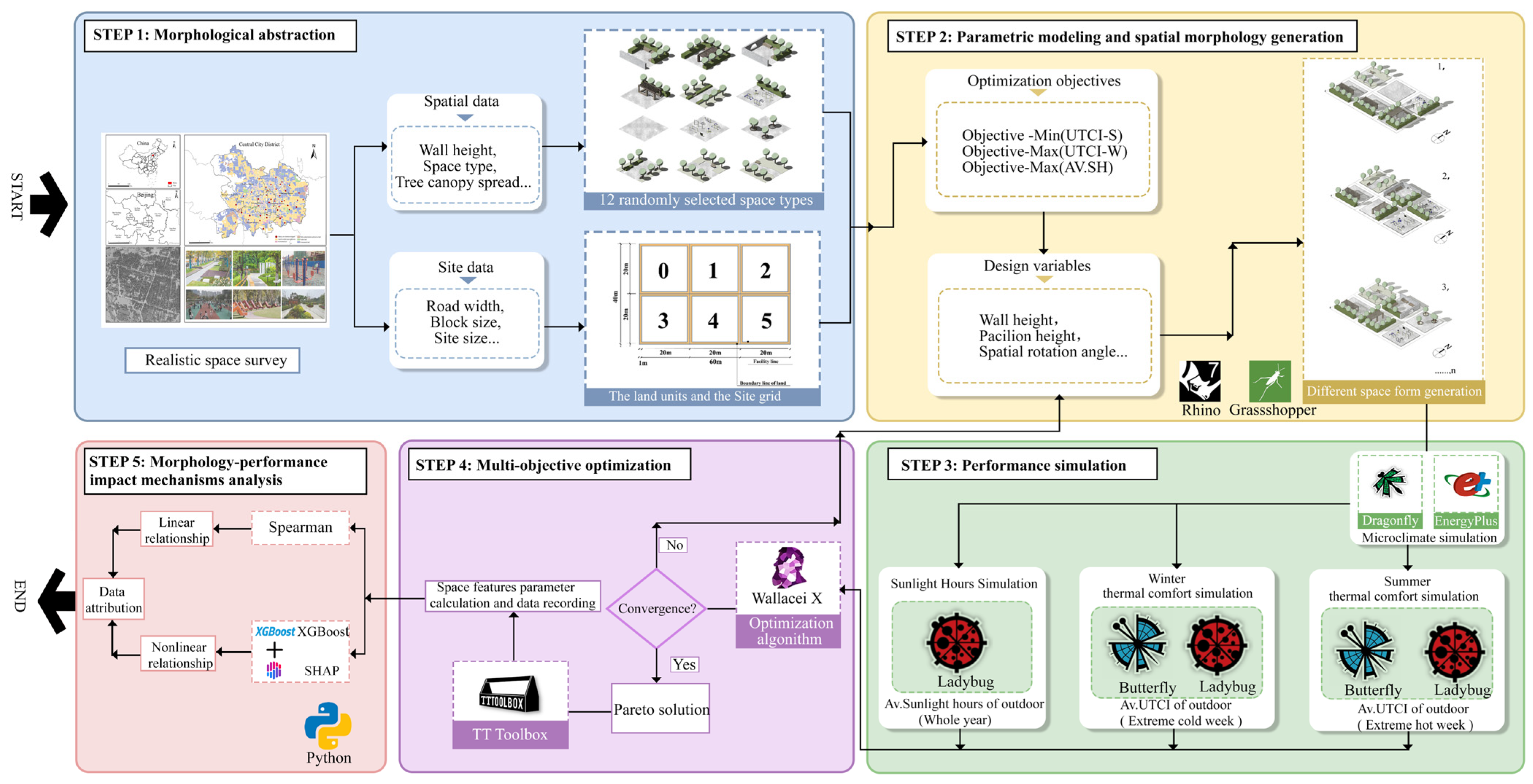
Figure 1. The study’s workflow.
Ijgi 14 00211 g001
Figure 2. The study area and survey points.
Ijgi 14 00211 g002
Figure 3. The 12 community activity space types derived from the empirical survey data.
Ijgi 14 00211 g003
Figure 4. Generation mechanism schematic.
Ijgi 14 00211 g004
Figure 5. Visualization of the morphological indicators.
Ijgi 14 00211 g005
Figure 6. The distributions of optimization solutions: (a) 3D spatial distribution of Pareto solutions; (b) distribution of Pareto solutions for the UTCI-S and UTCI-W indicators; (c) distribution of the Pareto solutions for the UTCI-S and AV.SH indicators; (d) distribution of the Pareto solutions for the AV.SH and UTCI-W indicators.
Ijgi 14 00211 g006
Figure 7. Comparison of data distributions between feasible and Pareto solutions for three optimization objectives: (a) UTCI-S; (b) UTCI-W; (c) AV.SH.
Ijgi 14 00211 g007
Figure 8. Comparison of the differences in spatial type selection between feasible and Pareto solutions: (a) feasible solutions; (b) Pareto solutions.
Ijgi 14 00211 g008
Figure 9. Correlation coefficient heatmap (values range from 1 to −1; higher absolute values indicate stronger correlations).
Ijgi 14 00211 g009
Figure 10. RF and SHAP interpretable machine learning model results: (a) bar plots of the UTCI-S; (b) summary plots of the UTCI-S; (c) bar plots of the UTCI-W; (d) summary plots of the UTCI-W; (e) bar plots of the AV.SH; (f) summary plots of the AV.SH.
Ijgi 14 00211 g010
Figure 11. ICE and PDP plots of CCR and CVH on UTCI-S: (a) ICE plot of CCR; (b) PDP plot of CCR; (c) ICE plot of CVH; (d) PDP plot of CVH.
Ijgi 14 00211 g011
Figure 12. PDP and ICE plots of OSR and AH on UTCI-W: (a) ICE plot of OSR; (b) PDP plot of OSR; (c) ICE plot of AH; (d) PDP plot of AH.
Ijgi 14 00211 g012
Figure 13. PDP and ICE plots of SVF on AV.SH: (a) ICE plot of SVF; (b) PDP plot of SVF.
Ijgi 14 00211 g013
Table 1. Design variable settings.
DimensionDesign VariableRangeUnitBaseline Remarks
Spatial MorphologyWall Height3 to 3.6m3.4Field research
Pavilion Height2.6 to 3m2.8Field research
Spatial Rotation Angle90, 180, 270, 360°-prioritizing symmetrical layout
Green LandscapeShrub Height0.5 to 1.2m0.8[78]
Shrub Width0.6 to 1.5m1Field research
Shrub Length<18m--
Ground Cover Area0 to 50% of total area%50Field research
Tree Height3.0 to 8.0m5Field research
Evergreen Tree Canopy Width (Summer)3.0 to 8.0m5Field research
Tree Canopy Width (Winter)with 10–15% crown width reduction in summer.m--
Number of Trees5 to 15points/100 m24[78]
Site FacilitiesFitness Equipment Category0, 1, 2, 3, 4, 5 --
Seat Height0.4 to 0.5m0.45[76]
Seat Length1.2 to 2.4m1.8
Seat Width0.35 to 0.45m0.4
Number of Fitness Equipment3 to 8 sets sets5[77]
Table 3. UTCI and AV.SH simulation parameter settings.
ParameterClassificationBoundary Condition SettingsBoundary Condition
UTCIClimate data-Modified EPW File
Time scaleSimulation PeriodExtreme Hot/Cold Week
Plant shadingCrown Width0.4
Tree Height0.8
Ground Reflectance0.4
Virtual Wind tunnelComputational Domain Boundary15 Hspace × 10 Hspace × 5 Hspace
Ground Roughness Length0.5
Atmospheric Boundary Layer Thickness450 m
Solid SurfaceNo-Slip Wall
Boundary ConditionsSymmetry Boundary
Outlet BoundaryStatic Pressure 0 Pa
Grid Cell Expansion Ratio1.1
Monitoring Grid Spacing2
Monitoring Point1.5 m
AV.SH Simulation
Period
Fromjan.1todec.31
Time ScaleMonitoring Point LocationGround Surface
Monitoring Point Height1.5 m
Monitoring Grid4 × 8
Table 4. Genetic Algorithm Parameter Settings.
Generation SizeGeneration CountCrossover ProbabilityMutation Distribution Index
50600.920
Disclaimer/Publisher’s Note: The statements, opinions and data contained in all publications are solely those of the individual author(s) and contributor(s) and not of MDPI and/or the editor(s). MDPI and/or the editor(s) disclaim responsibility for any injury to people or property resulting from any ideas, methods, instructions or products referred to in the content.