Walking to Public Transport: Rethinking Catchment Areas Considering Topography and Surrogate Buffers

Abstract

Service, or catchment areas of public transport stops are traditionally assessed using Euclidean or network distances, often neglecting other relevant factors such as topography. This study proposes a refined approach that integrates network-based accessibility with terrain variations and the effect they have on walking time and on the physical effort required for pedestrian movement. Using geographic information systems-based analysis that include walking time and walking energy cost models, the impact of topography on accessibility to public transport is evaluated in a case study of the hilly city of Coimbra, Portugal. Results show that, as compared to their flat counterparts, network distance-based service areas that consider hilliness, exhibit a decrease in accessibility of circa 10% in terms of area covered and population affected. These findings highlight the need for more realistic accessibility assessments to support more realistic and equitable public transport planning. Because extensive network datasets are not always available to decision-makers, this article also introduces the concept of surrogate buffers as a practical alternative for obtaining catchment areas, summarized by the “0.7/0.6R rule”.

1. Introduction

Public transportation plays a vital role in promoting sustainable and efficient urban mobility, offering benefits such as reduced congestion, lower environmental impact, and improved accessibility. Beyond its functional advantages, public transit fosters social inclusion by connecting everyone to education, healthcare, employment, and leisure opportunities, while also bridging social disparities and promoting equitable mobility through the expansion of active travel modes [1,2,3,4]. Social cohesion is closely tied to access to daily destinations, as greater distances—particularly when perceived as long—can weaken community ties [5]. To counteract this, planning strategies that enhance local accessibility to services and amenities are crucial in fostering inclusive and connected communities, promoting walkable, dense and diverse neighborhoods [6,7,8,9]. Measures such as subsidized public transportation, inclusive urban planning, and improved safety in the face of pandemics are essential to ensuring that public transportation systems attract new users and benefit everyone [10,11,12,13].

With the increased interest on promoting policies that seek to reduce vehicle emissions, reduce transport energy consumption, improve air quality, and encourage active lifestyles, enhancing pedestrian connections to transit stops is essential in maximizing investments in public transportation [14,15]. Beyond its environmental and mobility benefits, public transportation also promotes physical activity by incorporating walking into daily routines. If distances to public transportation stops are small enough to walk, these trips can incorporate regular physical activity that can lower the risk of chronic diseases [16,17]. Health-related organizations recommend at least 150 min of moderate physical activity per week [18,19,20], and a study in Montreal found that just by using public transport, travelers can achieve 54% of their daily recommended activity [21].

One of the key challenges in making public transportation a viable alternative to private motorized transport is its inherent limitation in providing door-to-door service. The first- and last-mile trips that are characteristic of public transportation play a crucial role in the attractiveness and accessibility of transit systems [22], and a competitive transportation system must address this challenge by ensuring seamless, convenient, and efficient access to the network [14], as these factors can significantly impact travel choice. Physical access to a transit stop is primarily assessed by the proximity of a passenger’s origin or destination to the nearest stop [23,24], often involving a short walk [25] and indeed the literature has confirmed that shorter walking distances increase public transportation use [26,27]. Thus, accurately defining catchment areas to transit stations is essential to estimate potential users, by measuring the population, urban facilities, and jobs within a given distance from stops [28,29]. The extent to which public transport serves these areas depends on walking distances, availability of suitable walking pathways, built environment characteristics, and transit service attributes such as stop spacing, frequency, and connectivity [30,31,32,33,34].

This study focuses on the accurate measurement of transit stop catchment areas. For that purpose, it compares four methods for measuring those areas: (a) straight line or Euclidean distance, a simple circular buffer that often overestimates accessibility and is used in this article for comparison; (b) network distance, i.e., distance traveled along the street network, which offers a more realistic approximation of actual movement; (c) walking time with inclines, a variant of network distance that accounts for changes in walking speed caused by terrain slope; and (d) energy expenditure with inclines, another variant of network distance that considers the metabolic effort required to traverse different slopes. The four methods are tested for the new Bus Rapid Transit (BRT) system in the city of Coimbra, Portugal, using geographic information systems (GIS) to analyze how each approach influences accessibility measurements. By comparing catchment areas based on these approaches, this research aims to identify the most precise method for defining transit catchment areas, providing insights for urban and transportation planning.

This research also presents the concept of surrogate buffers, which is a simpler, practical approach to obtaining catchment areas and ascertains whether these buffers can be a viable alternative to the more precise but technically more demanding methods. Surrogate buffers fill a literature gap of simple alternatives to network distance that can be easily implemented by municipal decision-makers.

Literature Review

The literature has previously established that circular buffers, e.g., simple circles around transit stops, usually with 600 m radii [35], may be suitable for basic analyses but are prone to overestimating accessibility by overlooking pedestrian network details. The circular buffer approach simplifies access distance to a straight-line measure, assuming that people enter stations straightly disregarding the complexities of the actual pedestrian road network and the geography and topography surrounding the stops [36]. Such inaccuracies can result in ineffective transit planning and a failure to meet the true needs of the community. In contrast, service areas methods that incorporate the pedestrian network accurately delineate accessible areas and exclude physically inaccessible zones within the circular buffer [37,38,39,40]. This disparity between network and straight line distances, whose quotient is sometimes referred to as the ”detour index” [41,42,43], is what often leads to considerably different catchment areas. However, a research gap remains, in that the authors above noticed the detour, but did not suggest any simple alternative to network distance to derive more accurate catchment areas. Addressing this gap is one of the objectives of the present research.

Some authors studied the effect of topography on catchment areas, mostly by including it in walkability indices. Examples include Rahman [44], who developed a microscale walkability index and applied it to catchments, having found an adverse effect of topography on walkability and pedestrian counts; Jeong et al. [45], who proposed a walkability index specific to public transport accessibility and used it to locate hub stations; Coelho et al. [46], who proposed a methodology to obtain bus service levels based on applying slope-dependent penalties to network distances; and Ceder et al. [47], who designed a methodology to optimize public transport stop locations in areas with challenging topography, by examining how gradients affect walking speed, the attractiveness of walking routes, and vehicle acceleration. However, these authors did not compare flat vs. non-flat catchment areas, e.g., via area size or population coverage rates, so the effect of topography remained unclear, making their methodologies unattractive for practical use.

It is the work of Macias [14] that bears the most resemblance to the present research. That author derived explicit pedestrian catchment areas for 12 stations of the metro expo line in Los Angeles, USA, a dense urban environment with low-to-moderate hilliness. Macias applied five different methods for deriving catchment areas: Euclidean distance (buffers), network distance, energy expenditure, travel time, and a combination of time and energy that also included some features of the infrastructure. The aim was to ascertain whether the respective catchment areas significantly differ in terms of land and transport characteristics, having found they do differ in terms of area and street and sidewalk density. The present article focuses more on area and population coverage and applied a similar methodological approach, in that explicit catchment areas were also derived using four methods like those of Macias. Euclidean distance (buffers) and (flat) network distance were calculated the same way as Macias [14], and energy was calculated using the more recent expenditure formula from Minetti et al. [48]. Travel time, however, was calculated in a very different way. While Macias obtained travel-time catchment areas considering waiting times at crossings, this article uses travel time as an indirect measurement of the impact of topography. This was carried out by reflecting the effect of slope on walking speed and deriving the corresponding service areas of BRT stops.

In summary, while there is research exploring more precise methods for defining public transportation catchment areas, it remains in its early stages, as Hayauchi et al. [49] recognize. This article fills some of the gaps in this field: Firstly, it derives explicit catchment areas that reflect the impact of topography in two ways: using travel time, corrected for inclines; and energy expenditure, expanding on previous work by Macias [14]. These are then compared to the corresponding catchment areas for flat terrain to determine the significance of topography. Secondly, it proposes an alternative method to obtain catchment areas that emulates the results of precise network-based measures without the need for specialized tools. This method, the so-called surrogate buffer method, trades a small amount of precision for a quick and practical way to obtain catchment areas that can be very appealing to municipal planners.

2. Methodology

The section above makes it clear that accurate treatment of public transport catchment areas must go beyond simple Euclidean distance. Accordingly, the methodology considers network distance and two measures that relate to topography: walking time to stops, modified for inclines, and metabolic energy expenditure. For comparison, Euclidean distance was also considered. The derivations below are described using ArcGIS commands, but any other GIS environment can be used, provided it has the tools to execute the same operations. Three GIS datasets need to be acquired for the methodology: public transport stops, walking network, and population distribution, the last of which can be expressed in various forms, e.g., buildings with number of inhabitants, fishnet and centroids thereof with population information, etc.

2.1. Catchment Area Derivation Methods

2.1.1. Euclidean and Network Distance

The Euclidean distance service area to a set of points is defined as the union of the individual service areas of each stop. When the set of points are public transport stops, the service areas are often called ”catchment areas”. The individual service areas of radius R can be obtained using the ArcGIS buffer tool (to a set of points) and their union is formed with the merge command.

Network distance service areas of size R are obtained using the Network Analyst extension (service area tool with impedance as distance and default break R), followed by merge. Service areas obtained this way are not corrected for topographic effects and reflect the status quo as if the city were flat. Hence, they are called ”flat service areas”.

2.1.2. Walking Time with Inclines

The impact of topography can be studied via the extra time inclines have on walking speed. The extensive work of Campbell et al. [50] provides data-driven results on how walking speed depends on the grade. If inclusive planning of the walking infrastructure is sought, those authors recommend using the Lorentz probability distribution 5% quantile that relates walking speed (m/s) to incline (in degrees) as

$$v_{\mathrm{walk}}\left(\theta \right)=36.813\left({\displaystyle \frac{1}{14.041\pi \left(1+{\left(\frac{\theta +1.527}{14.041}\right)}^2\right)}}\right)+0.320-0.00273\theta$$

(1)

where the numeric figures are least-squares fitted values for the Lorentz distribution parameters. For reference, an incline of $\theta =0^{\mathrm{o}}$ yields $v_{\mathrm{walk}}\left(\theta \right) \approx 1.145{\displaystyle \frac{\mathrm{m}}{\mathrm{s}}}$, which is about 82% of Tobler’s [51] estimate of 1.4 m/s for average walking speed on the flat. Using ArcGIS field calculator, Equation (1) can be applied to endow the walking network arcs with slope-dependent walking speed information, from which traveling time (s) can be derived as $t={\displaystyle \frac{l}{v_{\mathrm{walk}}\left(\theta \right)}}$, with $l$ the arc length (m). A buffer of radius R would require $t_R={\displaystyle \frac{R}{v_{\mathrm{walk}}\left(0\right)}}$ to walk through, so service areas for walking times considering inclines require deriving those areas using time as impedance and $t_R$ as threshold (ArcGIS default break), which can be performed with the ArcGIS network analyst once the walking network is given information on (slope-dependent) arc traversing times. If plotted, Equation (1) exhibits a monotonous decrease in walking speed with positive slope, whereas for negative slopes speed increases slightly, topping out at $v_{\mathrm{walk}}\left(-1.845\right)\approx 1.159{\displaystyle \frac{\mathrm{m}}{\mathrm{s}}}$, and subsequently decreases due to the necessity to brake.

2.1.3. Energy Expenditure with Inclines

Topography also impacts metabolic energy spending when walking. Since this expenditure is non-linear with walking speed or arc incline, a specific model for the dependence must be applied to network arcs. Minetti et al. [48] provides one such model, a fifth-order polynomial regression whose expression is

$$E_{\mathrm{walk}}\left(s\right)=280.5s^5-58.7s^4-76.8s^3+51.9s^2+19.6s+2.5$$

(2)

where, again, the numeric figures are least-squares fitted values for the fifth-order polynomial. Units for this formula are $E_{\mathrm{walk}}$ in J/kg.m and $s$ the slope quotient $\Delta y/\Delta x,$ which is negative going downhill. A healthy 80 kg person would spend circa $2.5\times 80=200 \mathrm{J}$ per each meter walking on the flat, so a walk of radius R (in meters) requires 200R joules of energy expenditure. This is metabolic energy, i.e., all the energy transformed by the body, including basal metabolism, heat production, and muscular mechanical work. After endowing the walking network with the (slope-dependent) energy expenditure information given by Equation (2), deriving service areas for walking energy expenditure of a buffer or radius R can be performed in the ArcGIS network analyst with expenditure as impedance and 200R joules as threshold. Similar to time, expenditure increases with positive slope, slightly decreases with negative slope, minimizing locally at $E_{\mathrm{walk}}\left(-0.125\right)=0.9355{\displaystyle \frac{\mathrm{kJ}}{\mathrm{kg}.\mathrm{m}}}$. Being a regression formula, it is not very reliable for extrapolating when slopes are greater than 1 or smaller than −0.5.

The flat travel time and energy methods all use the actual walking network for calculations and are therefore deemed collectively as ”network distance-based methods”.

2.2. Combining Toward and Away Catchment Areas

The vast majority of the time, travelers must make two walking trips between residences and public transport stops: a trip toward the stop, and a return trip (away from the stop). These trips usually follow the shortest distance route, so they are the same route, traversed in opposite directions when going toward/away. However, if topography is considered, the two trips might feel very different. What may be a pleasant downhill promenade toward the stop may become an annoyance when going uphill back home. Thus, a catchment area can only be considered as such if both the toward and away trips are convenient enough to be carried out walking. For this reason, toward and away service areas for time and energy with inclines should be derived and their overlap obtained. This can be carried out in ArcGIS with the intersect tool and that intersection is henceforth called ”travel time w/inclines” and ”energy expenditure w/inclines” catchment areas.

3. Case Study

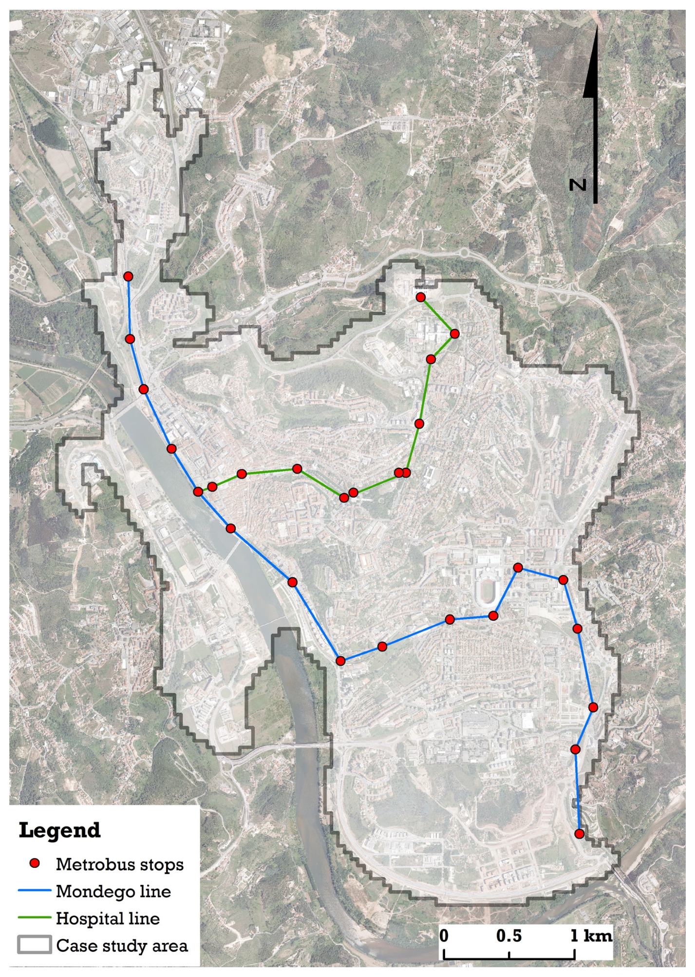
The proposed methodology was applied to a case study, the city of Coimbra, Portugal. This is a mid-sized city in the middle of the country with healthcare and higher education as main economic activities. The study area focuses on the center of Coimbra, a very hilly urban environment that hosts 49,066 inhabitants (the whole city has about double that) and spans an area of 14.45 km². By the time of writing, Coimbra is undergoing development of a bus rapid transit (BRT) system, nicknamed “Metrobus”, that will connect nearby municipalities to Coimbra and various locations within the city. The public transport stops in the case study refer to this mobility system. The stops are closer together than those of the metro expo line referred to by Macias, leading to overlaps in individual catchment areas, a feature that did not exist in that earlier study.

The Metrobus is expected to substantially change the modal split in Coimbra, which is currently very dependent on private cars for trips longer than walking distance, ranging from 60% to 80%, depending on trip purpose (higher for commuting trips). The walking mode ranges from 10% to 40%, again depending on trip purpose and user profile (younger people tend to walk more, mainly to school), and public transport oscillates between 12% and 25% (lower for commuting purposes) [52]. Figure 1 shows the study area and location of Metrobus stops; the necessary GIS datasets are described in

Table 1. Case study datasets.

Dataset	Type	Role
BRT stops	Points feature class	Facilities for catchment area calculations
Inhabitants	Points feature class	Location of inhabitants (buildings) for coverage calculations
Walking network	Polyline feature class	Network dataset with altimetric information

below. The study area spans an area of 14.45 km² and hosts 49,066 inhabitants. The hospital line contains three instances of bus stops next to each other. These are actually the same stop, with two drop-off points on opposite sides of the street, each serving a specific bus traffic direction.

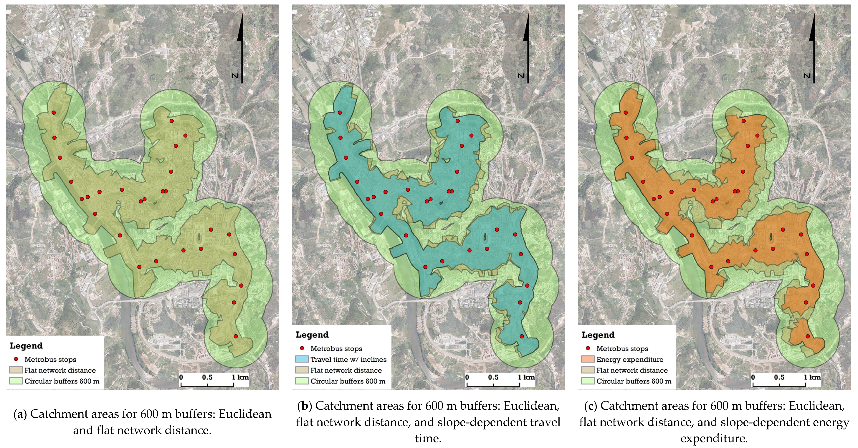
From the altimetry information on the walking network, Equations (1) and (2) were applied to each arc using field calculator and the output was loaded onto the network’s associated table. Afterward, service areas to the Metrobus stops were obtained using buffers, network (flat) distance, and time and energy expenditure as impedance. Following the literature guidelines mentioned in the literature review section, the chosen radius for the buffer was R = 600 m. This translates into the same 600 m network flat distance, 524 s time threshold, and 120 kJ energy threshold.

Results

Figure 2a shows the results for the Euclidean (buffer) and network flat-distance service areas. This figure exhibits the typical mismatch between the two approaches to service areas reported in the literature (e.g., Andersen and Landex [37], Macias [14]), with Euclidean buffers being overly optimistic in how wide-reaching the catchment area is.

Figure 2b,c add time and energy expenditure service areas to the information shown in Figure 1. Recall these two are the intersection of toward and away service areas. Separate results for each travel direction are available in Supplementary Materials, Figures S1 and S2. For travel time, it can be seen that topography does have an impact on the catchment area coverage as compared to flat terrain. For energy, this impact appears to be greater.

Figure 2 displays the area differences between the various ways to obtain catchment areas to Metrobus stops. Another indicator that is perhaps more important is how many people are affected by those differences. Using the ArcGIS intersect tool between the various service areas and the population location feature class, that effect can be calculated.

Table 2. Summary statistics on catchment areas and inhabitants covered.

Catchment Area Type (600 m)	Area [km2]	Inhabitants Covered	% of Study Area	% of Buffer Area	% of Flat Dist. Area	% of Study Area Pop.	% of Buffer Area Pop.	% of Flat Dist. Area Pop.
Buffer	12.96	36279	90%	100%	N/A	74%	100%	N/A
Flat network distance	7.00	24809	48%	54%	100%	51%	68%	100%
Travel time w/inclines	6.22	21515	43%	48%	89%	44%	59%	87%
Energy expenditure w/inclines	5.31	17829	37%	41%	76%	36%	49%	72%

summarizes the results concerning catchment area coverage and population covered.

In reading Table 2, the percentage columns are calculated in relation to the quantity on top. For instance, the union of all catchment areas of travel time spans an area that is 43% of the study area (6.22/14.45); catchment areas of flat network distance span an area that is 54% of the area spanned by catchment areas of Euclidean buffers (7.00/12.96); catchment areas of energy expenditure span an area that is 76% of the area spanned by catchment areas of flat network distance (5.31/7.00), and so forth. The same goes for the population percentage columns. For instance, catchment areas of travel time span an area that includes 59% of the population covered by Euclidean buffers (21515/36279), etc.

Table 2 shows that the largest differences occur in going from buffer to network distance, with catchment areas reducing by nearly one-half (100% to 54%) and population coverage reducing by about one-third (100% to 68%). This result approximates that reported by Macias [14], although it is not as pronounced as the reduction found by that author, namely, 100% to 43%.

The impact of topography, as measured by travel time, further decreases catchment area size and population coverage by roughly another 10%. When measuring topography impact by energy expenditure, this decrease is more pronounced, approximately 25%. Macias also provided estimates for catchment area reductions due to energy expenditure considerations, the outcome being somewhat different: a 6% decrease rather than 25%. This could be due to different local topography, or the fact that Macias used an energy expenditure estimation method other than Equation (2).

The fact that population coverage is less affected by topography than the size of catchment areas may indicate that the Metrobus lines run along densely populated zones, lessening the effect of using a cruder measure such as a buffer.

4. Discussion

The results reveal two main conclusions: firstly, and confirming previous findings in the literature, the reduction in going from the standard practice buffer analysis into a network-based analysis has a major impact in estimating the coverage of catchment areas, be it in area size or population. Secondly, in cities where the terrain is not flat, topography significantly affects that estimation. Albeit, it is a smaller role compared to the buffer-to-network distance decrease, it is nevertheless significant and impacts both catchment area size and population covered in similar ways. Focusing on travel time, a reduction of 10–15% in coverage as compared to the flat case is generally expected and municipal decision-makers are well advised not to disregard this aspect. After all, if these authorities are willing to change from simple (but quick) estimation methods such as circular buffers, they might as well take the opportunity to consider other aspects that enter the fray.

The difference between topography affecting travel time as compared to energy expenditure also raises the question of which indicator might be more representative, as the impact on energy appears to be more pronounced. To address this point, note that walking is a low-intensity physical activity. Walking at regular speed on flat ground requires an expenditure of 2–3 METS (metabolic equivalent of task; 1 MET = 1.162 W/kg = person at rest) and going up street-grade inclines can raise this intensity to 4–5 METS [48]. Higher inclines, such as those of stairways, require upward of 9–10 METS. The threshold for the anaerobic regime sits at about 6–8 METS [53], so long stretches of stairways may trigger a transition to that regime, in which the body starts to build up lactate in the blood, leading to discomfort and the need to stop after a while. However, since street-grade inclines rarely require raising metabolic rates to such high levels, in practice, the traveler has a tolerance for increasing his or her walking energy expenditure without feeling discomfort. Indeed, it is known that cycling requires about twice the energy of walking (4–6 METS) [54] and people routinely carry out that activity without undergoing the aerobic–anaerobic transition, spending twice the energy as they would walking (and, incidentally, going four to five times farther). In other words, it is not the total (cumulative) energy expenditure that determines whether a person needs to stop from tiredness, but the way that expenditure is delivered, i.e., the metabolic power developed. As long as one does not cross the anaerobic threshold, it is fine to increase energy expenditure. These considerations suggest that the catchment area results obtained from energy expenditure may be too pessimistic and that travel-time figures are more accurate.

A Surrogate Buffer-Method Proposal

Given the popularity buffer analysis has in transport planning, it is worth considering whether buffers of a smaller radius, i.e., ”surrogate buffers”, can somehow emulate the results that network-based analyses produce. For this purpose, buffer radii can sequentially be reduced and the corresponding area covered recalculated, the procedure being repeated until the buffer coverage area is similar to that of a network-based approach. Then, to evaluate how well the new (reduced radius) buffer coverage matches the network-based coverage, the two can be intersected to obtain a visual impression of the overlap and statistics of the quality thereof.

This method was applied to find surrogate buffers for flat network distance, time travel, and energy expenditure catchment areas. Figure 3 and Figure 4 below show a map outcome of the procedure and

Table 3. Summary statistics for surrogate buffers of 600 m buffers (area equivalence).

Catchment Area Type (600 m)	Real Area [km2]	Real Inhab.	Surr. Buffer Radius [m]	Surr. Buffer Area [km2]	Surr. Buffer Area Inhab.	Area Overlap and Quality Q (%)	Inhab. Overlap and Quality Q (%)
Flat network distance	7.00	24,809	345 (58%)	7.00 (100%)	20,227 (82%)	5.66 (81%)	19,242 (78%)
Travel time w/inclines	6.22	21,515	315 (53%)	6.23 (100%)	18,404 (86%)	4.99 (80%)	16,901 (79%)
Energy expenditure w/inclines	5.31	17,829	280 (47%)	5.29 (100%)	16,003 (90%)	4.20 (79%)	14,136 (79%)

provides summarizing statistics. The index Q is a measure of the quality of the overlap between circular buffers and catchment areas based on network-based methods, i.e., how well the two match. It is defined by $Q={\displaystyle \frac{\mu \left(A\cap B\right)}{\max \left\{\mu \left(A\right),\mu \left(B\right)\right\}}}$, with $\mu \left(x\right)$ the measure of set $x$, and area in km² or number of inhabitants. Note that overlap quality can only be 100% if $A \subseteq B$ (or $A \supseteq B$) and $A$ and $B$ have the same measure.

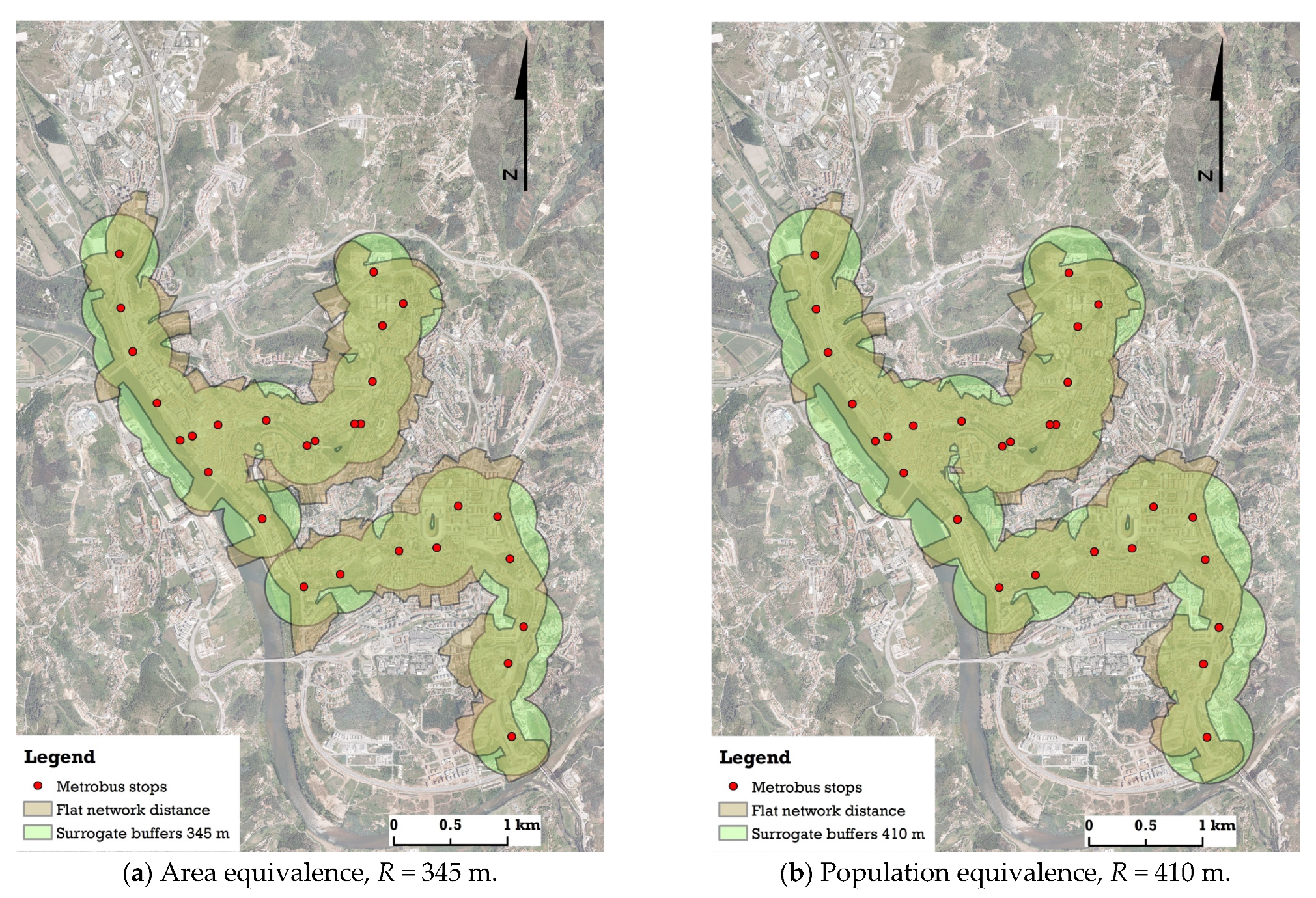
Table 3 reads as follows: for instance, entry “345 (58%)” means that if surrogate buffers are created such that the union of their areas equals that of the union of flat-network-distance real catchment areas, then the surrogate buffers should have a radius of 345 m, which is 58% of a Euclidean buffer of 600 m radius. Entry “18,404 (86%)” means that surrogate buffers for travel time include 18,404 inhabitants, which is 86% of those covered by the real network-based travel-time catchment areas (21,515). Entry “14,136 (79%)” means that the overlap of real and surrogate buffers of energy expenditure cover 14,136 inhabitants, corresponding to a quality index of 79% (14,136/17,829). And so forth.

The surrogate buffer catchment areas cover, by design, the same areas of those obtained with precise network-based calculations, albeit with a different shape, as Figure 3a and Figure 4a show (see Supplementary Figure S5a for energy expenditure). Surrogate buffers produce a trade-off, where pieces of the network-based catchment areas are replaced by bits of the buffer circles. By itself this has no special meaning. What is meaningful for transport planning is whether this trade-off can capture demand (i.e., inhabitants) adequately. Table 3 provides guidance to this: surrogate buffers underestimate demand by roughly 10–20%, so there will be more people reaching the Metrobus stops than what the surrogate buffers suggest.

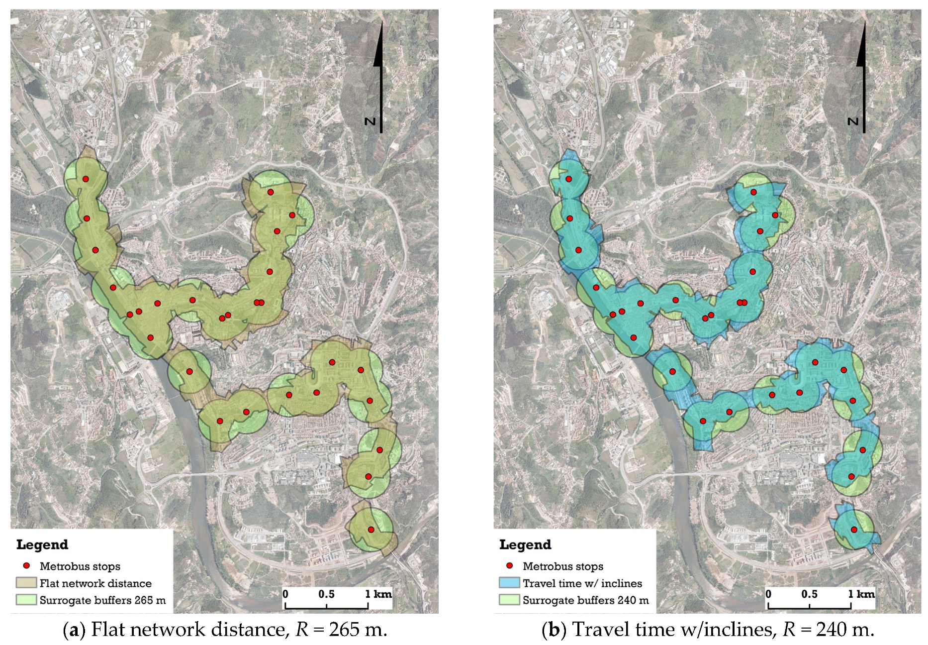
To compensate for the underestimation of population coverage, alternative surrogate buffers can be obtained by defining a radius for matching number inhabitants, rather than matching area coverage. Repeating the procedure for this objective yields the maps shown in Figure 3b and Figure 4b (see Supplementary Figure S5b for energy expenditure) and the results reported in

Table 4. Summary statistics for surrogate buffers of 600 m buffers (population equivalence).

Catchment Area Type (600 m)	Real Area [km2]	Real Inhab.	Surr. Buffer Radius [m]	Surr. Buffer Area [km2]	Surr. Buffer Area Inhab.	Area Overlap and Quality Q (%)	Inhab. Overlap And Quality Q (%)
Flat network distance	7.00	24,809	410 (68%)	8.60 (123%)	24,639 (99%)	6.40 (76%)	22,376 (90%)
Travel time w/inclines	6.22	21,515	360 (60%)	7.38 (119%)	21,324 (99%)	5.55 (75%)	18,694 (87%)
Energy expenditure w/inclines	5.31	17,829	305 (51%)	5.96 (112%)	17,617 (99%)	4.51 (76%)	15,086 (85%)

. (Note: the equivalent of Figure 3 and Figure 4 for energy expenditure were moved to Supplementary Materials because, as argued, energy expenditure is not as accurate a predictor of slope impact as travel time).

Table 4 shows that surrogate buffers for equivalent coverage of population work better, not only because they are designed around population coverage, a more meaningful impact measure, but also because they yield better overlap quality Q with the actual network-based measures (slightly worse area overlap quality, but considerably better inhabitant overlap quality).

Table 4 also suggests a practical rule for dimensioning surrogate buffers. Before elaborating on this rule, and to solidify its guideline, a similar analysis was made for other commonly used buffer radii, namely 400 m and 800 m (quarter-mile and half-mile buffers) [55,56]. The results are given in Figure 5 and Figure 6 (Figure 7 repeats 3b and 4b for convenience) and

Table 5. Summary statistics for surrogate buffers of 400 m buffers (population equivalence).

Catchment Area Type (400 m)	Real Area [km2]	Real Inhab.	Surr. Buffer Radius [m]	Surr. Buffer Area [km2]	Surr. Buffer Area Inhab.	Area Overlap and Quality Q (%)	Inhab. Overlap and Quality Q (%)
Flat network distance	4.46	14,812	265 (66%)	4.88 (109%)	14,941 (101%)	3.76 (77%)	12,976 (87%)
Travel time w/inclines	4.00	12,818	240 (60%)	4.21 (105%)	12,927 (101%)	3.28 (78%)	10,997 (85%)
Energy expenditure w/inclines	3.56	11,326	220 (55%)	3.67 (103%)	11,389 (100%)	2.83 (77%)	9208 (81%)

and

Table 6. Summary statistics for surrogate buffers of 800 m buffers (population equivalence).

Catchment Area Type (800 m)	Real Area [km2]	Real Inhab.	Surr. Buffer Radius [m]	Surr. Buffer Area [km2]	Surr. Buffer Area Inhab.	Area Overlap and Quality Q (%)	Inhab. Overlap and Quality Q (%)
Flat network distance	9.12	34,408	560 (70%)	12.07 (132%)	34,353 (100%)	8.53 (94%)	32,172 (94%)
Travel time w/inclines	8.36	30,807	505 (63%)	10.8 (129%)	30,717 (100%)	7.76 (93%)	28,263 (92%)
Energy expenditure w/inclines	7.14	25,091	415 (52%)	8.72 (122%)	25,143 (100%)	6.33 (87%)	21,812 (87%)

. The corresponding maps for energy expenditure can be found in Supplementary Materials, Figures S6c, S7c, and S8c.

Looking at the surrogate buffer radii for catchment areas of 400 m, 600 m, and 800 m Euclidean distance, Table 4, Table 5 and Table 6, considering flat network distance and travel time with inclines, it is seen that the network distance-based catchment areas can be effectively represented by surrogate buffers of sizes 66–70% of the original radius for the flat case and 60–63% considering inclines, with good quality indicators Q. For making practical decisions, the implications of these findings suggest the following recommendation for municipal authorities, which can be referred to as the “0.7/0.6R rule”:

When planning for catchment areas of public transport stops, if GIS technology or adequate datasets are not available, consider doing buffer analysis of radius 0.7R, where R is the radius originally proposed. If the city is hilly, consider instead 0.6R.

This recommendation mimics the effect of network distance and hilliness and captures the population involved within reasonable precision while keeping the simplicity of circular buffers. Note that circular buffer approaches allow for straightforward on-the-fly procedures, such as compass and ruler drawing of catchment areas on a paper map, which is one of the reasons for its popularity.

5. Conclusions

Catchment areas for public transportation stops are a fundamental tool in transport planning that are used to determine how accessible transit services are to the surrounding population. However, there are multiple ways to calculate these areas, each with different implications for planning decisions. This research studied the impact of topography on catchment areas by comparing four approaches for obtaining those areas—radius-based (buffer), flat network distance, travel time with inclines, and energy expenditure with inclines. The findings reveal that while the change in going from buffer analysis to network-based analysis has the most impact, considerably reducing catchment area size and population coverage, topography has a non-trivial effect, further reducing that size by roughly 10%.

Currently, many municipal authorities still rely on a radius-based approach, defining accessibility as all locations within a 600 m straight-line buffer distance of a transit stop. However, this method is deeply flawed, as it fails to account for the actual street network, often including areas that are not truly reachable within 600 m of walking. This misrepresentation leads to overestimated accessibility and poor decision-making in transit planning, a problem that is magnified in hilly cities due to the impact of slopes in travel-time energy expenditure. A network-based approach with inclusion of topographic effects provides a far more accurate measure of accessibility and a shift to these methods would be important for ensuring public transport planning reflects real-world accessibility conditions.

While a network-based approach provides a more nuanced understanding of accessibility—especially in hilly areas—it also requires more complex calculations and specialized GIS tools that require adequately curated datasets. This is why the radius-based buffer approach remains popular in practical decision-making at the municipal level. This research showed that it is possible to continue using this popular method to obtain catchment areas if buffer sizes are judiciously selected. Indeed, precise network-based calculations yield very similar results to radius-based calculations for reduced buffer sizes of 0.7R or 0.6R for hilly cities, where R is the desired engineering guideline used in transport planning, usually 400 m, 600 m, or 800 m. This recommendation, i.e., the surrogate buffer method, and the finding that catchments area sizes reduce by approximately 10% in hilly cities, are the main contributions of this article.

Concerning drawbacks and limitations of this research, the drawback of surrogate buffers is that they are an approximation to the actual situation: surrogate buffers trade simplicity for precision. The main limitation is that only one case study was analyzed. The proposed “0.6/0.7R” rule requires further validation to move from a data-driven suggestion to an established engineering guideline; thus, future work should include analyzing more cities using the methodology proposed herein, preferably hilly ones. Furthermore, since the case study was carried out in a developed country, it would also be important to include cities from developing countries, where public transport systems are often inadequate. The definition of “hilly city” may also require a more rigorous debate in the future, as currently the definition is very much subjective and open to researcher sentiment.

For greater refinement, more factors that influence walkability can be included in the network-based methods. For instance, poor condition of the walking infrastructure may deter some people from walking to public transport stops. Assessing this condition in the catchment areas would help understanding whether the problem may arise (see, e.g., [57,58] for an assessment approach). Studying its actual impact on walking probability would then provide figures that could alter the geometry of catchment areas. Likewise, if long public stairways are abundant in a neighborhood, traveler tiredness may put more stringent restrictions on walking than travel time. We hope to address some of these issues in the near future.

References

- Ermagun, A.; Tilahun, N. Equity of Transit Accessibility across Chicago. Transp. Res. Part D Transp. Environ. 2020, 86, 102461. [Google Scholar] [CrossRef]
- Karner, A. Assessing Public Transit Service Equity Using Route-Level Accessibility Measures and Public Data. J. Transp. Geogr. 2018, 67, 24–32. [Google Scholar] [CrossRef]
- Nazari Adli, S.; Chowdhury, S.; Shiftan, Y. Justice in Public Transport Systems: A Comparative Study of Auckland, Brisbane, Perth and Vancouver. Cities 2019, 90, 88–99. [Google Scholar] [CrossRef]
- Zinia, F.A.; Bhandari, P.; Tuffour, J.P.; Hong, A. Evaluating Social Equity of Transit Accessibility: A Case of Salt Lake County, U.S. Transp. Res. Rec. 2023, 2677, 806–814. [Google Scholar] [CrossRef]
- Mombelli, S.; Miralles-Guasch, C.; Marquet, O. Can Proximity Forge Strong Bonds? Exploring the Relationship between Urban Proximity and Social Cohesion at the Neighbourhood Level. Sustain. Cities Soc. 2025, 119, 106096. [Google Scholar] [CrossRef]
- Monteiro, J.; Para, M.; Sousa, N.; Natividade-Jesus, E.; Ostorero, C.; Coutinho-Rodrigues, J. Filling in the Spaces: Compactifying Cities towards Accessibility and Active Transport. ISPRS Int. J. Geo-Inf. 2023, 12, 120. [Google Scholar] [CrossRef]
- Stojanovski, T. Urban Design and Public Transportation—Public Spaces, Visual Proximity and Transit-Oriented Development (TOD). J. Urban Des. 2020, 25, 134–154. [Google Scholar] [CrossRef]
- Nogueira, A.; Santos, B.; Gonçalves, J.; Kempa, J.; Chmielewski, J. Transportation Network Spatial Analysis to Measure Pedestrian Suitability. The Case of Hilly Cities. IOP Conf. Ser. Mater. Sci. Eng. 2021, 1203, 022107. [Google Scholar] [CrossRef]
- Shi, Z.; Zhou, C.; Cheng, L.; He, M.; Liu, Y. Examining Spatial Variations in Walking Activity Among Older Adults Considering the Impact of Topographical Characteristics. Transp. Res. Rec. 0(0) 2024. [Google Scholar] [CrossRef]
- Karel, M. Transport Justice: Designing Fair Transportation Systems; Routledge: London, UK, 2016; ISBN 978-0-415-63832-6. [Google Scholar]
- Kunskaja, S.; Budzyński, A. Sustainable Societal Transformation: Shaping Renewable Energy Technologies in Transport. MATEC Web Conf. 2024, 390, 01006. [Google Scholar] [CrossRef]
- Monteiro, J.; Sousa, N.; Pais, F.; Coutinho-Rodrigues, J.; Natividade-Jesus, E. Planning Cities for Pandemics: Review of Urban and Transport Planning Lessons from COVID-19. Proc. Inst. Civ. Eng.—Munic. Eng. 2023, 176, 125–138. [Google Scholar] [CrossRef]
- Ilham, I. The Impact of Regional Structure and Topography on the Effectiveness of Public Transportation Services. West Sci. Social. Humanit. Stud. 2024, 2, 2083–2092. [Google Scholar] [CrossRef]
- Macias, K. Alternative Methods for the Calculation of Pedestrian Catchment Areas for Public Transit. Transp. Res. Rec. 2016, 2540, 138–144. [Google Scholar] [CrossRef]
- Monteiro, J.; Sousa, N.; Coutinho-Rodrigues, J.; Natividade-Jesus, E. Challenges Ahead for Sustainable Cities: An Urban Form and Transport System Review. Energies 2024, 17, 409. [Google Scholar] [CrossRef]
- Djurhuus, S.; Hansen, H.S.; Aadahl, M.; Glümer, C. The Association between Access to Public Transportation and Self-Reported Active Commuting. Int. J. Environ. Res. Public Health 2014, 11, 12632–12651. [Google Scholar] [CrossRef]
- Veillette, M.-P.; Deboosere, R.; Wasfi, R.; Ross, N.; El-Geneidy, A. Small Steps, Big Differences: Assessing the Validity of Using Home and Work Locations to Estimate Walking Distances to Transit. Transp. Res. Rec. 2018, 2672, 840–848. [Google Scholar] [CrossRef]
- European Commission Physical Activity Recommendations for Adults. Available online: https://knowledge4policy.ec.europa.eu/health-promotion-knowledge-gateway/physical-activity-sedentary-behaviour-table-2b_en?utm_source=chatgpt.com (accessed on 14 February 2025).
- Office of Disease Prevention and Health Promotion Seasonal Strategies: Empowering Your Community to Stay Active—Even in the Colder Months. Available online: https://odphp.health.gov/news/202411/seasonal-strategies-empowering-your-community-stay-active-even-colder-months (accessed on 14 February 2025).
- World Health Organization Physical Activity. Available online: https://www.who.int/news-room/fact-sheets/detail/physical-activity (accessed on 14 February 2025).
- Mageau-Béland, J.; Morency, C. Assessing Physical Activity Achievement by Using Transit. Transp. Res. Rec. 2021, 2675, 506–514. [Google Scholar] [CrossRef]
- Li, L.; Bai, Y.; Song, Z.; Chen, A.; Wu, B. Public Transportation Competitiveness Analysis Based on Current Passenger Loyalty. Transp. Res. Part A Policy Pract. 2018, 113, 213–226. [Google Scholar] [CrossRef]
- Eboli, L.; Forciniti, C.; Mazzulla, G. Service Coverage Factors Affecting Bus Transit System Availability. Procedia—Soc. Behav. Sci. 2014, 111, 984–993. [Google Scholar] [CrossRef]
- Texas A&M Research Foundation Guidelines for the Location and Design of Bus Stops; Transportation Research Board–National Research Council: Washington, DC, USA, 1996; Available online: https://nacto.org/wp-content/uploads/tcrp_report_19.pdf (accessed on 14 February 2025).
- Murray, A.T.; Wu, X. Accessibility Tradeoffs in Public Transit Planning. J. Geogr. Syst. 2003, 5, 93–107. [Google Scholar] [CrossRef]
- Ewing, R.; Cervero, R. Travel and the Built Environment: A Meta-Analysis. J. Am. Plan. Assoc. 2010, 76, 265–294. [Google Scholar] [CrossRef]
- Tennøy, A.; Knapskog, M.; Wolday, F. Walking Distances to Public Transport in Smaller and Larger Norwegian Cities. Transp. Res. Part D Transp. Environ. 2022, 103, 103169. [Google Scholar] [CrossRef]
- García-Palomares, J.C.; Gutiérrez, J.; Cardozo, O.D. Walking Accessibility to Public Transport: An Analysis Based on Microdata and GIS. Environ. Plann B Plann Des. 2013, 40, 1087–1102. [Google Scholar] [CrossRef]
- van der Waerden, P.; van der Waerden, J.; Burger, M. Exploring the Role of Public Transport Service and Walking Route Related Factors to Identify Maximum Walking Distances to Bus Stops in the Netherlands. J. Public Transp. 2024, 26, 100096. [Google Scholar] [CrossRef]
- Noh, N.M.; Mohamad, D.; Hamid, A.H.A. Acceptable Walking Distance Accessible to the Nearest Bus Stop Considering the Service Coverage. In Proceedings of the 2021 International Congress of Advanced Technology and Engineering (ICOTEN), Online, 4–5 July 2021; pp. 1–7. [Google Scholar]
- Mulley, C.; Ho, C.; Ho, L.; Hensher, D.; Rose, J. Will Bus Travellers Walk Further for a More Frequent Service? An International Study Using a Stated Preference Approach. Transp. Policy 2018, 69, 88–97. [Google Scholar] [CrossRef]
- O’Connor, D.; Caulfield, B. Level of Service and the Transit Neighbourhood—Observations from Dublin City and Suburbs. Res. Transp. Econ. 2018, 69, 59–67. [Google Scholar] [CrossRef]
- van Soest, D.; Tight, M.R.; Rogers, C.D.F. Exploring the Distances People Walk to Access Public Transport. Transp. Rev. 2020, 40, 160–182. [Google Scholar] [CrossRef]
- Yang, R.; Liu, Y.; Liu, Y.; Liu, H.; Gan, W. Comprehensive Public Transport Service Accessibility Index—A New Approach Based on Degree Centrality and Gravity Model. Sustainability 2019, 11, 5634. [Google Scholar] [CrossRef]
- Calthorpe, P. The Next American Metropolis: Ecology, Community, and the American Dream; Princeton Architectural Press: New York, NY, USA, 1993; ISBN 978-1-878271-68-6. [Google Scholar]
- Chen, X.; Pei, T.; Song, C.; Shu, H.; Guo, S.; Wang, X.; Liu, Y.; Chen, J.; Zhou, C. Accessing Public Transportation Service Coverage by Walking Accessibility to Public Transportation under Flow Buffering. Cities 2022, 125, 103646. [Google Scholar] [CrossRef]
- Andersen, J.L.E.; Landex, A. Catchment Areas for Public Transport; WIT Press, 2008; Volume 101, pp. 175–184. Available online: https://www.witpress.com/elibrary/wit-transactions-on-the-built-environment/101/19399 (accessed on 14 February 2025).
- Foda, M.A.; Osman, A.O. Using GIS for Measuring Transit Stop Accessibility Considering Actual Pedestrian Road Network. J. Public Transp. 2010, 13, 23–40. [Google Scholar] [CrossRef]
- Kraft, S. Measuring and Modelling the Spatial Accessibility of Public Transport Stops in GIS. Hung. Geogr. Bull. 2016, 65, 57–69. [Google Scholar] [CrossRef]
- Sabatini, S.; Salvo, G. A GIS Approach to Evaluate Bus Stop Acessibility. Adv. OR AI Methods Transp. 2005, 1, 284–289. [Google Scholar]
- Biraghi, C.A.; Ogut, O.; Dong, T.; Tadi, M. CityTime: A Novel Model to Redefine the 15-Minute City Globally Through Urban Diversity and Proximity. Urban Sci. 2025, 9, 36. [Google Scholar] [CrossRef]
- Nordbeck, S. Computing Distances in Road Nets. Pap. Reg. Sci. Assoc. 1964, 12, 207–220. [Google Scholar] [CrossRef]
- Wiedemann, C. External Evaluation of Road Networks. ISPRS Arch. 2003, 34, 93–98. [Google Scholar]
- Rahman, A. A GIS-Based, Microscale Walkability Assessment Integrating the Local Topography. J. Transp. Geogr. 2022, 103, 103405. [Google Scholar] [CrossRef]
- Jeong, I.; Choi, M.; Kwak, J.; Ku, D.; Lee, S. A Comprehensive Walkability Evaluation System for Promoting Environmental Benefits. Sci. Rep. 2023, 13, 16183. [Google Scholar] [CrossRef] [PubMed]
- Coelho, P.d.S.; Oliveira, L.K.d.; Nobrega, R.A.d.A. Influence of Slope on Pedestrian Access to Public Transportation Systems. Lat. Am. Transp. Stud. 2025, 3, 100029. [Google Scholar] [CrossRef]
- Ceder, A.; Butcher, M.; Wang, L. Optimization of Bus Stop Placement for Routes on Uneven Topography. Transp. Res. Part B Methodol. 2015, 74, 40–61. [Google Scholar] [CrossRef]
- Minetti, A.E.; Moia, C.; Roi, G.S.; Susta, D.; Ferretti, G. Energy Cost of Walking and Running at Extreme Uphill and Downhill Slopes. J. Appl. Physiol. 2002, 93, 1039–1046. [Google Scholar] [CrossRef]
- Hayauchi, G.; Ariyoshi, R.; Morikawa, T.; Nakamura, F. Assessment of the Improvement of Public Transport in Hillside Cities Considering the Impact of Topography on Walking Choices. Sustainability 2023, 15, 9571. [Google Scholar] [CrossRef]
- Campbell, M.J.; Dennison, P.E.; Butler, B.W.; Page, W.G. Using Crowdsourced Fitness Tracker Data to Model the Relationship between Slope and Travel Rates. Appl. Geogr. 2019, 106, 93–107. [Google Scholar] [CrossRef]
- Tobler, W. Three Presentations on Geographical Analysis and Modeling: Non- Isotropic Geographic Modeling: Speculations on the Geometry of Geography; and Global Spatial Analysis, National Center for Geographic Information & Analysis, University of California, California. 1993. Available online: https://escholarship.org/content/qt05r820mz/qt05r820mz_noSplash_8f1f13a718ba4a0db0079773ffa4a7af.pdf (accessed on 14 February 2023).
- Metro Mondego. Avaliação e Estudo da Zona Urbana de Coimbra para a Criação de um Metro de Superfície, Metro Mondego, Coimbra. 2011. Available online: https://www.metromondego.pt/pt (accessed on 28 January 2023). (In Portuguese).
- Beneke, R.; Leithäuser, R.M.; Ochentel, O. Blood Lactate Diagnostics in Exercise Testing and Training. Int. J. Sports Physiol. Perform. 2011, 6, 8–24. [Google Scholar] [CrossRef]
- Parkin, J.; Rotheram, J. Design Speeds and Acceleration Characteristics of Bicycle Traffic for Use in Planning, Design and Appraisal. Transp. Policy 2010, 17, 335–341. [Google Scholar] [CrossRef]
- Lahoorpoor, B.; Levinson, D.M. Catchment If You Can: The Effect of Station Entrance and Exit Locations on Accessibility. J. Transp. Geogr. 2020, 82, 102556. [Google Scholar] [CrossRef]
- Somenahalli, S.V.C.; Taylor, M.A.P.; Wiguna, A. Measuring Access Distance and Geographic Catchment Areas for the Bus Rapid Transit Interchange from a Longitudinal Survey. Case Stud. Transp. Policy 2024, 16, 101189. [Google Scholar] [CrossRef]
- Sousa, N.; Coutinho-Rodrigues, J.; Natividade-Jesus, E. Sidewalk Infrastructure Assessment Using a Multicriteria Methodology for Maintenance Planning. J. Infrastruct. Syst. 2017, 23, 05017002. [Google Scholar] [CrossRef]
- Sousa, N.; Pais, F.; Natividade-Jesus, E.; Coutinho-Rodrigues, J. Design of Pedestrian Network Friendliness Maps. Proc. Inst. Civ. Eng.—Munic. Eng. 2019, 172, 224–232. [Google Scholar] [CrossRef]