Automatic Elevation Contour Vectorization: A Case Study in a Deep Learning Approach

Abstract

Historical maps contain valuable topographic information, including altimetry in the form of annotated elevation contours. These contours are essential for understanding past terrain configurations, particularly in areas affected by human activities such as mining or dam construction. To make this data usable in modern GIS applications, the contours must be vectorized—a process that often requires extensive manual work due to noise, inconsistent symbology, and topological disruptions like annotations or sheet boundaries. In this study, we apply a convolutional neural network (U-Net) to improve the automation of this vectorization process. Leveraging a recent benchmark for historical map vectorization, our method demonstrates increased robustness to disruptive factors and reduces the need for manual corrections.

1. Introduction

Historical maps provide rich insights into past land use, land cover changes, urban expansion, and terrain morphology. Such documents provide spatially distributed knowledge over various time periods throughout centuries. This is valuable for landscape evolution [1,2], archeology [3,4], urban planning [5], environmental purposes [6,7], and many additional uses.

One critical feature often included is altimetry, represented through elevation contours that describe the shape and structure of the terrain. This information is particularly important in regions that have undergone major anthropogenic changes, such as mining [8], construction of dams [9], or urban redevelopment.

In order to process the information contained in these maps, modern solutions require them to be reworked into a vector format in a process known as vectorization. This is necessary to store and process the information in GIS for all further purposes. The maps are scanned in suitable quality [10] to raster format, and the vectorization follows. The vectorized contours can then be converted with further processing to other digital forms of altimetry, whether elevation raster or mesh, and visualized in various ways [11]. These data are also useful for landmass comparison with present elevation models [9], for example, to estimate the amount of extracted mass from open pit mines.

Vectorization can be done either manually, semi-automatically, or automatically. The vectorized elements include land use and cover (LULC) classes, boundaries, contours, roads, points of interest, miscellaneous text, and others. Depending on the nature of vectorized elements, they are drawn with points, lines, and polygons, potentially with attributes representing a semantic property. The manual process required an operator to trace the map elements on screen with the cursor. Semi-automatic workflow employs various helpful algorithms to speed up the process, still requiring some level of interaction between the user and the computer [12,13]. Even with the aid of algorithms in semi-automatic workflow, many maps are still vectorized with a significant amount of manual labor [14]. This prompts demand for more automated methods of extracting features from scanned raster maps.

Recent advances in deep learning, particularly convolutional neural networks (CNNs), have shown strong performance in image processing tasks that involve noisy and irregular data. These models can leverage broader spatial context, making them suitable for complex tasks like historical map interpretation.

In this paper, we present a case study using the Czech State Map 1: 5000—Derived Maps (SMO-5) dataset. We leverage the potential of U-Net, a widely used CNN architecture, to improve the vectorization of elevation contours by increasing robustness and reducing topological errors. We also design a use-case-tailored automatic postprocessing pipeline to convert the resulting binary raster to the final vector representation.

2. Related Research

Some simpler solutions make use of Bayesian statistics to classify pixels of more homogenous areas based on their RGB values [15,16]. Similar thresholding is the core idea of the HistMapR [17] package, implemented in the R environment. For the vectorization of contours, an analogous approach was used to segment the pixels representing contours based on their RGB [14] or HSV values [18]. These approaches, however, require further manual processing, for example, manual removal of elevation annotations interrupting the contours. In addition, thresholding only classifies at the pixel level, without accounting for texture and wider context, producing many false positives. Also, the pixel values can differ based on a particular map sheet, requiring the use of different thresholding values for each map sheet, or equalizing the color balance between sheets. Nevertheless, sensitivity towards noise remains unresolved.

With the advent of deep learning [19] and particularly convolutional neural networks [20], processing of image data has been transformed substantially [21]. In the field of geomatics, this progress found its use extensively in remote sensing [22,23], UAV imagery processing [24,25], or 3D data processing [26]. Neural networks can also be successfully applied to the field of feature extraction from scanned maps, albeit this field of study is somewhat underrepresented in research. To conduct LULC classification, some case studies utilized convolutional neural networks (CNNs) for semantic segmentations to extract wetlands [7,27], historic surface mine disturbances [28], human settlement footprint [29], or potential archeological sites [30]. Petitpierre et al. attempted to extend the segmentation to generalize on different maps [31].

Just like LULC classification, the vectorization task can be understood as a semantic segmentation problem, segmenting the pixels belonging to a boundary/line. The difference is that the end result is not a polygon, but a line. Line segments, being narrower, are more prone to interruptions and resulting topological errors. Some research has been aimed at segmenting roads [32,33,34]. Contour vectorization was cleverly implemented by Khotanzad and Zink [35] with a multistep valley-seeking algorithm. While being quite reliable on USGS maps, it struggles with any kind of topological interruptions. Zhao et al. [36] used a U-Net3+ with a modified attention mechanism to extract roads from maps of the Third Military Mapping Survey of Austria–Hungary. Their network was quite capable, but computationally heavy, and the authors do not evaluate the topology. The vectorization of the Paris Atlas was extensively studied by Chen et al. [37], where the lack of texture makes surface segmentation impossible; thus, the boundaries are detected as edges, followed by closed shape extraction to create enclosed polygons.

Along with his dissertation [38], Chen also published a benchmark for automatic vectorization of historical maps [39], which presents a complete pipeline for vectorization and reliable extraction of closed shapes from historical cadaster maps. Multiple approaches were tested, and the best-performing method was assessed. The best proposed solution consists of the two following steps: deep edge filtering (DEF) to produce single-band edge probability maps (EPMs) using a trained neural network, and closed shape extraction, conducted using either thresholding or watershed segmentation. In this article, we make use of this previous research and try to extend it to our use case—the vectorization of elevation contours.

Our objective is to train a model that is able to vectorize contours from scanned first-edition prints of the State Map 1: 5000–Derived (SMO-5). We follow up on the effort by Kratochvílová and Cajthaml [14], who used RGB thresholding and the ArcScan extension of ArcGIS to semi-automatically extract the contours. This workflow required a notable amount of manual cleaning and topological editing to create clean vector contours. The simple thresholding of the RGB interval also is not able to consider the wider context of neighboring pixels and produces many false positives/negatives because of similar colors and noise. In addition, due to spectral discrepancies between map sheets, a slightly different interval must be used for each map sheet, along with varying other vectorization settings. The diversity of the sheets results either from the design of different epochs of SMO5 maps or from uneven scanning parameters. These inconveniences slow down the process significantly, with time requirements vastly increasing with the growing number of map sheets. Our target is to overcome the spectral and figurative diversity of the data to substantially reduce the necessary manual editing in postprocessing.

The data produced by the aforementioned method of color thresholding serves as ground truth for our research, providing us with annotated data for training. We demonstrate a scalable automatic deep learning-based method of segmenting contours from scanned maps, which improves upon existing methods, being more robust to noise, map sheet diversity, and topological interruptions. The trained model can then be used on the whole SMO-5 map atlas, greatly reducing the time and work spent. The inferred raster EPM is then converted to vector in a manner that reduces most of the errors. We test various parameters and estimate the best segmentation by comparing the resulting accuracy metrics, which are based on topology errors and the effort required to manually fix them.

3. Materials and Methods

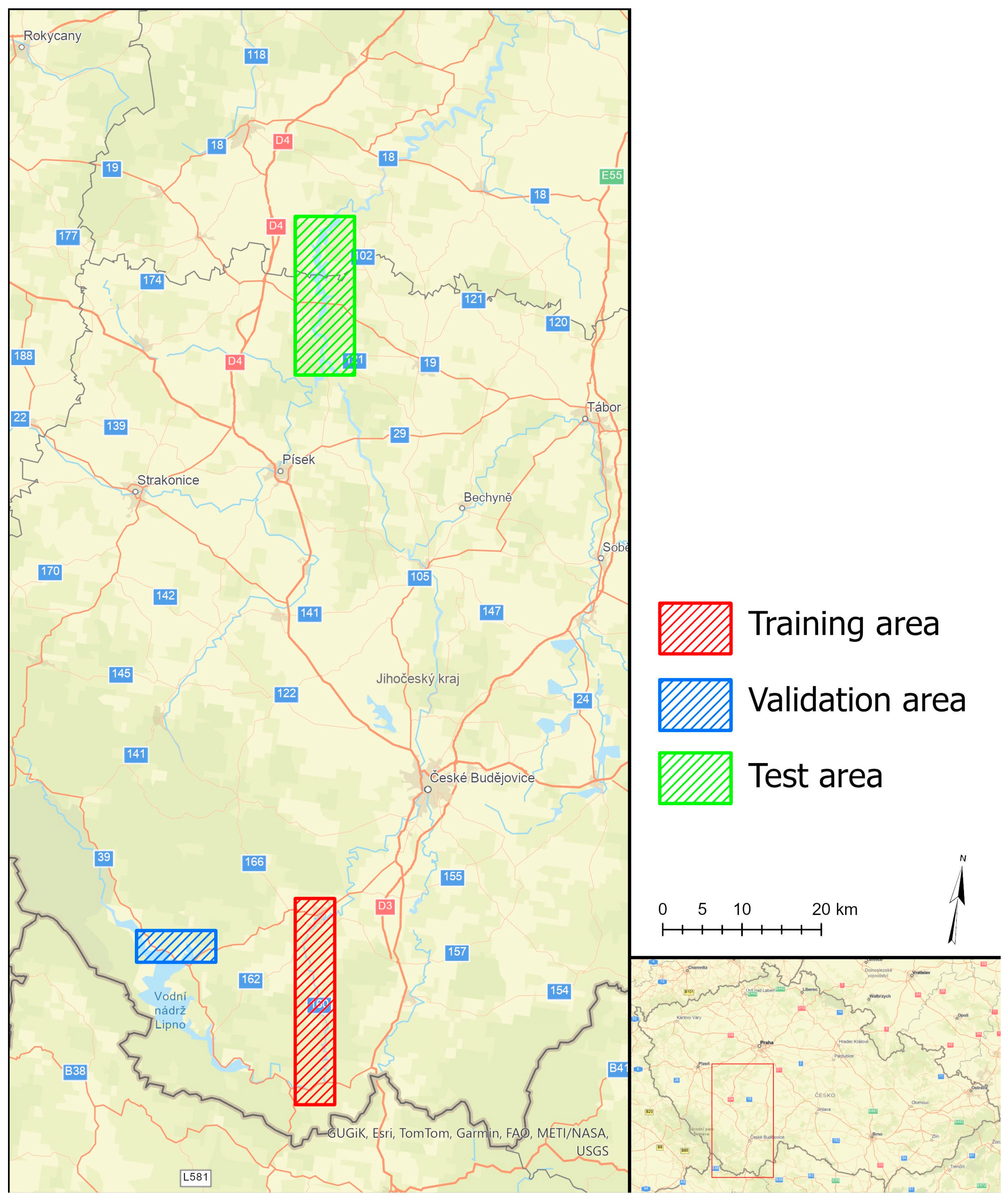
3.1. Area of Interest

The site of interest is the upper and middle course of the Vltava River historical valley. This valley was dammed in the second half of the 20th century, and the relief changed significantly. Some maps with elevation information describe this area before this change, one of them is the SMO-5 map. Regarding difficulties presented in this dataset, the individual SMO-5 map sheets differ significantly in many aspects. The individual map sheets were combined into a seamless map. Their processing and accuracy rating are given in [13]. Being created in different years by different teams of people, the map symbology shows noticeable changes, such as slightly different colors and contrast of scanned sheets. The sheets exhibit differing elevation intervals of contours, as sheets were produced either with 1-, 2-, 5-, 10-, or 20-m contour intervals. This often creates discontinuity between map sheets with contour cut-offs. Another source of topological errors comes from elevation annotations inserted in the contour lines with spaces between digits and lines. Similar interruptions are found in some dashed contour lines, marking intermediate elevations. Another difficulty arises from the occasionally steep terrain, where contour lines appear significantly dense, to the extent of nearly touching each other.

Leveraging previously vectorized map sheets, we use a selection of them to create train, validation, and test splits. Three different locations of the Vltava valley were used (Figure 1).

3.2. Extraction Methods

In his work, Chen proposed a two-stage method to obtain vectorized shapes, deep edge filtering (DEF), and closed shape extraction (CSE). To jointly optimize these two stages, a grid search for the best COCO-PQ metric was conducted, evaluating every DEF-trained epoch with all CSE parameters on the validation split with ground truth polygons. Many possibilities were tested; for DEF, tests were conducted with BDCN, HED, U-Net, ConnNet, different weight initializations, and data augmentations. Topology-aware losses were also considered. For CSE, thresholding was set as a baseline against Meyer watershed with various parameters to generate label maps, assigning a unique label to each pixel belonging to a distinct shape.

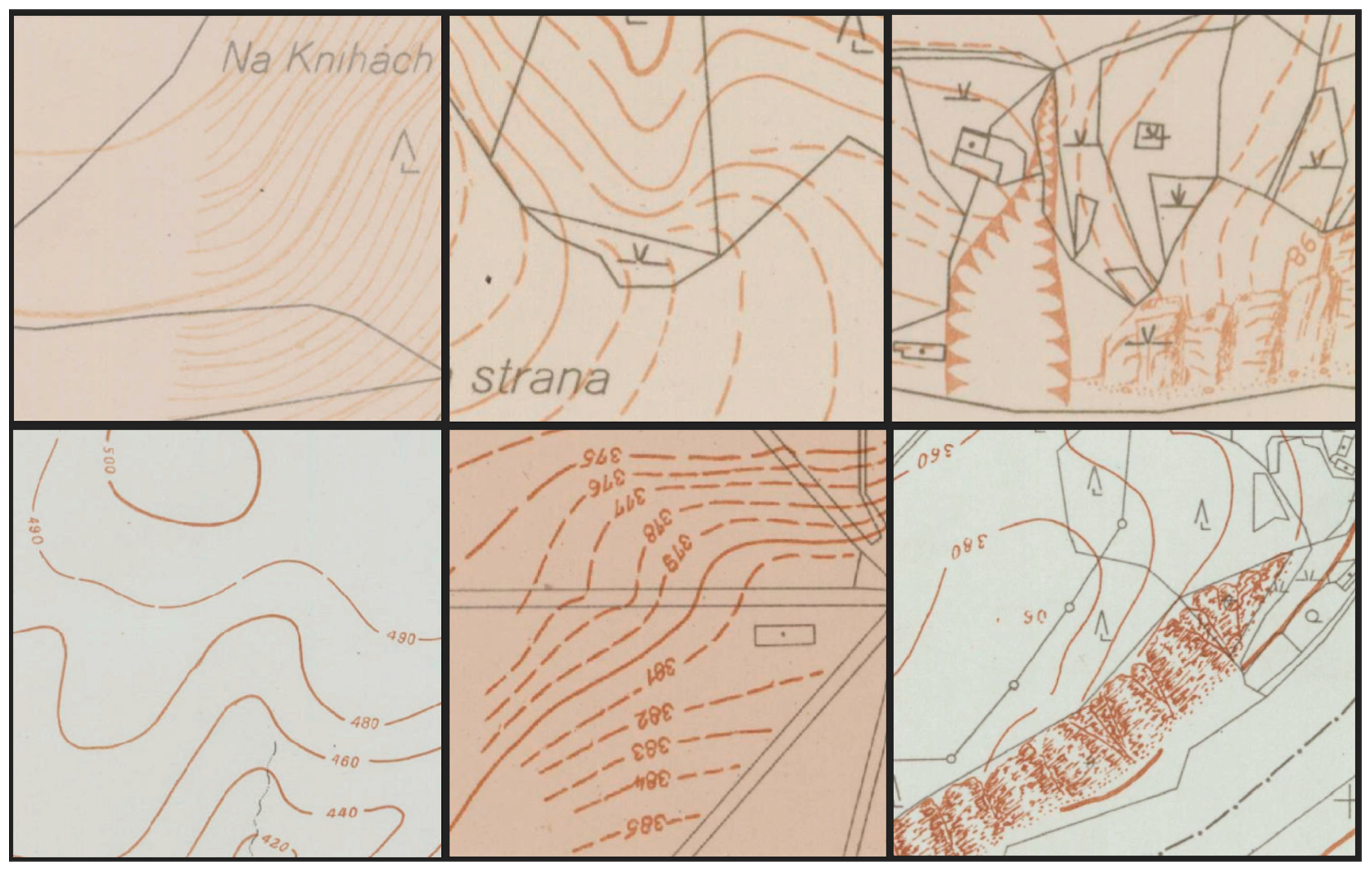
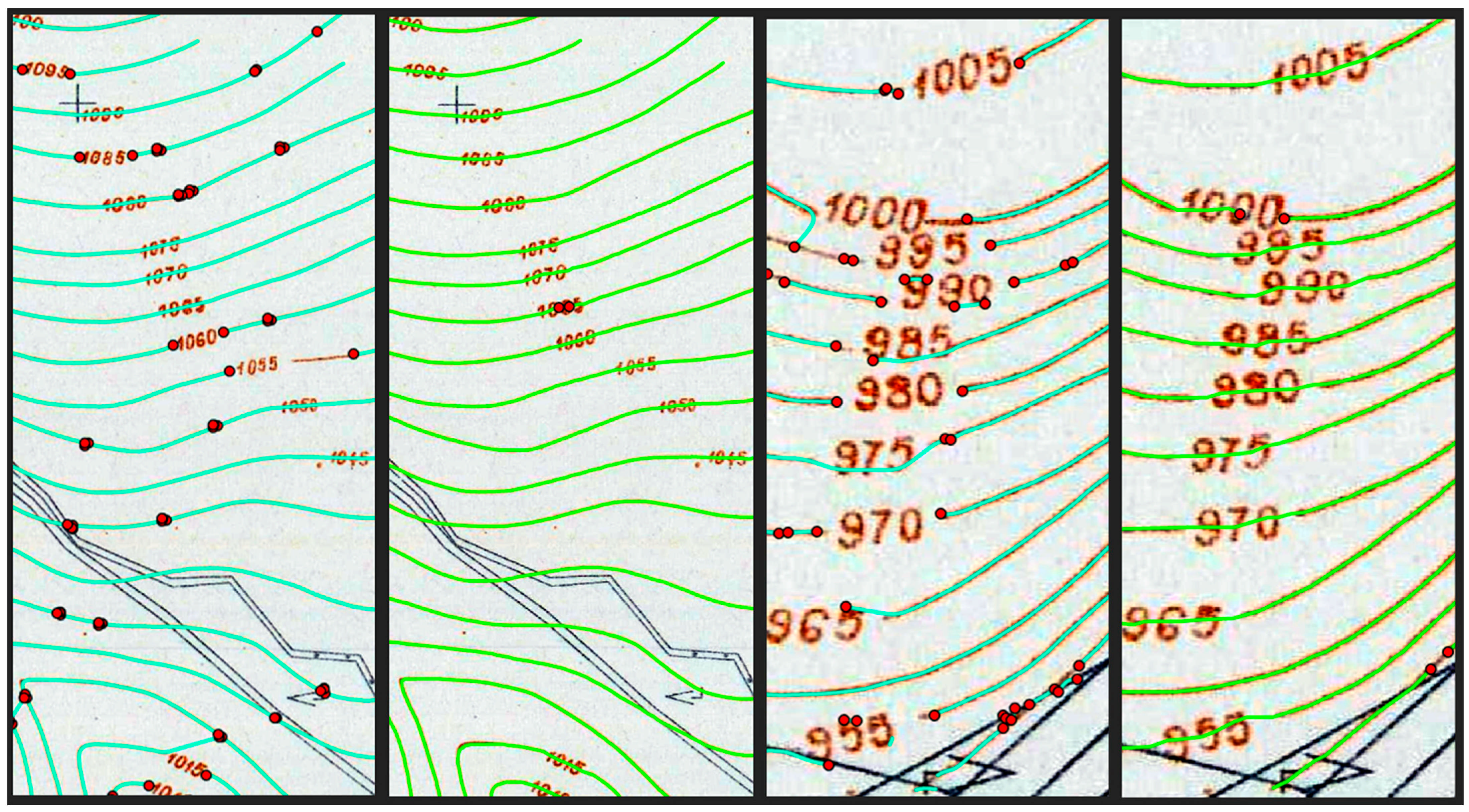
The above-described research dealt with cadaster maps, where enclosed polygons are advantageously conveniently extracted with Meyer watershed, which is able to recover even weakly signaled edges. For the task of elevation contour vectorization, there are a few differences. In theory, contours also always form closed shapes. The borders of scanned (and mosaicked) raster represent an artificial boundary that nonetheless can be included as a border of a closed shape. The real caveat lies in many intermediate contours and other interrupted contours, resulting in many dead ends (Figure 2). With this in mind, the CSE stage is irrelevant to us, and the watershed transform cannot be used.

Another difference lies in the thickness of line features. Whereas scanned Paris atlas maps consist of thin line features, SMO-5 map contours are of various thickness, generally notably wider. The ground truth label data for the Paris atlas were created by vectorizing and rasterizing the lines to one-pixel-wide raster lines. In training, these were additionally dilated by one pixel in each direction. While, in our case, the line elements are generally thicker and would perhaps benefit from a wider buffer zone, in many cases, the contours are quite densely placed. To avoid the merging of too wide segments in these situations, we also opt for only three-pixel-wide training masks.

For the DEF stage, Chen reported U-Net [40] with Kaiming initialization [41] as the best-performing network. For data augmentation, Chen recommends contrast stretching and thin plate spline (TPS) geometric modification. Chen also proposed and tested topology-aware losses, first training U-Net for 50 epochs and then continuing with loss functions such as Topoloss [42] or BALoss [43]. BALoss was tested to perform quite well on data without domain shift and can be thought of as an alternative to Meyer watershed, which we cannot use. Given the frequency of contour interruptions such as embedded elevation annotations and map sheet seams, this could help to preserve topological continuity.

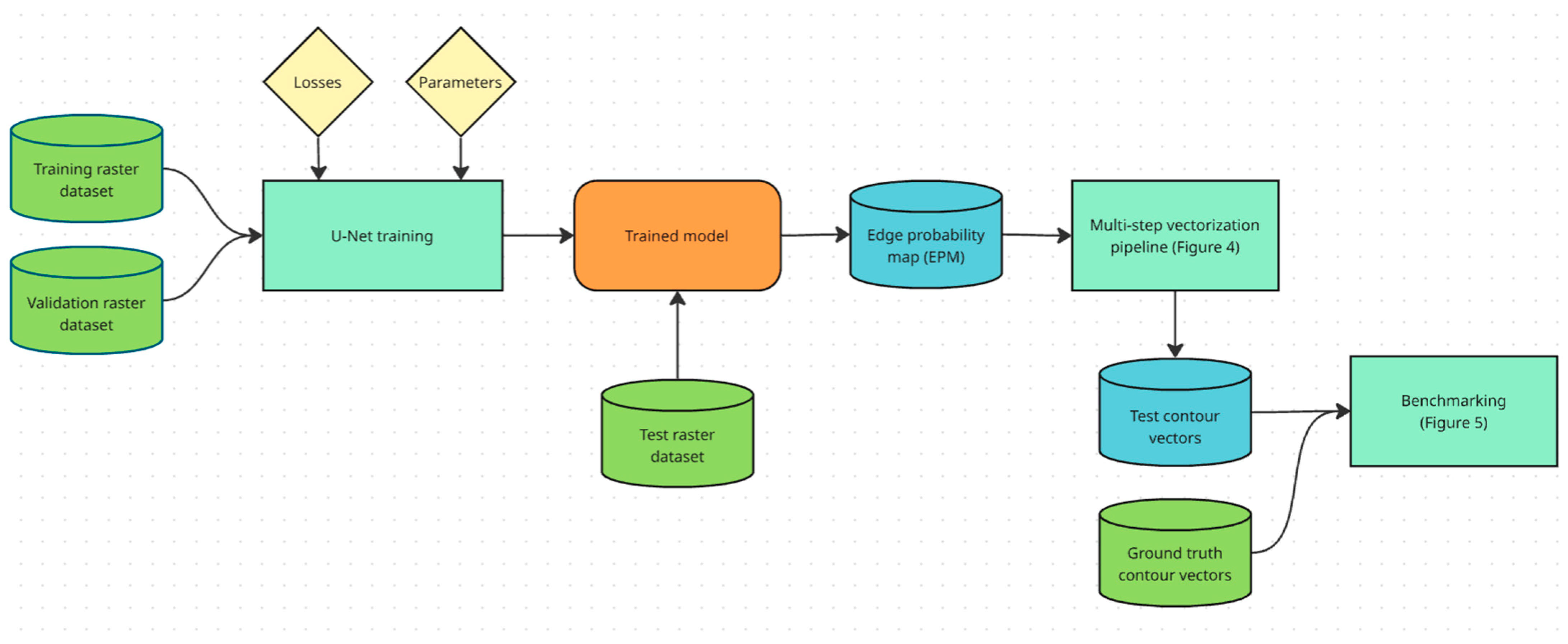
Our presented approach can be broken down into three stages. The first stage consists of training a deep neural network and creating an EPM raster by inferring the trained model on test data. The second stage comprises of multi-step vectorization pipeline, which vectorizes the EPM raster to final contours. Finally, the resulting vectors are compared to the ground truth vectors in benchmarking, allowing us to compare the results depending on various parameters. A simplified flowchart of the whole process is shown in Figure 3.

3.3. Training Experiments

The implemented smart data loader partitions the input raster into image chips of 500 × 500 pixels, with a padding half the size, resulting in 12,384 training chips and 5544 validation chips. Generally, we follow recommendations by Chen: all the experiments were conducted with a batch size of 4, a base learning rate of 1 × 10⁻⁴ with gradual reduction (plateau scheduler) to 1 × 10⁻⁵, and a weight decay of 2 × 10⁻⁴. As evident from

Table 1. Sites of interest used for training and testing the model.

	N. of Map Sheets	Area [km2]	Approx. Contour Area [km2]	Pct. of Contours [%]
Train	26	130	10.49	8.07
Validation	8	40	2.49	6.23
Test	27	135	3.67	2.72

, the classes are significantly imbalanced. This is handled in the weighted computation of the loss function. The loss function is set to binary cross-entropy, as the task is posed as a simple two-class segmentation. When training with additional topology loss, the additional loss is weighted and added to the cross-entropy loss, backpropagating both metrics simultaneously. For data augmentation, contrast stretching is used with random values between 0.8 and 1.25, as the map sheets differ quite noticeably in color signal. TPS geometric transformation proved to be quite slow in larger training (slowing down the process about eight times); therefore, we opted for affine transformation, which placed narrowly second in metrics, and did not introduce any significant bottleneck.

We train each model for 50 epochs. If a topology loss is used, it is trained atop the previous pretrained network for an additional 50 epochs. The model is then used for inference on the test split. The training was performed on an Nvidia GeForce 4070 Ti. One epoch took about twenty minutes to half an hour. Due to limited resources, we could not conduct more extensive testing; therefore, we limited the experiments to the most promising methods. These are U-Net with different configurations of data augmentation and topology loss (BALoss).

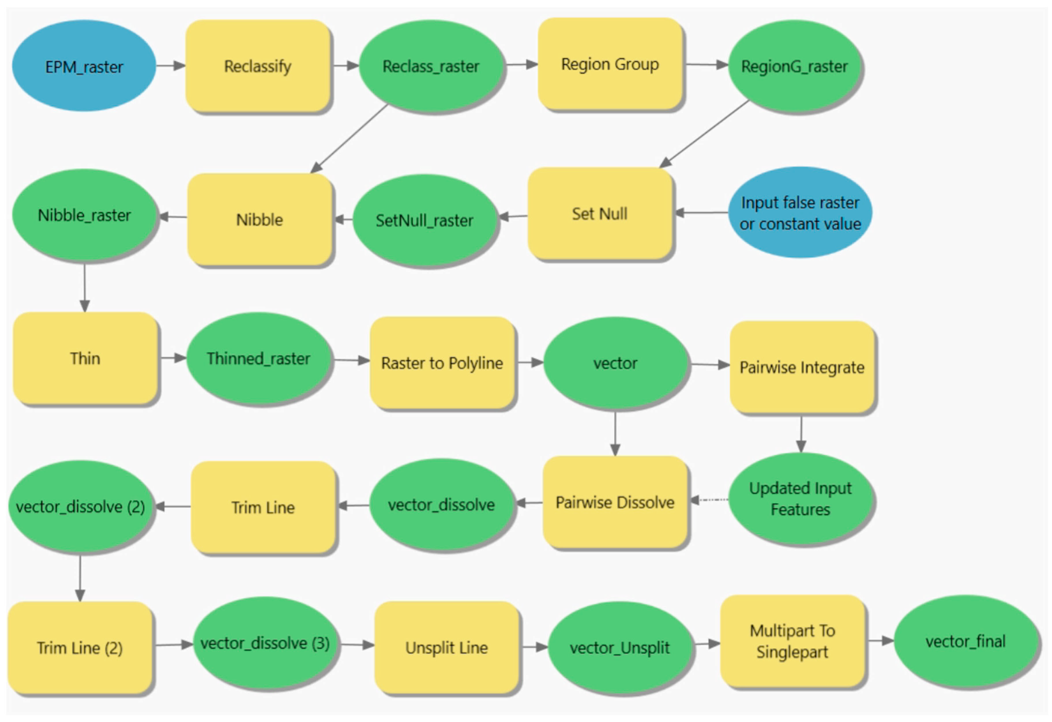
3.4. Raster to Vector Conversion and Postprocessing

To convert the EPM to a vectorized final output, the map is thresholded at 0.5. As discussed earlier, watershed segmentation cannot be used. The binary raster is then cleaned of small pixel clusters of size less than 400 pixels and thinned with a centerline. This thinned raster is then converted to a vector. To eliminate dangling lines originating from erroneous trisections, all dangles shorter than 25 m are trimmed. This does not remove circular dangles that sometimes result from thinning. To account for this, vertices closer than 0.85 m (two pixels) are integrated before the last step. Such an operation also slightly generalizes the contours. The overall pipeline is visually described in ArcGIS ModelBuilder in Figure 4. A step-by-step explanation is provided in Appendix A.

3.5. Benchmarking

To judge the trained models, we want to quantify the resulting topology errors, as topological consistency is the most important metric for our use case. The amount of topology errors is directly related to the amount of time and work a human operator would have to put in to correct the results. Pixel-level accuracy metrics are not crucial, as the resulting probability map is going to be thinned, and the contour area is generally segmented well in all experiments anyway. Positional precision is not of concern because the potential mistakes are too small to have any significant impact on any further result. The model can produce false positives/false negatives; however, these will be accounted for in topological errors. The COCO-PQ score cannot be used, as it is based on the intersection-over-union of closed shapes, which, as discussed earlier, are not the result. To quantify the topological errors, we simply count them on the test split. We do not consider the outer borders of the raster; therefore, a buffer zone of 25 m is used to eliminate border errors. Counted topological errors include contour interruptions or intersections with a different contour.

To compare the various models, we simply count the topological errors in the vector layer on the test set. A topological error in this scope is defined as follows:

(1)

Any kind of line intersection. Contours closely placed to each other can result in trisections, and any kind of intersection in this scenario is perceived as an error.

(2)

Any dangling line end, not located within a 15 m proximity to any ground truth dangling line end. Some intermediate contours do have loose ends even in the ground truth; therefore, we deduct them from testing so as not to penalize the evaluated models.

At this point, we have not annotated the vectorized contours with elevation; therefore, we do not assess whether only the contours of the same value are connected. These errors would likely result in another topological error elsewhere anyway, whether an intersection or a loose end. Many individual errors occur close to each other, due, for example, to an interrupting annotation creating multiple intersections and loose ends in one place. Thus, we sum up errors located within 10 m of each other and count them as one instance of an error, because they are likely correlated and would require the attention of a human operator to fix them. The final score is represented by the generalized sum of topological errors. Figure 5 shows the process implementation in ModelBuilder, further described in Appendix B.

4. Results

With the settings described earlier, four neural networks were trained:

(1)

Simple U-Net

(2)

U-Net with contrast and geometry augmentations

(3)

Augmented U-Net with BALoss, alpha 10

(4)

Augmented U-Net with BALoss, alpha 50

(5)

Augmented U-Net with BALoss, alpha 100

After training, these networks were applied to the test split consisting of two sheets with relatively dense contours. After the above-described processing, the errors were counted and are shown in

Table 2. Resulting topological errors under different training settings.

Model	Intersection Errors	Dangle Ends Errors	Combined Generalized Errors
U-Net	43	4474	2542
U-Net AUG	147	1396	797
U-Net AUG BALoss 10	163	1295	721
U-Net AUG BALoss 50	191	959	577
U-Net AUG BALoss 100	188	762	458

.

Augmentation clearly improves the vectorization precision significantly. The contrast stretching interval might arguably be too wide, resulting in some blurred predictions. Increasing the BALoss factor results in less conservative predictions, strengthening weak connections with potentially false positives. Stronger BALoss decreases dangling ends but increases unwanted intersections.

This is evident from a qualitative result in Figure 6. A more conservative original U-Net fails to recover some connections and results in dangles. With augmentation and BALoss factor increase, the predictions become more blurred and result in more intersections than dangles.

Subsequent vectorization succeeds in map sheets with sparse and well-defined contours, whereas it struggles with denser areas with gaps from annotations and dashed lines. Qualitative comparison in such areas favors the deep learning approach (Figure 7).

The U-Net inference time for the test split (30 map sheets) was about 15 min. The conversion of an EPM map to vector took about 7.5 min. While the first step is solely dependent on the input map resolution, the second step includes more operations and is also dependent on the number of contours. For increased scalability, the amount of available RAM can represent a constraint. In our case, the use of the numpy.memmap module allowed us to bypass this constraint by intermediately utilizing hard drive storage.

5. Discussion

Quantitative comparison on the same map with results obtained with thresholding vectorization [14] is unfortunately difficult. The ground truth data we were provided with were already manually finished in the postprocessing, with much of the manual editing already carried out in ArcScan without any provided intermediate results. The number of errors depends highly on the choice of thresholding interval, which is selected by trial-and-error for each map sheet. This results in uneven and irreproducible results. We are, therefore, left with only a crude qualitative comparison of some areas. The absolute number of errors in Table 2 can seem quite high. This is caused by, among other things, the discontinuity between map sheets, where all available methods will also suffer huge errors. The discontinuities are caused by the often-differing symbology rules, like the contour elevation interval, sudden change to a different type of line, or the frequent vertical shift. Many contours do not have any continuation beyond the seams, and even if they do, sometimes the adjacent contour is significantly shifted along the seam. Kratochvílová and Cajthaml [14] dealt with this problem by clipping the contours 10 m before the seams, annotating the vector data with elevation, and then connecting the lines across the seams based on the elevation attributes.

In the face of great spectral and figurative diversity, the results could be improved. Some map sheets demonstrate notably inferior results, specifically the ones with spectral properties extremely diverging from the average. This shows that the training dataset should be expanded to include chips from a plethora of sheets of different properties. This could also pave the way for a more general model, able to transfer the vectorization capabilities to a completely different map altogether. Current work can be expanded with training on different SMO-5 time series (1970, 1980) to ensure robustness across similar maps. This has not been performed in the scope of this article due to a lack of ground truth data and time and resource constraints.

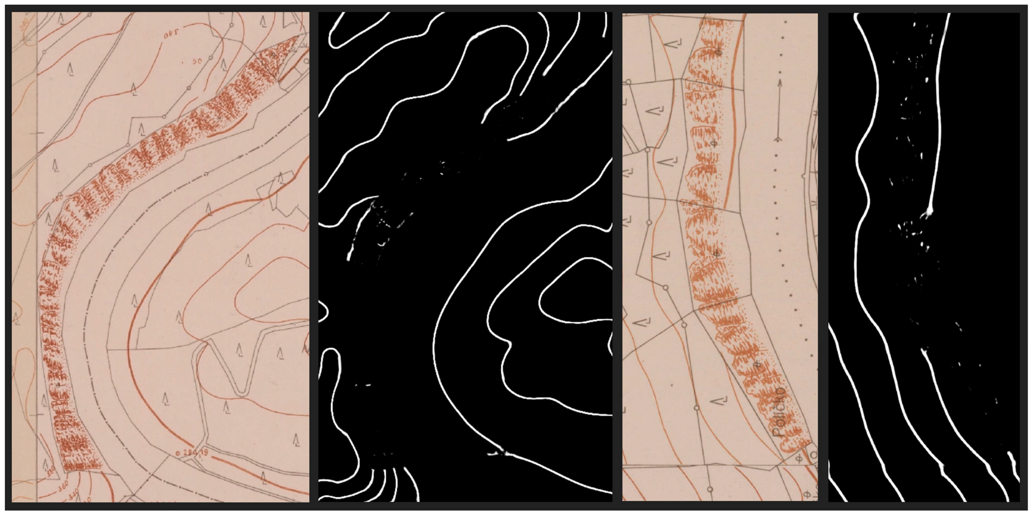
Steep rock sections marked with the same color as contours can be successfully segmented out, as demonstrated in Figure 8. Because these features are not abundantly present in the map, it is necessary to ensure sufficient representation of such cases in the training dataset.

While the vectorization postprocessing after inference presented in this article can be thought of as an alternative to the previous work [14], the resulting segmented map can also be used as an input to the ArcScan vectorization pipeline, which requires a binary raster. Obtaining this binary map is demanding because the thresholding values have to be set individually for each raster. EPMs resulting from U-Net inference can be used instead, as they handle the spectral and figurative diversity of different map sheets.

Another bulk of errors comes from interruptions by annotations. This is partly remedied by our approach, as demonstrated in Figure 7. Sometimes the connection is too weak, and the contour is interrupted. To strengthen contour probability connections, BALoss can be utilized, improving the error score, as evident in Table 2. To connect contours interrupted by a weak EPM signal, some automation could be achieved. Simple snap to closest is not reliable because the closest endpoint might belong to a contour of a different annotation. But a combination of distance and orientation of the two dangles could be utilized for more robust reconnections.

The naive EPM thresholding, where all pixels with a probability smaller than 0.5 are discarded, is not optimal due to the inflexibility of arbitrary parameter settings, discarding potential edges while preserving false dangles. Watershed transform could be used for the non-intermediate contours, which form closed shapes, which could improve the extraction results for a large percentage of total contours. These extracted contours could then be masked to extract the rest—intermediate contours with dead ends using generic arbitrary thresholding as currently used.

6. Conclusions

The neural network approach proved to be very useful. Thanks to a diverse set of training data representing differing symbology, the neural network is robust in different environments, and with augmentation, the model generalizes relatively well across different map sheets with distinct spectral properties. The valuable ability to bridge the gaps created by annotation, dashing, or other interruptions significantly improves the resulting topological consistency. Compared to previous research, the proposed approach reduces manual work in numerous aspects, such as manual thresholding for each map sheet, cleaning false positives with identical spectral properties (rocks, etc.), and, overall, fewer necessary topology corrections, especially in densely drawn places. Regardless of the chosen trained network, a large amount of manual work (tracing) is removed. Nonetheless, some manual corrections by human operators are still necessary. The main benefit of a neural network is the scalability, which allows us to process a lot of map sheets in one run. With the processing time of one sheet below one minute, the whole area of the Czech Republic, consisting of 16,301 SMO-5 map sheets, could be processed in a few hours. In the case of such an effort, it would be appropriate to collect ground truth data from various localities to ensure consistent results. A similar method can be applied to a variety of map vectorization tasks, where simple operations such as thresholding fail, and where the feature extraction requires wider context.

Future work will concentrate on reliable automatic detection and recognition of annotations. Such a task is tricky because of the ambiguity of rotated digits. The recognized elevations can then be directly inserted into the attribute of the vectorized contour. Inconsistencies in symbology (elevation interval) across map sheets would likely limit the process to first annotate map sheets separately and then merge the sheets. Also, because of prevalent annotation mistakes in original maps caused by human error, this process would have to be spatially validated with a system of checks to ensure sequential consistency of elevations.

References

- Vuorela, N.; Alho, P.; Kalliola, R. Systematic Assessment of Maps as Source Information in Landscape-change Research. Landsc. Res. 2002, 27, 141–166. [Google Scholar] [CrossRef]
- Picuno, P.; Cillis, G.; Statuto, D. Investigating the time evolution of a rural landscape: How historical maps may provide environmental information when processed using GIS. Ecol. Eng. 2019, 139, 105580. [Google Scholar] [CrossRef]
- Brůna, V.; Pacina, J.; Pacina, J.; Vajsová, E. Modelling the extinct landscape and settlement for preservation of cultural heritage. Città Stor. 2014, 9, 131–153. [Google Scholar]
- Sánchez-Pinto, I. Historical mapping vs. archaeology: Rethinking fort sancti spiritus (1527–1529). Hist. Archaeol. 2022, 57, 220–251. [Google Scholar] [CrossRef]
- Lilley, K.D. Mapping the medieval city: Plan analysis and urban history. Urban Hist. 2000, 27, 5–30. [Google Scholar] [CrossRef]
- Brůna, V.; Křováková, K. Interpretation of Stabile Cadastre maps for landscape ecology purposes. In Proceedings of the International Conference on Cartography and GIS, Borovets, Bulgaria, 20–23 September 2006. [Google Scholar]
- Vynikal, J.; Müllerová, J.; Pacina, J. Deep learning approaches for delineating wetlands on historical topographic maps. Trans. GIS 2024, 28, 1400–1411. [Google Scholar] [CrossRef]
- Pacina, J.; Novák, K.; Popelka, J. Georelief Transfiguration in Areas Affected by Open-cast Mining. Trans. GIS 2012, 16, 663–679. [Google Scholar] [CrossRef]
- Pacina, J.; Cajthaml, J.; Kratochvílová, D.; Popelka, J.; Dvořák, V.; Janata, T. Pre-Dam Valley Reconstruction based on archival spatial data sources: Methods, accuracy, and 3D printing possibilities. Trans. GIS 2021, 26, 385–420. [Google Scholar] [CrossRef]
- Talich, M.; Bohm, O.; Soukup, L. Classification of digitized old maps. In Advances and Trends in Geodesy, Cartography and Geoinformatics; CRC Press: Boca Raton, FL, USA, 2018; pp. 197–202. [Google Scholar] [CrossRef]
- Janovský, M. Pre-dam vltava river valley—A case study of 3D visualization of large-scale GIS datasets in Unreal Engine. ISPRS Int. J. Geo-Inf. 2024, 13, 344. [Google Scholar] [CrossRef]
- Dharmaraj, G. Algorithms for Automatic Vectorization of Scanned Maps. Master’s Thesis, Department of Geomatics Engineering, The University of Calgary, Calgary, AB, Canada, 2005. [Google Scholar]
- Schlegel, I. A holistic workflow for semi-automated object extraction from large-scale historical maps. KN-J. Cartogr. Geogr. Inf. 2023, 73, 3–18. [Google Scholar] [CrossRef]
- Kratochvílová, D.; Cajthaml, J. Using the automatic vectorisation method in generating the vector altimetry of the historical Vltava River Valley. Acta Polytech. 2020, 60, 303–312. [Google Scholar] [CrossRef]
- Talich, M.; Antoš, F.; Böhm, O. Automatic processing of the first release of derived state maps series for web publication. In Proceedings of the 25th International Cartographic Conference (ICC2011) and the 15th General Assembly of the International Cartographic Association, Paris, France, 3–8 July 2011. [Google Scholar]
- Iosifescu, I.; Tsorlini, A.; Hurni, L. Towards a comprehensive methodology for automatic vectorization of raster historical maps. e-Perimetron 2016, 11, 57–76. [Google Scholar]
- Auffret, A.G.; Kimberley, A.; Plue, J.; Skånes, H.; Jakobsson, S.; Waldén, E.; Wennbom, M.; Wood, H.; Bullock, J.M.; Cousins, S.A.; et al. HistMapR: Rapid Digitization of historical land-use maps in R. Methods Ecol. Evol. 2017, 8, 1453–1457. [Google Scholar] [CrossRef]
- Oka, S.; Garg, A.; Varghese, K. Vectorization of contour lines from scanned topographic maps. Autom. Constr. 2012, 22, 192–202. [Google Scholar] [CrossRef]
- LeCun, Y.; Bengio, Y.; Hinton, G. Deep learning. Nature 2015, 521, 436–444. [Google Scholar] [CrossRef]
- LeCun, Y.; Bengio, Y. Convolutional networks for images, speech, and time series. In The Handbook of Brain Theory and Neural Networks; MIT Press: Cambridge, MA, USA, 1995; pp. 255–258. [Google Scholar]
- Minaee, S.; Boykov, Y.Y.; Porikli, F.; Plaza, A.J.; Kehtarnavaz, N.; Terzopoulos, D. Image segmentation using Deep Learning: A Survey. IEEE Trans. Pattern Anal. Mach. Intell. 2021, 44, 3523–3542. [Google Scholar] [CrossRef]
- Zhu, X.X.; Tuia, D.; Mou, L.; Xia, G.-S.; Zhang, L.; Xu, F.; Fraundorfer, F. Deep learning in remote sensing: A comprehensive review and list of resources. IEEE Geosci. Remote Sens. Mag. 2017, 5, 8–36. [Google Scholar] [CrossRef]
- Pesek, O.; Krisztian, L.; Landa, M.; Metz, M.; Neteler, M. Convolutional neural networks for road surface classification on aerial imagery. PeerJ Comput. Sci. 2024, 10, e2571. [Google Scholar] [CrossRef]
- Osco, L.P.; Marcato Junior, J.; Marques Ramos, A.P.; de Castro Jorge, L.A.; Fatholahi, S.N.; de Andrade Silva, J.; Matsubara, E.T.; Pistori, H.; Gonçalves, W.N.; Li, J. A review on deep learning in UAV Remote Sensing. Int. J. Appl. Earth Obs. Geoinf. 2021, 102, 102456. [Google Scholar] [CrossRef]
- Zahradník, D.; Roučka, F.; Karlovská, L. Flat roof classification and leaks detections by Deep Learning. Staveb. Obz.-Civ. Eng. J. 2024, 32, 564–576. [Google Scholar] [CrossRef]
- He, Y.; Yu, H.; Liu, X.; Yang, Z.; Sun, W.; Anwar, S.; Mian, A. Deep Learning based 3D segmentation in Computer Vision: A survey. Inf. Fusion 2025, 115, 102722. [Google Scholar] [CrossRef]
- Jiao, C.; Heitzler, M.; Hurni, L. Extracting wetlands from Swiss historical maps with Convolutional neural Networks. Automatic Vectorisation of Historical Maps. In Proceedings of the International workshop organized by the ICA Commission on Cartographic Heritage, Digital, Budapest, Hungary, 13 March 2020. [Google Scholar] [CrossRef]
- Maxwell, A.E.; Bester, M.S.; Guillen, L.A.; Ramezan, C.A.; Carpinello, D.J.; Fan, Y.; Hartley, F.M.; Maynard, S.M.; Pyron, J.L. Semantic segmentation deep learning for extracting surface mine extents from historic topographic maps. Remote Sens. 2020, 12, 4145. [Google Scholar] [CrossRef]
- Uhl, J.; Leyk, S.; Chiang, Y.-Y.; Duan, W.; Knoblock, C. Extracting human settlement footprint from Historical Topographic map series using context-based machine learning. In Proceedings of the 8th International Conference of Pattern Recognition Systems (ICPRS 2017), Madrid, Spain, 11–13 July 2017. [Google Scholar] [CrossRef]
- Garcia-Molsosa, A.; Orengo, H.A.; Lawrence, D.; Philip, G.; Hopper, K.; Petrie, C.A. Potential of deep learning segmentation for the extraction of archaeological features from historical map series. Archaeol. Prospect. 2021, 28, 187–199. [Google Scholar] [CrossRef]
- Petitpierre, R.; Kaplan, F.; di Lenardo, I. Generic semantic segmentation of historical maps. In Proceedings of the Computational Humanities Research Conference, Virtual, 17–19 November 2021; pp. 228–248. [Google Scholar]
- Ekim, B.; Sertel, E.; Kabadayı, M.E. Automatic road extraction from historical maps using Deep Learning Techniques: A regional case study of Turkey in a German World War II map. ISPRS Int. J. Geo-Inf. 2021, 10, 492. [Google Scholar] [CrossRef]
- Can, Y.S.; Gerrits, P.J.; Kabadayi, M.E. Automatic detection of road types from the third military mapping survey of Austria-Hungary historical map series with deep convolutional Neural Networks. IEEE Access 2021, 9, 62847–62856. [Google Scholar] [CrossRef]
- Uhl, J.H.; Leyk, S.; Chiang, Y.-Y.; Knoblock, C.A. Towards the automated large-scale reconstruction of past road networks from historical maps. Comput. Environ. Urban Syst. 2022, 94, 101794. [Google Scholar] [CrossRef]
- Khotanzad, A.; Zink, E. Contour line and geographic feature extraction from USGS color topographical paper maps. IEEE Trans. Pattern Anal. Mach. Intell. 2003, 25, 18–31. [Google Scholar] [CrossRef]
- Zhao, Y.; Wang, G.; Yang, J.; Li, T.; Li, Z. Au3-Gan: A Method for extracting roads from historical maps based on an attention generative adversarial network. J. Geovis. Spat. Anal. 2024, 8, 26. [Google Scholar] [CrossRef]
- Chen, Y.; Carlinet, E.; Chazalon, J.; Mallet, C.; Duménieu, B.; Perret, J. Vectorization of historical maps using deep edge filtering and closed shape extraction. Lect. Notes Comput. Sci. 2021, 510–525. [Google Scholar] [CrossRef]
- Chen, Y.; Carlinet, E.; Chazalon, J.; Mallet, C.; Duménieu, B.; Perret, J. Modern Vectorization and Alignment of Historical Maps: An Application to Paris Atlas (1789–1950). Ph.D. Thesis, IGN (Institut National de l’Information Géographique et Forestière), Saint-Mandé, France, 2023. [Google Scholar]
- Chen, Y.; Chazalon, J.; Carlinet, E.; Ngoc, M.Ô.V.; Mallet, C.; Perret, J. Automatic vectorization of historical maps: A benchmark. PLoS ONE 2024, 19, e0298217. [Google Scholar] [CrossRef]
- Ronneberger, O.; Fischer, P.; Brox, T. U-Net: Convolutional Networks for Biomedical Image Segmentation. In Proceedings of the Medical Image Computing and Computer-Assisted Intervention—MICCAI 2015, Munich, Germany, 5–9 October 2015; Lecture Notes in Computer Science. pp. 234–241. [Google Scholar] [CrossRef]
- He, K.; Zhang, X.; Ren, S.; Sun, J. Delving deep into rectifiers: Surpassing human-level performance on ImageNet Classification. In Proceedings of the 2015 IEEE International Conference on Computer Vision (ICCV), Santiago, Chile, 7–13 December 2015. [Google Scholar] [CrossRef]
- Hu, X.; Li, F.; Samaras, D.; Chen, C. Topology-preserving deep image segmentation. In Advances in Neural Information Processing Systems; MIT Press: Cambridge, MA, USA, 2019; p. 32. [Google Scholar]
- Ngoc, M.; Chen, Y.; Boutry, N.; Chazalon, J.; Carlinet, E.; Fabrizio, J.; Mallet, C.; Géraud, T. Introducing the Boundary-Aware loss for deep image segmentation. In Proceedings of the British Machine Vision Conference (BMVC), Virtual, 23–25 November 2021; Volume 17. [Google Scholar]